
Coordination Relationship of Carbon Emissions and Air Pollutants under Governance Measures in a Typical Industrial City in China

 ,
,
Abstract
:1. Introduction
2. Methodology
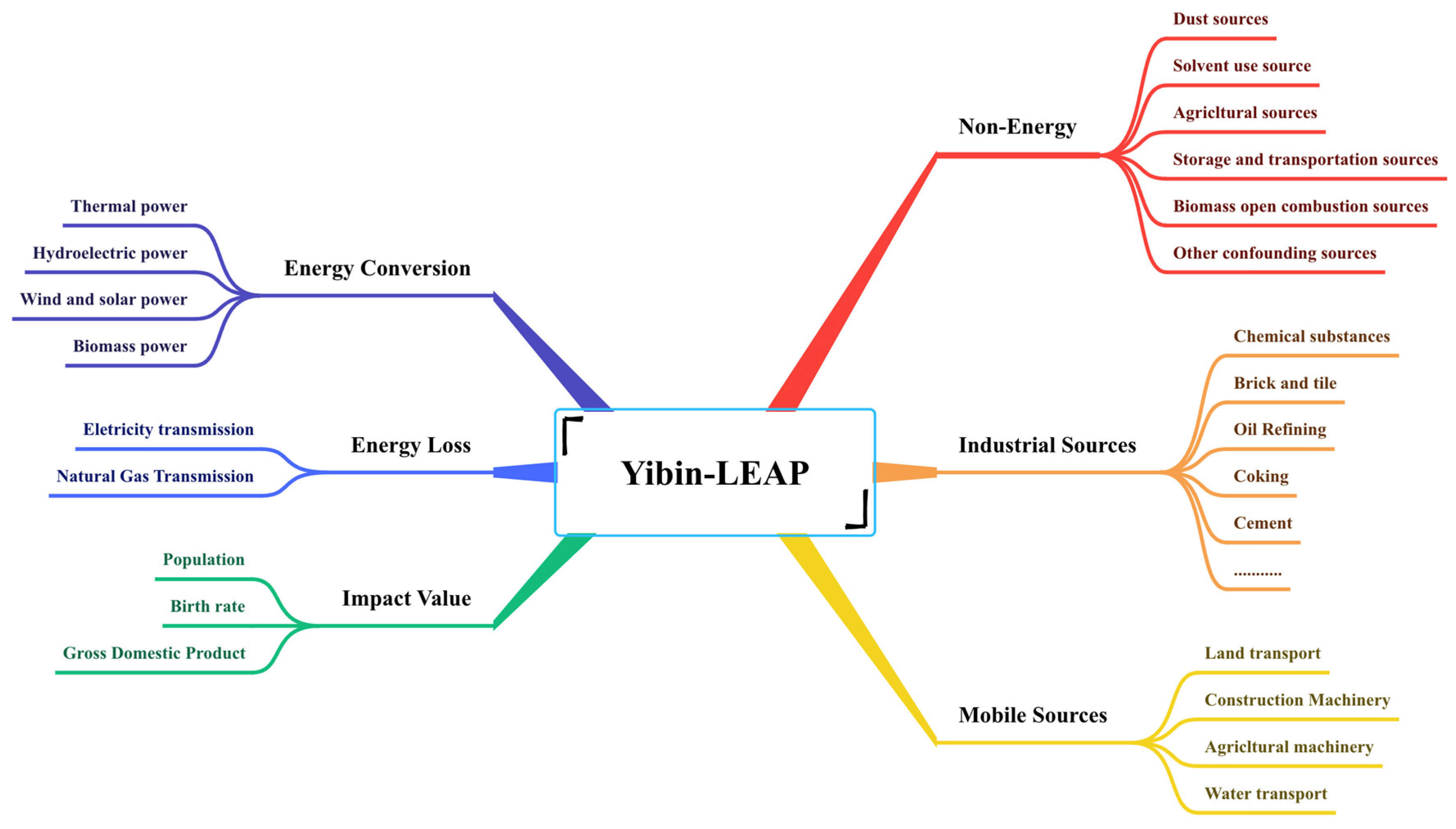
2.1. Carbon Emission Model
2.2. Air Quality Model
2.3. Model Scenarios and Settings
2.4. Air Quality Comprehensive Index
3. Results and Discussion
3.1. Model Verification
3.2. Analysis of Carbon Peak Targets
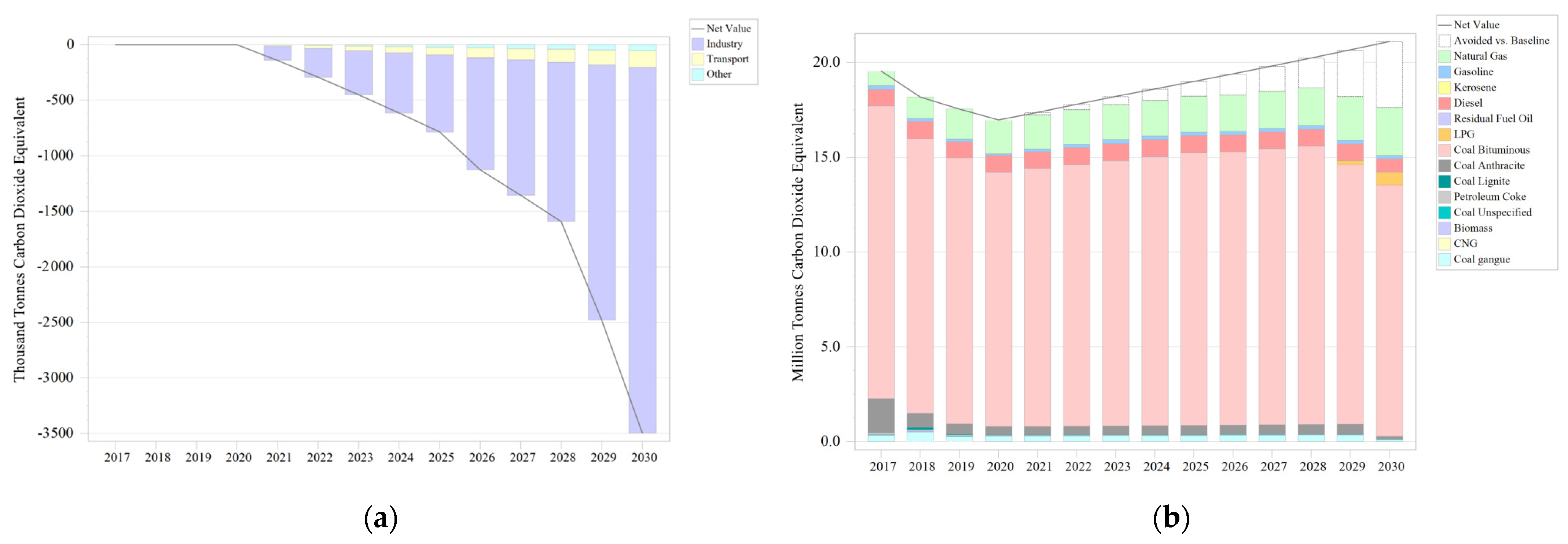
3.3. Carbon Peak under the Integration Scenario
3.4. Pollutant Reduction Ratio under Carbon Peak
3.5. Air Quality Improvement
3.6. Analysis of Coordination Relationship
4. Conclusions
Author Contributions
Funding
Institutional Review Board Statement
Informed Consent Statement
Data Availability Statement
Acknowledgments
Conflicts of Interest
References
- Dong, Z.; Xia, C.; Fang, K.; Zhang, W. Effect of the carbon emissions trading policy on the co-benefits of carbon emissions reduction and air pollution control. Energy Policy 2022, 165, 112998. [Google Scholar] [CrossRef]
- Zeebe, R.E. History of seawater carbonate chemistry, atmospheric CO2, and ocean acidification. Annu. Rev. Earth Planet. Sci. 2012, 40, 141–165. [Google Scholar] [CrossRef]
- Duman, Z.; Mao, X.; Cai, B.; Zhang, Q.; Chen, Y.; Gao, Y.; Guo, Z. Exploring the spatiotemporal pattern evolution of carbon emissions and air pollution in Chinese cities. J. Environ. Manag. 2023, 345, 118870. [Google Scholar] [CrossRef] [PubMed]
- Canadell, J.G.; Le Quéré, C.; Raupach, M.R.; Field, C.B.; Buitenhuis, E.T.; Ciais, P.; Conway, T.J.; Gillett, N.P.; Houghton, R.; Marland, G. Contributions to accelerating atmospheric CO2 growth from economic activity, carbon intensity, and efficiency of natural sinks. Proc. Natl. Acad. Sci. USA 2007, 104, 18866–18870. [Google Scholar] [CrossRef] [PubMed]
- Zeng, Q.H.; He, L.Y. Study on the synergistic effect of air pollution prevention and carbon emission reduction in the context of "dual carbon": Evidence from China’s transport sector. Energy Policy 2023, 173, 113370. [Google Scholar] [CrossRef]
- Cao, G.; Zhang, X.; Wang, Y.; Zheng, F. Estimation of emissions from field burning of crop straw in China. Chin. Sci. Bull. 2008, 53, 784–790. [Google Scholar] [CrossRef]
- Zhu, J.; Wu, S.; Xu, J. Synergy between pollution control and carbon reduction: China’s evidence. Energy Econ. 2023, 119, 106541. [Google Scholar] [CrossRef]
- Hossain, M.F. Extreme level of CO2 accumulation into the atmosphere due to the unequal global carbon emission and sequestration. Water Air Soil Pollut. 2022, 233, 105. [Google Scholar] [CrossRef]
- Rehman, A.; Ulucak, R.; Murshed, M.; Ma, H.; Işık, C. Carbonization and atmospheric pollution in China: The asymmetric impacts of forests, livestock production, and economic progress on CO2 emissions. J. Environ. Manag. 2021, 294, 113059. [Google Scholar] [CrossRef]
- Zhao, Y.; Duan, X.; Yu, M. Calculating carbon emissions and selecting carbon peak scheme for infrastructure construction in Liaoning Province, China. J. Clean. Prod. 2023, 420, 138396. [Google Scholar] [CrossRef]
- People’s Government of Yibin City. 2022 Yibin Socio-Economic Bulletin. 2022. Available online: http://www.yibin.gov.cn/xxgk/zdlyxxgk/tjxx/index.html (accessed on 8 December 2023).
- Sichuan Bureau of Statistics. 2022 Sichuan Provincial Statistical Yearbook. 2022. Available online: http://tjj.sc.gov.cn/scstjj/c105855/nj.shtml (accessed on 8 December 2023).
- Shu, Z.; Zhao, T.; Liu, Y.; Zhang, L.; Ma, X.; Kuang, X.; Li, Y.; Huo, Z.; Ding, Q.; Sun, X. Impact of deep basin terrain on PM2.5 distribution and its seasonality over the Sichuan Basin, Southwest China. Environ. Pollut. 2022, 300, 118944. [Google Scholar] [CrossRef] [PubMed]
- Kou, Y.; Xian, D.; Liu, Y.; Chen, J.; Wang, C.; Cheng, B.; Guo, W.; Li, Y.; Tang, L. Factors affecting urban climate at different times of the day in China: A case study in Yibin, a riverside mountain city. Nat. Based Solut. 2022, 2, 100043. [Google Scholar] [CrossRef]
- Shu, Z.; Liu, Y.; Zhao, T.; Xia, J.; Wang, C.; Cao, L.; Wang, H.; Zhang, L.; Zheng, Y.; Shen, L. Elevated 3D structures of PM2.5 and impact of complex terrain-forcing circulations on heavy haze pollution over Sichuan Basin, China. Atmos. Chem. Phys. 2021, 21, 9253–9268. [Google Scholar] [CrossRef]
- Department of Ecology and Environment of Sichuan Province. Air quality in Sichuan Province in 2021. 2022. Available online: https://sthjt.sc.gov.cn/ (accessed on 8 December 2023).
- Shabbir Alam, M.; Duraisamy, P.; Bakkar Siddik, A.; Murshed, M.; Mahmood, H.; Palanisamy, M.; Kirikkaleli, D. The impacts of globalization, renewable energy, and agriculture on CO2 emissions in India: Contextual evidence using a novel composite carbon emission-related atmospheric quality index. Gondwana Res. 2023, 119, 384–401. [Google Scholar] [CrossRef]
- Wang, H.; Gu, K.; Sun, H.; Xiao, H. Reconfirmation of the symbiosis on carbon emissions and air pollution: A spatial spillover perspective. Sci. Total Environ. 2023, 858, 159906. [Google Scholar] [CrossRef] [PubMed]
- Tawalbeh, L.A.; Delgado, J.; Solis, S.; Juarez, T.; Tietjen, J.D.; Muheidat, F. Energy Consumption and Carbon Emissions Data Analysis: Case Study and Future Predictions. Procedia Comput. Sci. 2023, 220, 616–623. [Google Scholar] [CrossRef]
- He, M.; Wang, X.; Han, L. Emission Inventory and Characteristics of Anthropogenic Air Pollution Sources Based on Second Pollution Source Census Data in Sichuan Province. Acta Sci. Circumstantiae 2013, 41, 3127–3137. [Google Scholar] [CrossRef]
- Yang, X.; Wu, Q.; Zhao, R.; Cheng, H.; He, H.; Ma, Q.; Wang, L.; Luo, H. New method for evaluating winter air quality: PM2.5 assessment using Community Multi-Scale Air Quality Modeling (CMAQ) in Xi’an. Atmos. Environ. 2019, 211, 18–28. [Google Scholar] [CrossRef]
- Bai, C.; Chen, Z.; Wang, D. Transportation carbon emission reduction potential and mitigation strategy in China. Sci. Total Environ. 2023, 873, 162074. [Google Scholar] [CrossRef]
- Zhang, C.; Luo, H. Research on carbon emission peak prediction and path of China’s public buildings: Scenario analysis based on LEAP model. Energy Build. 2023, 289, 113053. [Google Scholar] [CrossRef]
- El-Sayed, A.H.A.; Khalil, A.; Yehia, M. Modeling alternative scenarios for Egypt 2050 energy mix based on LEAP analysis. Energy 2023, 266, 126615. [Google Scholar] [CrossRef]
- Huang, Y.; Wang, Y.; Peng, J.; Li, F.; Zhu, L.; Zhao, H.; Shi, R. Can China achieve its 2030 and 2060 CO2 commitments? Scenario analysis based on the integration of LEAP model with LMDI decomposition. Sci. Total Environ. 2023, 888, 164151. [Google Scholar] [CrossRef] [PubMed]
- De Angelis, E.; Turrini, E.; Carnevale, C.; Volta, M. Vehicle fleet electrification: Impacts on energy demand, air quality and GHG emissions. An integrated assessment approach. IFAC-PapersOnLine 2020, 53, 16581–16586. [Google Scholar] [CrossRef]
- Dong, H.; Dai, H.; Geng, Y.; Fujita, T.; Liu, Z.; Xie, Y.; Wu, R.; Fujii, M.; Masui, T.; Tang, L. Exploring impact of carbon tax on China’s CO2 reductions and provincial disparities. Renew. Sustain. Energy Rev. 2017, 77, 596–603. [Google Scholar] [CrossRef]
- Eldowma, I.A.; Zhang, G.; Su, B. The nexus between electricity consumption, carbon dioxide emissions, and economic growth in Sudan (1971–2019). Energy Policy 2023, 176, 113510. [Google Scholar] [CrossRef]
- Krapivin, V.F.; Varotsos, C.A.; Soldatov, V.Y. Simulation results from a coupled model of carbon dioxide and methane global cycles. Ecol. Model. 2017, 359, 69–79. [Google Scholar] [CrossRef]
- Varotsos, C.; Mazei, Y.; Efstathiou, M. Paleoecological and recent data show a steady temporal evolution of carbon dioxide and temperature. Atmos. Pollut. Res. 2020, 11, 714–722. [Google Scholar] [CrossRef]
- Wu, H.; Yang, Y.; Li, W. Analysis of spatiotemporal evolution characteristics and peak forecast of provincial carbon emissions under the dual carbon goal: Considering nine provinces in the Yellow River basin of China as an example. Atmos. Pollut. Res. 2023, 14, 101828. [Google Scholar] [CrossRef]
- IPCC. 2019 Refinement to the 2006 IPCC Guidelines for National Greenhouse Gas Inventories. 2019. Available online: https://www.ipcc.ch/report/2019-refinement-to-the-2006-ipcc-guidelines-for-national-greenhouse-gas-inventories/ (accessed on 17 May 2023).
- Wang, Z.; Lv, J.; Tan, Y.; Guo, M.; Gu, Y.; Xu, S.; Zhou, Y. Temporospatial variations and Spearman correlation analysis of ozone concentrations to nitrogen dioxide, sulfur dioxide, particulate matters and carbon monoxide in ambient air, China. Atmos. Pollut. Res. 2019, 10, 1203–1210. [Google Scholar] [CrossRef]
- Houyoux, M.R.; Vukovich, J.M.; Coats, C.J.; Wheeler, N.J.M.; Kasibhatla, P.S. Emission inventory development and processing for the Seasonal Model for Regional Air Quality (SMRAQ) project. J. Geophys. Res. Atmos. 2000, 105, 9079–9090. [Google Scholar] [CrossRef]
- Williams, M.L. UK air quality in 2050—Synergies with climate change policies. Environ. Sci. Policy 2007, 10, 169–175. [Google Scholar] [CrossRef]
- Yu, Y.; Sokhi, R.S.; Kitwiroon, N.; Middleton, D.R.; Fisher, B. Performance characteristics of MM5–SMOKE–CMAQ for a summer photochemical episode in southeast England, United Kingdom. Atmos. Environ. 2008, 42, 4870–4883. [Google Scholar] [CrossRef]
- Yibin Municipal Bureau of Statistics. Yibin Statistics Yearbook; China Statistics Press: Beijing, China, 2022. Available online: http://tjj.yibin.gov.cn/sjfb/tjnj/ (accessed on 20 May 2023).
- Wang, S.; Pan, B.; Zhang, J.; Xie, S.; Gong, Z.; Li, L. Comparison study on the calculation methods of ambient air quality comprehensive index. Environ. Monit. China 2014, 30, 46–52. [Google Scholar] [CrossRef]
- MME (Ministry of Ecology and Environment of People’s Republic of China). Technical Regulation for Ambient Air Quality Assessment (on Trial). 2013. Available online: https://www.mee.gov.cn/ywgz/fgbz/bz/bzwb/jcffbz/201309/t20130925_260809.htm (accessed on 20 May 2023).
- Jiang, Z.; Gao, Y.; Cao, H.; Diao, W.; Yao, X.; Yuan, C.; Fan, Y.; Chen, Y. Characteristics of ambient air quality and its air quality index (AQI) model in Shanghai, China. Sci. Total Environ. 2023, 896, 165284. [Google Scholar] [CrossRef] [PubMed]
- Sirikalaya, S.; Chakrapan, C. The Study of Dispersion of Air Pollution in Ambient Environment-Case Study Map-Ta Industrial Estate. J. Aerosol Sci. 2004, 35, S1245–S1246. [Google Scholar] [CrossRef]
- Carnevale, C.; De Angelis, E.; Finzi, G.; Pederzoli, A.; Turrini, E.; Volta, M. A non linear model approach to define priority for air quality control. IFAC-PapersOnLine 2018, 51, 210–215. [Google Scholar] [CrossRef]
- Huang, L.; Zhu, Y.; Wang, Q.; Zhu, A.; Liu, Z.; Wang, Y.; Allen, D.T.; Li, L. Assessment of the effects of straw burning bans in China: Emissions, air quality, and health impacts. Sci. Total Environ. 2021, 789, 147935. [Google Scholar] [CrossRef]
- Li, L.; Zhu, S.; An, J.; Zhou, M.; Wang, H.; Yan, R.; Qiao, L.; Tian, X.; Shen, L.; Huang, L. Evaluation of the effect of regional joint-control measures on changing photochemical transformation: A comprehensive study of the optimization scenario analysis. Atmos. Chem. Phys. 2019, 19, 9037–9060. [Google Scholar] [CrossRef]
- Zhou, X.; Xu, Z.; Yan, J.; Liang, L.; Pan, D. Carbon emission peak forecasting and scenario analysis: A case study of educational buildings in Shanghai city. J. Build. Eng. 2023, 76, 107256. [Google Scholar] [CrossRef]
- Irina, D.; Luca, D.M.; James, W. PM2.5 analog forecast and Kalman filter post-processing for the Community Multiscale Air Quality (CMAQ) model. Atmos. Environ. 2015, 119, 431–442. [Google Scholar] [CrossRef]
- Chen, J.; Feng, X.; Zhu, Y.; Huang, L.; He, M.; Li, Y.; Yaluk, E.; Han, L.; Wang, J.; Qiao, Y.; et al. Assessment of the Effect of the Three-Year Action Plan to Fight Air Pollution on Air Quality and Associated Health Benefits in Sichuan Basin, China. Sustainability 2021, 13, 10968. [Google Scholar] [CrossRef]
- Kleeman, M.J.; Zapata, C.; Stilley, J.; Hixson, M. PM2.5 co-benefits of climate change legislation part 2: California governor’s executive order S-3-05 applied to the transportation sector. Clim. Change 2012, 117, 399–414. [Google Scholar] [CrossRef]
- Xiao, F.; Yang, M.; Fan, H.; Fan, G.; Al-Qaness, M.A. An improved deep learning model for predicting daily PM2.5 concentration. Sci. Rep. 2020, 10, 20988. [Google Scholar] [CrossRef] [PubMed]
- People’s Government of Yibin City. 14th Five-Year Plan and 2035 Vision for National Economic and Social Development of Yibin City. 2021. Available online: https://www.yibin.gov.cn/xxgk/zcfg/szfwj_45/ysff/202103/t20210330_1441173.html (accessed on 20 May 2023).
- People’s Government of Yibin City. 14th Five-Year Plan for Ecological and Environmental Protection of Yibin City. 2022. Available online: http://www.yibin.gov.cn/xxgk/zcfg/szfwj_45/ysff/202207/t20220728_1755800.html (accessed on 20 May 2023).
- People’s Government of Yibin City. 14th Five-Year Plan for Modern Comprehensive Transportation Development of Yibin City. 2022. Available online: http://www.yibin.gov.cn/xxgk/zcfg/szfwj_45/ysff/202206/t20220617_1739940.html (accessed on 20 May 2023).
- Guan, Y.; Xiao, Y.; Rong, B.; Kang, L.; Zhang, N.; Chu, C. Heterogeneity and typology of the city-level synergy between CO2 emission, PM2.5, and ozone pollution in China. J. Clean. Prod. 2023, 405, 136871. [Google Scholar] [CrossRef]
- Miglietta, M.M.; Thunis, P.; Georgieva, E.; Pederzoli, A.; Bessagnet, B.; Terrenoire, E.; Colette, A. Evaluation of WRF model performance in different European regions with the DELTA-FAIRMODE evaluation tool. Int. J. Environ. Pollut. 2012, 50, 83–97. [Google Scholar] [CrossRef]
- Ercan, T.; Onat, N.C.; Keya, N.; Tatari, O.; Eluru, N.; Kucukvar, M. Autonomous electric vehicles can reduce carbon emissions and air pollution in cities. Transp. Res. Part D Transp. Environ. 2022, 112, 103472. [Google Scholar] [CrossRef]


| Scenarios | Sources of Control | Measures | Issues and Remarks |
|---|---|---|---|
| Baseline | / | No artificial intervention | This scenario is the zero scenario, and all scenarios are extended on the baseline scenario. |
| Industrial restructuring (IR) | Industrial Sources | By 2030, the share of total energy will be reduced by more than 20% for bituminous coal, 5% for crude oil, 6% for natural gas, and 15% for electricity. | Environmental protection continues to upgrade, ultra-low emission transformation and deep treatment continue to promote the industrial energy to rise |
| Industrial energy efficiency improvement (IEEI) | Until 2030 Yibin industrial coal, crude oil type energy effect by 10%, with natural gas energy effect by 8%, with electricity part of the energy effect by 5% or more. Control energy loss, electricity to less than 6%, natural gas to less than 2%. | ||
| Transportation restructuring (TR) | Mobile Sources | By 2030, the proportion of new energy private cars in Yibin should reach 15%, the proportion of new energy buses should reach 12% or more, and new energy freight vehicles should reach 10% or more. | Orderly recovery of traffic, with passenger and freight turnover returning to previous levels after the end of the epidemic in 2023 |
| Transportation Energy Efficiency improvement (TEEI) | By 2030, road transport will improve energy use efficiency by 15% and waterways by 10%. Construction machinery will improve energy use efficiency by 15% and agricultural machinery by 5%. | ||
| Other source management (OSM) | Biomass open combustion sources, agricultural sources, restaurant fume sources | Until 2030, a complete ban on straw burning, 20% of livestock manure recovery for biomass power generation, 15% of energy saving in restaurants. | / |
| Integration Scenario(IS) | Industrial sources, mobile sources, biomass open burning sources, agricultural sources, restaurant fume sources | Overlaying the control strategies of the above five scenarios | The scenario is an integration of all scenarios |
| Pollutant Type | Months | Observed Average | Simulated Mean | REMS | Bias |
|---|---|---|---|---|---|
| SO2 | January | 8.93 | 17.27 | 17.83 | 8.33 |
| April | 9.26 | 12.38 | 16.61 | 3.13 | |
| July | 8.43 | 18.67 | 21.30 | 10.23 | |
| October | 9.51 | 18.04 | 19.92 | 8.53 | |
| NO2 | January | 35.17 | 30.72 | 18.85 | −4.45 |
| April | 28.26 | 21.95 | 22.87 | −6.31 | |
| July | 21.07 | 21.13 | 17.77 | 0.06 | |
| October | 31.93 | 28.49 | 22.48 | −3.44 | |
| CO | January | 0.91 | 0.27 | 0.66 | 0.24 |
| April | 0.60 | 0.21 | 0.42 | −0.08 | |
| July | 0.56 | 0.18 | 0.39 | 0.13 | |
| October | 0.67 | 0.28 | 0.44 | 0.06 | |
| O3 | January | 25.84 | 45.40 | 30.68 | 19.56 |
| April | 65.40 | 65.10 | 40.54 | −0.30 | |
| July | 98.85 | 75.99 | 46.97 | −22.86 | |
| October | 47.25 | 53.31 | 38.71 | 6.06 | |
| PM2.5 | January | 73.13 | 39.54 | 49.55 | −33.60 |
| April | 31.12 | 20.43 | 25.74 | −10.69 | |
| July | 25.24 | 17.78 | 14.50 | −7.46 | |
| October | 45.37 | 29.94 | 36.51 | −15.43 | |
| PM10 | January | 88.17 | 63.47 | 53.66 | −24.70 |
| April | 50.78 | 35.10 | 41.43 | −15.68 | |
| July | 44.21 | 32.91 | 26.74 | −11.30 | |
| October | 65.67 | 52.18 | 46.79 | −13.49 |
| Department | Industrial Source | Mobile Source | Other Sources | Total |
|---|---|---|---|---|
| 2017 | 18.57 | 0.94 | 0.04 | 19.55 |
| 2018 | 17.2 | 0.94 | 0.04 | 18.18 |
| 2019 | 16.66 | 0.84 | 0.04 | 17.54 |
| 2020 | 16.09 | 0.84 | 0.04 | 16.97 |
| 2021 | 16.45 | 0.87 | 0.05 | 17.36 |
| 2022 | 16.81 | 0.94 | 0.05 | 17.8 |
| 2023 | 17.18 | 0.99 | 0.05 | 18.21 |
| 2024 | 17.56 | 0.99 | 0.05 | 18.6 |
| 2025 | 17.94 | 1 | 0.05 | 19 |
| 2026 | 18.34 | 1.01 | 0.05 | 19.4 |
| 2027 | 18.74 | 1.02 | 0.06 | 19.81 |
| 2028 | 19.15 | 1.03 | 0.06 | 20.24 |
| 2029 | 19.57 | 1.04 | 0.06 | 20.67 |
| 2030 | 20 | 1.04 | 0.06 | 21.11 |
| Total | 250.26 | 13.49 | 0.7 | 264.44 |
| Fuel | 2017 | 2018 | 2019 | 2020 | 2021 | 2022 | 2023 | 2024 | 2025 | 2026 | 2027 | 2028 | 2029 | 2030 | Total |
|---|---|---|---|---|---|---|---|---|---|---|---|---|---|---|---|
| Difference | - | - | - | - | −142.58 | −293.44 | −452.34 | −615.84 | −786.04 | −1128.49 | −1356.89 | −1594.52 | −2482.33 | −3499.04 | −12,351.51 |
| Natural Gas | 758.79 | 1129.88 | 1586.69 | 1776.77 | 1797.75 | 1818.78 | 1839.86 | 1861 | 1882.16 | 1903.36 | 1941.05 | 1979.47 | 2291.89 | 2517.95 | 25,085.4 |
| Gasoline | 213.46 | 173.36 | 142.01 | 113.24 | 141.69 | 165.74 | 198.34 | 196.16 | 193.95 | 191.73 | 189.48 | 187.21 | 184.92 | 182.61 | 2473.91 |
| Kerosene | 0.11 | 0.09 | 0.1 | 0.08 | 0.08 | 0.08 | 0.08 | 0.08 | 0.08 | 0.09 | 0.09 | 0.09 | 0.09 | 0.09 | 1.23 |
| Diesel | 865.49 | 902.29 | 839.28 | 878.66 | 874.81 | 904.78 | 902.94 | 899.41 | 895.88 | 892.36 | 888.84 | 885.34 | 881.85 | 702.62 | 12,214.55 |
| Fuel Oil | 2.61 | 4.06 | 3.71 | 8.09 | 8.27 | 8.45 | 8.64 | 8.83 | 9.02 | 9.22 | 9.42 | 9.63 | 9.84 | 10.06 | 109.86 |
| Liquefied petroleum gas | 0.04 | 0.17 | 0.78 | 0.09 | 0.09 | 0.09 | 0.09 | 0.09 | 0.1 | 0.1 | 0.1 | 0.1 | 217.48 | 669.1 | 888.42 |
| Anthracite | 15,437.85 | 14,475.02 | 14,044.22 | 13,402.05 | 13,591.21 | 13,783.75 | 13,976.77 | 14,171.09 | 14,367 | 14,399.19 | 14,537.67 | 14,675.1 | 13,680.13 | 13,249.34 | 197,790.4 |
| Anthracite | 1808.36 | 735.38 | 527.73 | 420.54 | 429.79 | 439.24 | 448.91 | 458.78 | 468.88 | 479.19 | 489.73 | 500.51 | 511.52 | 124.65 | 7843.21 |
| Lignite | 0.09 | 137.03 | 41.79 | 21.08 | 21.55 | 22.02 | 22.51 | 23 | 23.51 | 24.02 | 24.55 | 25.09 | 25.64 | 26.21 | 438.09 |
| Coke | 89.95 | 73.65 | 63.73 | 19.33 | 19.76 | 20.19 | 20.64 | 21.09 | 21.55 | 22.03 | 22.51 | 23.01 | 23.51 | 24.03 | 464.97 |
| Unspecified Coal | 5.77 | 5.87 | 5.66 | 3.15 | 3.22 | 3.29 | 3.36 | 3.44 | 3.51 | 3.59 | 3.67 | 3.75 | 3.83 | 3.92 | 56.03 |
| Biomass | 34.3 | 36.48 | 38.66 | 40.84 | 37.93 | 34.79 | 31.42 | 27.79 | 23.9 | 19.73 | 15.27 | 10.51 | 5.42 | - | 357.06 |
| Compressed Natural Gas | - | 0.34 | 0.01 | 0.02 | 0.02 | 0.02 | 0.02 | 0.02 | 0.03 | 0.03 | 0.03 | 0.03 | 0.03 | 0.03 | 0.63 |
| Coal gangue | 328.52 | 506.45 | 248.75 | 287.58 | 293.9 | 300.37 | 306.98 | 313.73 | 320.63 | 327.69 | 334.9 | 342.26 | 349.79 | 99.72 | 4361.28 |
| Total | 19,545.36 | 18,180.08 | 17,543.11 | 16,971.51 | 17,220.05 | 17,501.6 | 17,760.56 | 17,984.51 | 18,210.22 | 18,272.32 | 18,457.32 | 18,642.11 | 18,185.96 | 17,610.33 | 252,085.04 |
| Scenarios | Emission Reduction Individuals | Pollutant Reduction Ratio | Pollutant Type |
|---|---|---|---|
| IR | Industry-Coal | −20.77% | SO2, NOx, CO, VOCs, NH3, TSP, BC, OC |
| Industry-Oil | −74.71% | ||
| Industry-Natural Gas | 69.10% | NOx, CO, VOCs | |
| IEEI | Industry-Coal | −10% | SO2, NOx, CO, VOCs, NH3, TSP, BC, OC |
| Industry-Fuel Oil | −10% | ||
| Industrial-Natural gas | −8% | NOx, CO, VOCs | |
| TR | Minibuses-Gasoline | −12% | NOx, CO, VOCs, TSP, BC, OC |
| Minibuses-gasoline | −12% | ||
| Minibuses-Diesel | −2% | ||
| Mini Van-All fuel | −8% | ||
| Trucks-All fuel | −8% | ||
| TEEI | Road Vehicle, Waterborne Vessels, Agricultural Machinery | −15% | SO2, NOx, CO, VOCs, TSP, BC, OC |
| Construction Machinery | −5% | ||
| OSM | Open Straw Burning | −100% | CO, VOCs, NH3, TSP, BC, OC |
| Livestock and Poultry Breeding | −20% | NH3, VOCs | |
| Social Catering | −15% | CO, VOCs |
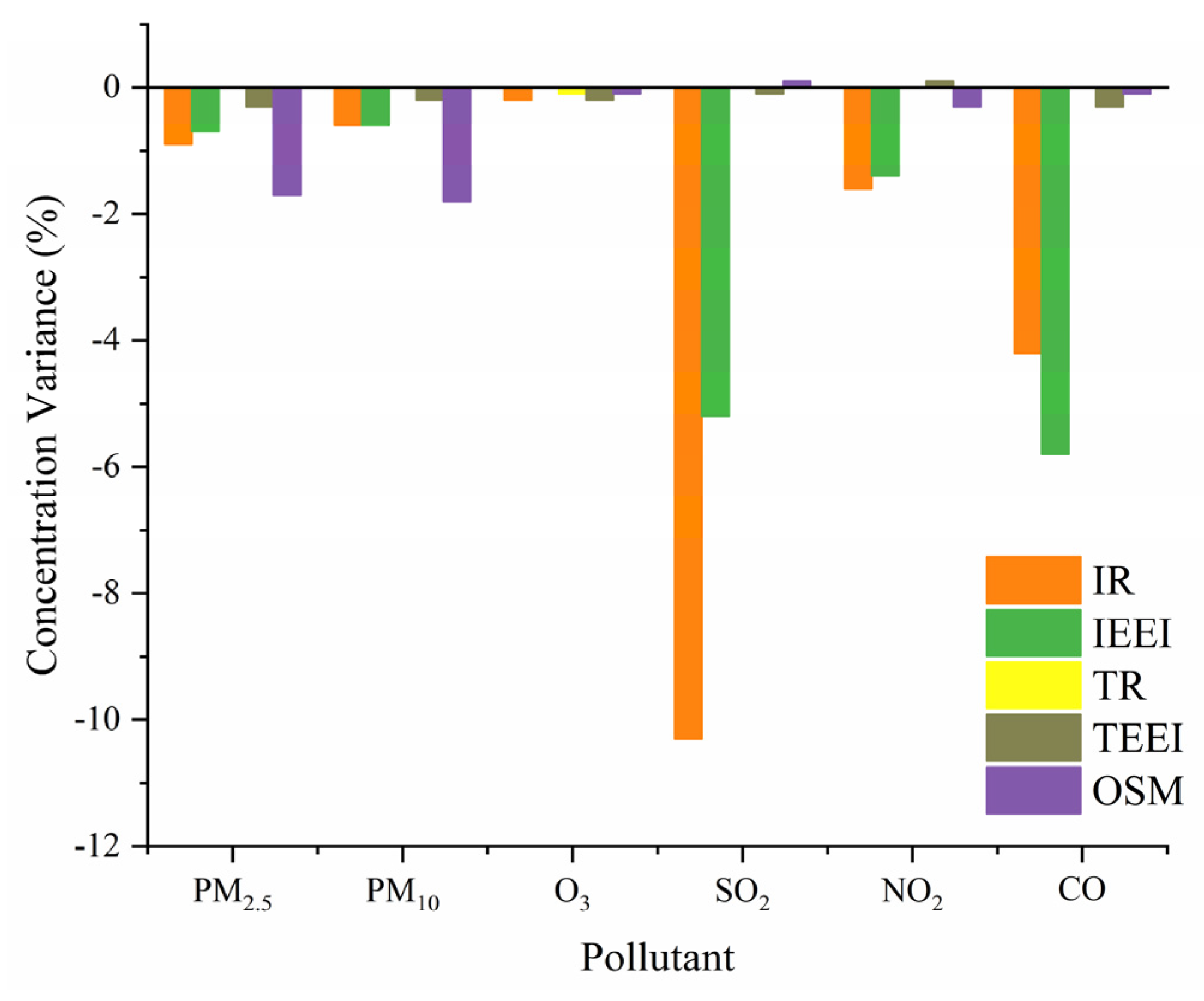
| Scenarios | PM2.5 | PM10 | O3 | SO2 | NO2 | CO |
|---|---|---|---|---|---|---|
| IR | −0.90% | −0.60% | −0.20% | −10.30% | −1.60% | −4.20% |
| IEEI | −0.70% | −0.60% | 0.00% | −5.20% | −1.40% | −5.80% |
| TR | 0.00% | 0.00% | −0.10% | 0.00% | 0.00% | 0.00% |
| TEEI | −0.30% | −0.20% | −0.20% | −0.10% | 0.10% | −0.30% |
| OSM | −1.70% | −1.80% | −0.10% | 0.10% | −0.30% | −0.10% |
| Pollutants | Emission Reduction Intervals and Averages | Correlation Strength |
|---|---|---|
| SO2 | −0.1%~10.3% (3.1%) | 3 |
| CO | 0%~5.8% (2.08%) | 3 |
| PM2.5 | 0.3%~1.7% (0.72%) | 2 |
| NO2 | −0.1%~0.6% (0.64%) | 2 |
| PM10 | 0%~1.8% (0.64%) | 2 |
| O3 | 0%~0.2% (0.12%) | 1 |
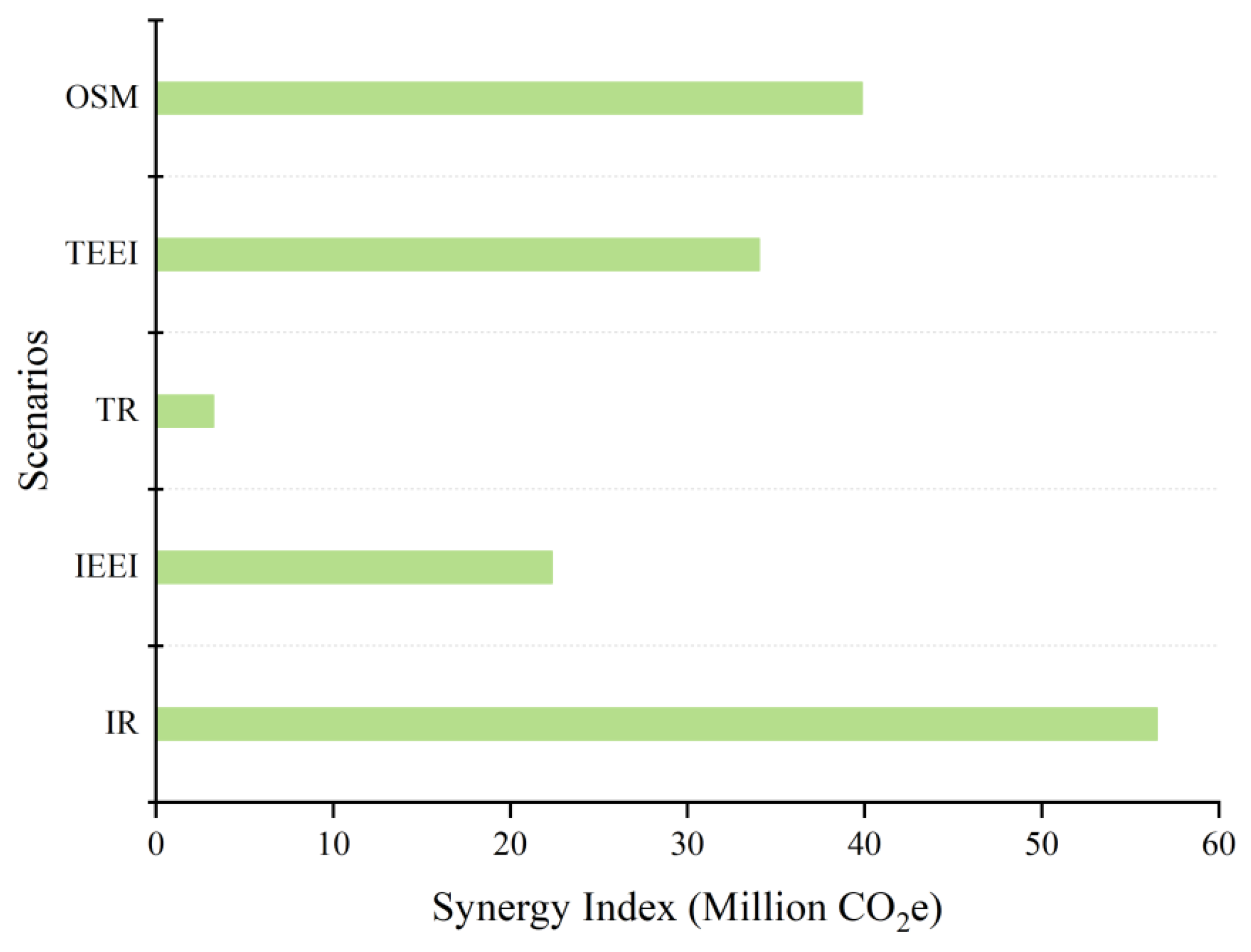
| Scenarios | AQCI | AQCI Improvement | Carbon Reduction (Kilotons CO2e) | Synergy Index (Carbon Reduction/AQCI Improvement) |
|---|---|---|---|---|
| IR | 2.63 | 0.043 | 2429.19 | 56,492.79 |
| IEEI | 2.59 | 0.085 | 1900.31 | 22,356.58 |
| TR | 2.67 | 0.003 | 9.73 | 3243.33 |
| TEEI | 2.67 | 0.004 | 136.11 | 34,027.50 |
| OSM | 2.65 | 0.022 | 876.71 | 39,850.45 |
Disclaimer/Publisher’s Note: The statements, opinions and data contained in all publications are solely those of the individual author(s) and contributor(s) and not of MDPI and/or the editor(s). MDPI and/or the editor(s) disclaim responsibility for any injury to people or property resulting from any ideas, methods, instructions or products referred to in the content. |
© 2023 by the authors. Licensee MDPI, Basel, Switzerland. This article is an open access article distributed under the terms and conditions of the Creative Commons Attribution (CC BY) license (https://creativecommons.org/licenses/by/4.0/).
Share and Cite
Wang, J.; Ma, J.; Wang, S.; Shu, Z.; Feng, X.; Xu, X.; Yin, H.; Zhang, Y.; Jiang, T. Coordination Relationship of Carbon Emissions and Air Pollutants under Governance Measures in a Typical Industrial City in China. Sustainability 2024, 16, 58. https://doi.org/10.3390/su16010058
Wang J, Ma J, Wang S, Shu Z, Feng X, Xu X, Yin H, Zhang Y, Jiang T. Coordination Relationship of Carbon Emissions and Air Pollutants under Governance Measures in a Typical Industrial City in China. Sustainability. 2024; 16(1):58. https://doi.org/10.3390/su16010058
Chicago/Turabian StyleWang, Junjie, Juntao Ma, Sihui Wang, Zhuozhi Shu, Xiaoqiong Feng, Xuemei Xu, Hanmei Yin, Yi Zhang, and Tao Jiang. 2024. "Coordination Relationship of Carbon Emissions and Air Pollutants under Governance Measures in a Typical Industrial City in China" Sustainability 16, no. 1: 58. https://doi.org/10.3390/su16010058
APA StyleWang, J., Ma, J., Wang, S., Shu, Z., Feng, X., Xu, X., Yin, H., Zhang, Y., & Jiang, T. (2024). Coordination Relationship of Carbon Emissions and Air Pollutants under Governance Measures in a Typical Industrial City in China. Sustainability, 16(1), 58. https://doi.org/10.3390/su16010058