


Grain Production in Turkey and Its Environmental Drivers Using ARDL in the Age of Climate Change


Abstract
:1. Introduction
2. Materials and Methods
2.1. Augmented Dickey and Fuller (ADF) and Phillips and Perron (PP) Tests
2.2. Cointegration Analysis: ARDL Bounds Test Approach
2.3. The Causality Test
3. Results
3.1. ARDL Bounds Test
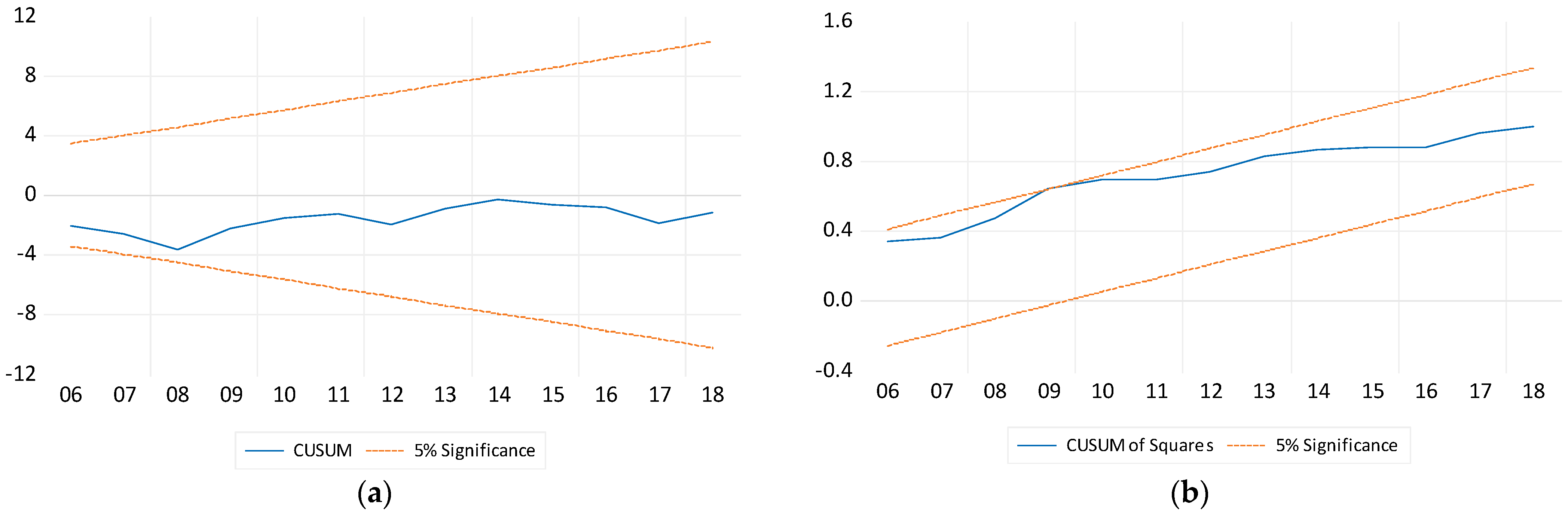
3.2. Diagnostic Tests
3.3. Toda–Yamamoto Causality Test
4. Discussion
5. Conclusions
Author Contributions
Funding
Institutional Review Board Statement
Informed Consent Statement
Data Availability Statement
Conflicts of Interest
References
- Tatlidil, F.; Boz, I.; Tatlidil, H. Farmers’ perception of sustainable agriculture and its determinants: A case study in Kahramanmaras province of Turkey. Environ. Dev. Sustain. 2009, 11, 1091–1106. [Google Scholar] [CrossRef]
- Gursoy, S.I. Addressing the challenge of food security in Turkey. In Environmental Law and Policies in Turkey. The Anthropocene: Politik-Economics-Society-Science; Savaşan, Z., Sümer, V., Eds.; Springer: Cham, Switzerland, 2020; Volume 31, pp. 127–140. [Google Scholar] [CrossRef]
- Dogan, H.P.; Aydogdu, M.H.; Sevinc, M.R.; Cancelik, M. Farmers’ willingness to pay for services to ensure sustainable agricultural income in the GAP-Harran plain, Şanlıurfa, Turkey. Agriculture 2020, 10, 152. [Google Scholar] [CrossRef]
- Yaman, H.M.; Ordu, B.; Zencirci, N.; Kan, M. Coupling socioeconomic factors and cultural practices in production of einkorn and emmer wheat species in Turkey. Environ. Dev. Sustain. 2020, 22, 8079–8096. [Google Scholar] [CrossRef]
- Henchion, M.; Hayes, M.; Mullen, A.M.; Fenelon, M.; Tiwari, B. Future protein supply and demand: Strategies and factors influencing a sustainable equilibrium. Foods 2017, 6, 53. [Google Scholar] [CrossRef] [PubMed]
- Namany, S.; Govindan, R.; Alfagih, L.; McKay, G.; Al-Ansari, T. Sustainable food security decision-making: An agent-based modelling approach. J. Clean. Prod. 2020, 255, 120296. [Google Scholar] [CrossRef]
- Turkstat. Labor Statistics. 2022. Available online: https://data.tuik.gov.tr/Bulten/Index?p=%C4%B0%C5%9Fg%C3%BCc%C3%BC-%C4%B0statistikleri-2021-45645anddil=1#:~:text=%C4%B0stihdam%C4%B1n%20%55%2C3’%C3%BC,ise%20hizmet%20sekt%C3%B6r%C3%BCnde%20yer%20ald%C4%B1 (accessed on 1 November 2023).
- Turkstat. Foreign Trade Statistics. 2022. Available online: https://data.tuik.gov.tr/Bulten/Index?p=Dis-Ticaret-Istatistikleri-Eylul-2022-45544anddil=1 (accessed on 1 November 2023).
- Johnston, B.F.; Mellor, J.W. The role of agriculture in economic development. Am. Econ. Rev. 1961, 51, 566–593. Available online: http://www.jstor.org/stable/1812786 (accessed on 21 November 2023).
- Josling, T.; Anderson, K.; Schmitz, A.; Tangermann, S. Understanding international trade in agricultural products: One hundred years of contributions by agricultural economists. Am. J. Agric. Econ. 2010, 92, 424–446. [Google Scholar] [CrossRef]
- Anderson, K. Agriculture’s globalization: Endowments, technologies, tastes, and policies. J. Econ. Surv. 2023, 37, 1314–1352. [Google Scholar] [CrossRef]
- Gutiérrez-Moya, E.; Adenso-Díaz, B.; Lozano, S. Analysis and vulnerability of the international wheat trade network. Food Secur. 2021, 13, 113–128. [Google Scholar] [CrossRef]
- Acibuca, V.; Kaya, A.; Kaya, T. Interregional comparative analysis of farmers’ perceptions and expectations of climate change. Ital. J. Agron. 2022, 17, 2121. [Google Scholar] [CrossRef]
- Cammarano, D. Climate variability and change impacts on crop productivity. Ital. J. Agron. 2022, 17, 2177. [Google Scholar] [CrossRef]
- Pathak, H.; Wassmann, R. Introducing greenhouse gas mitigation as a development objective in rice-based agriculture: I. genetation of technical coefficients. Agric. Syst. 2007, 94, 807–825. [Google Scholar] [CrossRef]
- Carriquiry, M.; Dumortier, J.; Elobeid, A. Trade scenarios compensating for halted wheat and maize exports from Russia and Ukraine increase carbon emissions without easing food insecurity. Nat. Food 2022, 3, 847–850. [Google Scholar] [CrossRef] [PubMed]
- Jagtap, S.; Trollman, H.; Trollman, F.; Garcia-Garcia, G.; Parra-López, C.; Duong, L.; Martindale, W.; Munekata, P.E.S.; Lorenzo, J.M.; Hdaifeh, A.; et al. The Russia-Ukraine conflict: Its implications for the global food supply chains. Foods 2022, 11, 2098. [Google Scholar] [CrossRef] [PubMed]
- Zhou, X.; Ma, W.; Li, G.; Qiu, H. Farm machinery use and maize yields in China: An analysis accounting for selection bias and heterogeneity. Aust. J. Agric. Resour. Econ. 2020, 64, 1282–1307. [Google Scholar] [CrossRef]
- Erenstein, O.; Jaleta, M.; Mottaleb, K.A.; Sonder, K.; Donovan, J.; Braun, H.J. Global Trends. Wheat Production, Consumption, and Trade. In Wheat Improvement; Reynolds, M.P., Braun, H.J., Eds.; Springer: Cham, Switzerland, 2022; pp. 47–66. [Google Scholar] [CrossRef]
- Takahashi, K.; Muraoka, R.; Otsuka, K. Technology adoption, impact, and extension in developing countries’ agriculture: A review of the recent literature. Agric. Econ. 2020, 51, 31–45. [Google Scholar] [CrossRef]
- Molotoks, A.; Smith, P.; Dawson, T.P. Impacts of land use, population, and climate change on global food security. Food. Energy Secur. 2021, 10, e261. [Google Scholar] [CrossRef]
- Krishna Bahadur, K.C.; Dias, G.M.; Veeramani, A.; Swanton, C.J.; Fraser, D.; Steinke, D.; Lee, E.; Wittman, H.; Farber, J.M.; Dunfield, K.; et al. When too much isn’t enough: Does current food production meet global nutritional needs? PLoS ONE 2018, 13, e0205683. [Google Scholar] [CrossRef]
- Aybek, A.; Kuzu, H.; Karadol, H. Evaluation for the Last Ten Years (2010–2019) and Next Years (2020–2030) of Changes in the Agricultural Mechanization Level of Turkey and the Agricultural Regions KSU. J. Agric. Nat. 2021, 24, 319–336. [Google Scholar] [CrossRef]
- Grey, D.; Sadoff, W.S. Sink or Swim? Water security for growth and development. Water Policy 2007, 9, 545–571. [Google Scholar] [CrossRef]
- Seddon, N.; Smith, A.; Smith, P.; Key, I.; Chausson, A.; Girardin, C.; House, J.; Srivastava, S.; Turner, B. Getting the message right on nature-based solutions to climate change. Glob. Chang. Biol. 2021, 27, 1518–1546. [Google Scholar] [CrossRef] [PubMed]
- Liao, W.; Zeng, F.; Chanieabate, M. Mechanization of small-scale agriculture in China: Lessons for enhancing smallholder access to agricultural machinery. Sustainability 2022, 14, 7964. [Google Scholar] [CrossRef]
- Gokdogan, O. Comparison of Indicators of Agricultural Mechanization Level of Turkey and the European Union; Adnan Menderes Universitesi Ziraat Fakultesi Dergisi: Koçarlı/Aydın, Türkiye, 2012; Volume 9, pp. 1–4. Available online: https://dergipark.org.tr/tr/pub/aduziraat/issue/26423/278160 (accessed on 21 November 2023).
- Agarwal, B. Gender equality, food security, and sustainable development goals. Curr. Opin. Environ. Sustain. 2018, 34, 26–32. [Google Scholar] [CrossRef]
- Devi, M.; Kumar, J.; Malik, D.; Mishra, P. Forecasting of wheat production in Haryana using a hybrid time series model. J. Agric. Food Res. 2021, 5, 100175. [Google Scholar] [CrossRef]
- FAO. Faostat. 2022. Available online: https://www.fao.org/faostat/en/#dat (accessed on 6 November 2023).
- World Bank. Fertilizer Consumption (Kilograms per Hectare of Arable Land). Available online: https://data.worldbank.org/indicator/AG.CON.FERT.ZS (accessed on 12 November 2023).
- Weldeslassie, T.; Naz, H.; Singh, B.; Oves, M. Chemical contaminants for soil, air and aquatic ecosystem. In Modern Age Environmental Problems and Their Remediation, 2nd ed.; Oves, M., Zain Khan, M., Ismail, I.M.I., Eds.; Springer: Cham, Switzerland, 2018; pp. 1–22. [Google Scholar] [CrossRef]
- Rehman, A.; Ma, H.; Ozturk, I. Decoupling the climatic and carbon dioxide emission influence to maize crop production in Pakistan. Air Qual. Atmos. Health 2020, 13, 695–707. [Google Scholar] [CrossRef]
- Abate, M.C.; Kuang, Y.P. The impact of the supply of farmland, level of agricultural mechanization, and supply of rural labor on grain yields in China. Stud. Agric. Econ. 2021, 123, 33–42. [Google Scholar] [CrossRef]
- Ahsan, F.; Chandio, A.A.; Fang, W. Climate change impacts cereal crop production in Pakistan: Evidence from cointegration analysis. Int. J. Clim. Chang. Strateg. Manag. 2020, 12, 257–269. [Google Scholar] [CrossRef]
- Ali, S.; Ying, L.; Shah, T.; Tariq, A.; Chandio, A.; Ali, I. Analysis of the nexus of CO2 emissions, economic growth, land under cereal crops, and agriculture value-added in Pakistan using an ARDL approach. Energies 2019, 12, 4590. [Google Scholar] [CrossRef]
- Chandio, A.A.; Jiang, Y.; Rehman, A. Using the ARDL-ECM approach to investigate the nexus between support price and wheat production: An empirical evidence from Pakistan. J. Asian Bus. Econ. Stud. JABES 2019, 26, 139–152. [Google Scholar] [CrossRef]
- Chandio, A.A.; Ozturk, I.; Akram, W.; Ahmad, F.; Mirani, A.A. Empirical analysis of climate change factors affecting cereal yield: Evidence from Turkey. Environ. Sci. Pollut. Res. 2020, 27, 11944–11957. [Google Scholar] [CrossRef]
- Chopra, R.R. Sustainability assessment of crops’ production in India: Empirical evidence from ARDL-ECM approach. J. Agribus. Dev. Emerg. 2022, 13, 468–489. [Google Scholar] [CrossRef]
- Koondhar, M.A.; Aziz, N.; Tan, Z.; Yang, S.; Abbasi, K.R.; Kong, R. Green growth of cereal food production under the constraints of agricultural carbon emissions: A new insights from ARDL and VECM models. Sustain. Energy. Technol. Assess. 2021, 47, 101452. [Google Scholar] [CrossRef]
- Kumar, P.; Sahu, N.C.; Kumar, S.; Ansari, M.A. Impact of climate change on cereal production: Evidence from lower-middle-income countries. Environ. Sci. Pollut. Res. 2021, 28, 51597–51611. [Google Scholar] [CrossRef]
- Ramzan, M.; Iqbal, H.A.; Usman, M.; Ozturk, I. Environmental pollution and agricultural productivity in Pakistan: New insights from ARDL and wavelet coherence approaches. Environ. Sci. Pollut. Res. 2022, 29, 28749–28768. [Google Scholar] [CrossRef] [PubMed]
- Yurtkuran, S. The effect of agriculture, renewable energy production, and globalization on CO2 emissions in Turkey: A bootstrap ARDL approach. Renew. Energy 2021, 171, 1236–1245. [Google Scholar] [CrossRef]
- Amponsah, L.; Kofi Hoggar, G.; Yeboah Asuamah, S. Climate Change and Agriculture: Modeling the Impact of Carbon Dioxide Emission on Cereal Yield in Ghana. Munich Pers. RePEc Arch. MPRA 2015, 2, 32–38. Available online: https://ideas.repec.org/p/pra/mprapa/68051.html (accessed on 6 November 2023).
- Zhao, C.; Liu, B.; Piao, S.; Wang, X.; Lobell, D.B.; Huang, Y.; Huang, M.; Yao, Y.; Bassu, S.; Ciais, P.; et al. Temperature increase reduces global yields of major crops in four independent estimates. Proc. Natl. Acad. Sci. USA 2017, 114, 9326–9331. [Google Scholar] [CrossRef] [PubMed]
- Dickey, D.A.; Fuller, W.A. Likelihood ratio statistics for autoregressive time series with a unit root. Econometrica 1981, 49, 1057–1072. [Google Scholar] [CrossRef]
- Phillips, P.; Perron, P. Testing for a unitroot in time series regression. Biometrika 1988, 75, 335–346. [Google Scholar] [CrossRef]
- Engle, R.F.; Granger, C.W.J. Cointegration and error correction: Representation, estimation, and testing. Econometrica 1987, 55, 251–276. [Google Scholar] [CrossRef]
- Johansen, S. Statistical analysis of cointegration vectors. J. Econ. Dyn. Control JEDC 1988, 12, 231–254. [Google Scholar] [CrossRef]
- Johansen, S.; Juselius, K. Maximum likelihood estimation and inference on cointegration with applications to the demand for money. Oxf. Bull. Econ. Stat. 1990, 52, 169–210. [Google Scholar] [CrossRef]
- Pesaran, M.H.; Shin, Y.; Smith, R.J. Bounds testing approaches to the analysis of level relationships. J. Appl. Econ. 2001, 16, 289–326. [Google Scholar] [CrossRef]
- Tang, T.C. Japanese aggregate import demand function: Reassessment from the bounds testing approach. Jpn. World Econ. 2003, 15, 419–436. [Google Scholar] [CrossRef]
- Narayan, S.; Narayan, P.K. Determinants of demand for Fiji’s exports: An empirical investigation. Dev. Econ. 2004, 42, 95–112. [Google Scholar] [CrossRef]
- Narayan, P.K. The saving and investment nexus for China: Evidence from cointegration tests. Appl. Econ. 2005, 37, 1979–1990. [Google Scholar] [CrossRef]
- Brown, R.L.; Durbin, J.; Evans, J.M. Techniques for testing the constancy of regression relationships over the time-with discussion. J. R. Stat. Soc. Ser. B 1975, 37, 149–192. [Google Scholar]
- Granger, C.W. Investigating causal relations by econometric models and cross-spectral methods. Econometrica 1969, 37, 424–438. [Google Scholar] [CrossRef]
- Toda, H.Y.; Yamamoto, T. Statistical inference in vector auto regressions with possibly integrated processes. J. Econ. 1995, 66, 225–250. [Google Scholar] [CrossRef]
- Gul, A.; Chandio, A.A.; Siyal, S.A.; Rehman, A.; Xiumin, W. How climate change is impacting the major yield crops of Pakistan? An exploration from long-and short-run estimation. Environ. Sci. Pollut. Res. 2022, 29, 26660–26674. [Google Scholar] [CrossRef]
- Chandio, A.A.; Jiang, Y.; Amin, A.; Akram, W.; Ozturk, I.; Sinha, A.; Ahmad, F. Modeling the impact of climatic and non-climatic factors on cereal production: Evidence from Indian agricultural sector. Environ. Sci. Pollut. Res. 2022, 29, 14634–14653. [Google Scholar] [CrossRef] [PubMed]
- Chandio, A.A.; Jiang, Y.; Akram, W.; Adeel, S.; Irfan, M.; Jan, I. Addressing the effect of climate change in the framework of financial and technological development on cereal production in Pakistan. J. Clean. Prod. 2021, 288, 125637. [Google Scholar] [CrossRef]
- Trademap. Trade Statistics for International Business Development, Monthly, Quarterly and Yearly Trade Data. Import and Export Values, Volumes, Growth Rates, Market Shares, etc. Available online: https://www.trademap.org/Index.aspx (accessed on 6 November 2023).
- Eroglu, N.A.; Bozoglu, M.; Bilgic, A. The impact of livestock supports on production and income of the beef cattle farms: A case of Samsun Province, Turkey. J. Agric. Sci. 2019, 26, 117–129. [Google Scholar] [CrossRef]
- Tan, M.; Yolcu, H. Current status of forage crops cultivation and strategies for the future in Turkey: A review. J. Agric. Sci. 2021, 27, 114–121. [Google Scholar] [CrossRef]
- Koondhar, M.A.; Udemba, E.N.; Cheng, Y.; Khan, Z.A.; Koondhar, M.A.; Batool, M.; Kong, R. Asymmetric causality among carbon emission from agriculture, energy consumption, fertilizer, and cereal food production—A nonlinear analysis for Pakistan. Sustain. Energy Technol. Assess. 2021, 45, 101099. [Google Scholar] [CrossRef]
- FAO. The State of Food Security and Nutrition in the World. In Repurposing Food and Agricultural Policies to Make Healthy Diets More Affordable; FAO: Rome, Italy, 2022. [Google Scholar] [CrossRef]
- FAO. Climate Change and Food Security: Risks and Responses. 2015. Available online: www.fao.org/publications (accessed on 18 November 2023).
- Warsame, A.A.; Sheik-Ali, I.A.; Ali, A.O.; Sarkodie, S.A. Climate change and crop production nexus in Somalia: An empirical evidence from ARDL technique. Environ. Sci. Pollut. Res. 2021, 28, 19838–19850. [Google Scholar] [CrossRef]
- Pickson, R.B.; He, G.; Ntiamoah, E.B.; Li, C. Cereal production in the presence of climate change in China. Environ. Sci. Pollut. Res. 2020, 27, 45802–45813. [Google Scholar] [CrossRef]

| Author(s) | Method | Variables and Their Descriptions | The Dependent Variable | Relationship −/+ (Long Term) | Country, Period |
|---|---|---|---|---|---|
| Abate and Kuang [34] | ARDL | OGC = Output of Grain Crops TNREL = Total Number of Employed Rural Labor, AGC = Total Sown Area of Grain Crops, TPAM = Total Power of Agricultural Machinery | OGC | TNREL (+), AGC (+), PAM (+) | China, 1978–2012 |
| Ahsan et al. [35] | Johansen cointegration test, ARDL, Granger | CP = Cereal Crops Production, CO2 = Carbon Dioxide Emissions, EN = Energy Consumption, CA = Cultivated Area, LF = Labor Force | CP | CO2 (+), CA (+), EN (+), LF (+) | Pakistan, 1971–2014 |
| Ali et al. [36] | Johansen cointegration test, ARDL | CO2 = Carbon Dioxide Emissions, GDP = Gross Domestic Product, LCC = Land Under Cereal Crop, AVA = Agriculture Value Added | CO2 | LCC (+), GDP (+), AVA (−) | Pakistan, 1961–2014 |
| Chandio et al. [37] | ARDL, ECM | WP = Wheat Production, AR = Area Under Cultivation, SP = Support Price, FC = Fertilizer Consumption | WP | AR (+), SP(+), FC (+) | Pakistan, 1971–2016 |
| Chandio et al. [38] | ARDL | YC = Yield of Cereal Crop, CO2 = CO2 Emissions Per Capita, AT = Average Temperature, AR = Average Rainfall, LCP = Land Under Cereal Production, EC = Energy Consumption, LAB = Labor Force | YC | CO2 (−) | Turkey, 1968–2014 |
| Chopra [39] | ARDL, ECM, FMOLS, DOLS | TP = Total Crop Production, LU = Cultivable Land Use, AWU = Agricultural Water Use, GIA = Gross Irrigated Area, AR = Annual Rainfall, Tmax = Maximum Temperature and Tmin = Minimum Temperature. | TP | LU (+), GIA (+) | India, 1960–2015 |
| Koondhar et al. [40] | ARDL, VECM, Granger | CFP = Cereal Food Production, AS = Area Sown, ACO2 = Agricultural CO2 Emissions, FPI = Food Production Index | CFP | AS (+), ACO2 (−) | China, 1985–2018 |
| Kumar et al. [41] | FMOLS, DOLS | CP = Cereal Production, AATD = Average Annual Temperature, AAR = Average Annual Rainfall, CO2 = Carbon Dioxide Emissions, LCP = Land Under Cereal Production, RPOP = Rural Population | CP | FGLS RESULT; CO2 (+), LCP (+), FMOLS RESULT; CO2 (+), LCP (+) | 1971–2016 Bangladesh, Ghana, India, Kenya, Myanmar, Nigeria, Phillippines, Sri Lanka, Vietnam, Indonesia, and Pakistan |
| Ramzan et al. [42] | ARDL, WTC, Toda–Yamamoto | TFP = Total Agricultural Productivity (Index Value), ALB = Agricultural Labor, ALD = Agricultural Land, FD = Agricultural Feed, FT = Fertilizer, CO2 = Carbon Dioxide Emissions | TFP | ALB (+), ALD (+), FD (+), FD (+), FT (+), CO2 (+) | Pakistan, 1961–2018 |
| Rehman et al. [33] | ARDL, Granger | CO2 = Carbon Dioxide Emissions, MCP = Maize Crop Production, AMC = Area Under Maize Crop, WA = Water Availability, RF = Rainfall and TM = Temperature | CO2 | MCP (+), WA (+), RF (+), TM (+), AMC (−) | Pakistan, 1988–2017 |
| Yurtkuran [43] | Gregory Hansen cointegration test, ARDL | CO2 = Carbon Dioxide Emissions, REN = Renewable Energy Production, AGR = Agriculture (% of GDP); and KOFE, KOFS, and KOFP represent the economic, social, and political KOF globalization indices, respectively | CO2 | AGR (+), REN (+), KOFE (+) | Türkiye, 1970–2017 |
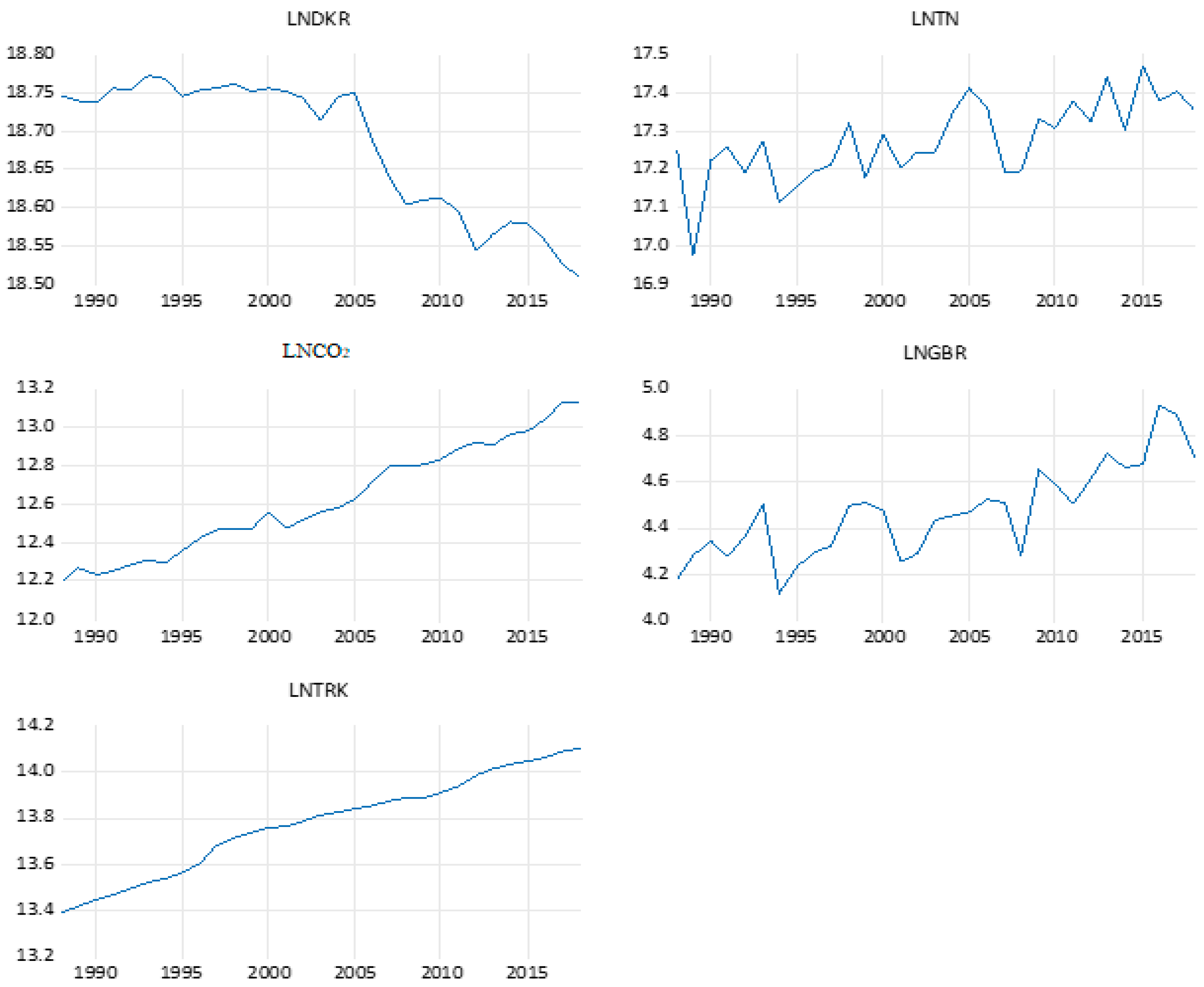
| Abbreviations | Variable | Measurement | Sources |
|---|---|---|---|
| DKR | Area Under Cultivation of Grain Crops | Million hectares | TURKSTAT |
| TON | Amount of Grain Production | Kg per hectare | TURKSTAT |
| GBR | Fertilizer Consumption | Kg per hectare of arable land | WorldBank |
| TRK | Number of Trucks | Unit | TURKSTAT |
| CO2 | Agricultural Greenhouse Gas Emissions | Gigagrams | WorldBank |
| Variables | ADF | PP | ||
|---|---|---|---|---|
| Level | 1st Difference | Level | 1st Difference | |
| lnDKR | −3.850819 (0.0004) *** | −3.903828 (0.0003) *** | ||
| lnTON | −4.334403 (0.0098) *** | −14.76907 (0.0000) *** | ||
| lnCO2 | −6.391589 (0.0000) *** | −6.550400 (0.0000) *** | ||
| lnGBR | −4.337709 (0.0091) *** | −4.337709 (0.0091) *** | ||
| lnTRAK | −3.553848 (0.0135) ** | −3.429667 (0.0180) ** | ||
| Test | F-Stat | Probability | Result |
|---|---|---|---|
| Breusch–Godfrey serial correlation LM test | 2.087005 | 0.1705 | No problem with serial correlations |
| Breusch–Pagan–Godfrey heteroscedasticity test | 1.7011 | 0.173 | No problem of heteroscedasticity |
| Jarque–Bera test | 1.026939 | 0.598416 | The estimated residual is normal |
| Ramsey test | 0.100048 | 0.7572 | The model is specified correctly |
| Long-Run | |||
| Variable | Coefficient | t statistic | Prob. |
| lnTON | −0.299075 ** | −2.852220 | 0.0136 |
| lnCO2 | −0.776908 *** | −15.38627 | 0.0000 |
| lnGBR | 0.106338 ** | 2.584972 | 0.0226 |
| lnTRK | 0.638938 *** | 10.56377 | 0.0000 |
| Short-Run | |||
| Variable | Coefficient | t statistic | Prob. |
| C | 23.19385 *** | 7.943460 | 0.0000 |
| D(lnDKR(−1)) | 0.452619 *** | 3.434853 | 0.0044 |
| D(lnTON) | −0.003477 | −0.106257 | 0.9170 |
| D(lnTON(−1)) | 0.130862 *** | 4.149396 | 0.0011 |
| D(lnTON(−2)) | 0.049165 * | 2.060700 | 0.0599 |
| D(lnCO2) | −0.10276 * | −1.921108 | 0.0769 |
| D(lnCO2(−1)) | 0.441496 *** | 4.422994 | 0.0007 |
| D(lnCO2(−2)) | 0.2710509 *** | 4.099552 | 0.0013 |
| D(lnGBR) | 0.034123 * | 2.000659 | 0.0668 |
| D(lnTRK) | −0.118232 | −0.843892 | 0.4140 |
| CointEq(−1) | −0.952379 *** | −7.943820 | 0.0000 |
| Sensitivity Analysis | |||
| R2 | 0.901617 | ||
| Adjusted R2 | 0.843744 | ||
| F statistic | 15.57936 | ||
| Prob (F statistic) | 0.000001 | ||
| Durbin-Watson stat | 2.354542 | ||
| Test | F-Stat | Probability | Result |
|---|---|---|---|
| Breusch–Godfrey serial correlation LM test | 2.087005 | 0.1705 | No problem with serial correlations |
| Breusch–Pagan–Godfrey heteroscedasticity test | 1.701100 | 0.1730 | No problem of heteroscedasticity |
| Jarque–Bera test | 1.026939 | 0.598416 | The estimated residual is normal |
| Ramsey test | 0.100048 | 0.7572 | The model is specified correctly |
| Variable | lnDKR | lnTON | lnCO2 | lnGBR | lnTRK |
|---|---|---|---|---|---|
| lnDKR | - | 6.493 *** (0.010) | - | - | 2.692 * (0.100) |
| lnTN | 16.200 *** (0.000) | - | 8.156 *** (0.004) | 4.040 ** (0.044) | - |
| lnCO2 | 28.436 *** (0.000) | - | - | - | 4.636 ** (0.031) |
| lnGBR | 8.487 *** (0.003) | - | 2.709 * (0.099) | - | 6.849 *** (0.008) |
| lnTRK | 28.031 *** (0.000) | 6.461 ** (0.011) | - | - | - |
lnTON  lnDKR lnDKR | lnTRK  lnTN lnTN | lnTON lnGBR | |||
| lnCO2 lnDKR | lnTON lnCO2 | lnCO2 lnTRK | |||
| lnGBR lnDKR | lnGBR lnCO2 | lnGBR lnTRK | |||
| lnTRK lnDKR | |||||
Disclaimer/Publisher’s Note: The statements, opinions and data contained in all publications are solely those of the individual author(s) and contributor(s) and not of MDPI and/or the editor(s). MDPI and/or the editor(s) disclaim responsibility for any injury to people or property resulting from any ideas, methods, instructions or products referred to in the content. |
© 2023 by the authors. Licensee MDPI, Basel, Switzerland. This article is an open access article distributed under the terms and conditions of the Creative Commons Attribution (CC BY) license (https://creativecommons.org/licenses/by/4.0/).
Share and Cite
Gurbuz, I.B.; Kadioglu, I. Grain Production in Turkey and Its Environmental Drivers Using ARDL in the Age of Climate Change. Sustainability 2024, 16, 264. https://doi.org/10.3390/su16010264
Gurbuz IB, Kadioglu I. Grain Production in Turkey and Its Environmental Drivers Using ARDL in the Age of Climate Change. Sustainability. 2024; 16(1):264. https://doi.org/10.3390/su16010264
Chicago/Turabian StyleGurbuz, Ismail Bulent, and Irfan Kadioglu. 2024. "Grain Production in Turkey and Its Environmental Drivers Using ARDL in the Age of Climate Change" Sustainability 16, no. 1: 264. https://doi.org/10.3390/su16010264
APA StyleGurbuz, I. B., & Kadioglu, I. (2024). Grain Production in Turkey and Its Environmental Drivers Using ARDL in the Age of Climate Change. Sustainability, 16(1), 264. https://doi.org/10.3390/su16010264