Article

Multi-Site and Multi-Pollutant Air Quality Data Modeling

1
School of Finance, Southwestern University of Finance and Economics, Chengdu 610074, China
2
Center of Statistical Research, School of Statistics, Southwestern University of Finance and Economics, Chengdu 610074, China
3
Department of Statistics and Actuarial Science, The University of Hong Kong, Hong Kong, China
*
Author to whom correspondence should be addressed.
Sustainability 2024, 16(1), 165; https://doi.org/10.3390/su16010165
Submission received: 10 November 2023 / Revised: 4 December 2023 / Accepted: 19 December 2023 / Published: 23 December 2023
(This article belongs to the Section Air, Climate Change and Sustainability)

Abstract

:
This study proposes a new method for predicting air quality in major industrialized cities around the world. In some big cities, multiple air quality measurement stations are deployed at different locations to monitor air pollutants, such as NO2, CO, PM 2.5, and PM 10, over time. At every monitoring timestamp t, we observe one station × feature matrix x t of the pollutant data, which represents a spatio-temporal process. Traditional methods of prediction of air quality typically use data from one station or can only predict a single pollutant (such as PM 2.5) at a time, which ignores the spatial correlation among different stations. Moreover, the air pollution data are typically highly non-stationary. This study has explicitly overcome the limitations of these two aspects, forming its unique contributions. Specifically, we propose a de-trending graph convolutional LSTM (long short-term memory) to continuously predict the whole station × feature matrix in the next 1 to 48 h, which not only captures the spatial dependency among multiple stations by replacing an inner product with convolution, but also incorporates the de-trending signals (transforms a non-stationary process to a stationary one by differencing the data) into our model. Experiments on the air quality data of the city of Chengdu and multiple major cities in China demonstrate the feasibility of our method and show promising results.

1. Introduction

The air quality problem is not only a health issue but also an urgent issue for sustainable development. With the rapid development of the global economy, the challenge of air pollution has become increasingly apparent. Air quality issues are complex and receive increasing attention. In most cities, multiple monitoring stations are located at different locations to report air quality indicators in real-time. Typically, levels of air pollutants are recorded hourly by multiple stations (such as the data used in this article). This means that at every timestamp, one air quality matrix with the shape of station × feature can be collected by all the stations, where features include NO2, CO, PM2.5, PM10, etc. Based on this air quality data matrix, an air quality index (AQI) can be calculated to inform the public of the air quality at present [1]. However, the general public is more interested in predicting future air quality rather than real-time reporting. This prediction not only benefits people’s daily activities (such as developing travel plans or avoiding routes with poor air quality), but also improves their health by wearing masks to reduce exposure to air pollution. It also provides policy implications for the government.
There are a large number of works for air quality prediction in the literature [2,3,4,5,6]. Most of them are based on the temporal dependency between future states and historical data, such as time series models [4,7,8] and deep neural networks [3,9,10,11]. However, there are several limitations to the existing methods. First, many models [4,9,10] take the air quality prediction as a single-pollutant regression problem; for example, focusing on only the particulate matter PM2.5. To predict the level of another pollutant, e.g., carbon monoxide CO, a different model needs to be trained. Second, to improve the performance for prediction, some methods [8,12] choose to incorporate extra knowledge, such as the weather forecasting results [12] or the traffic data [8]. In practical applications, it is not convenient to collect additional information and synchronize it with air quality data. When data from multiple stations are available, the geographic correlation between these stations is expected to contribute to air quality prediction [8,12]. However, most existing methods can only process data from one station at a time, leaving spatial correlations between multiple stations ignored [3,4,10] or partially considered [8,
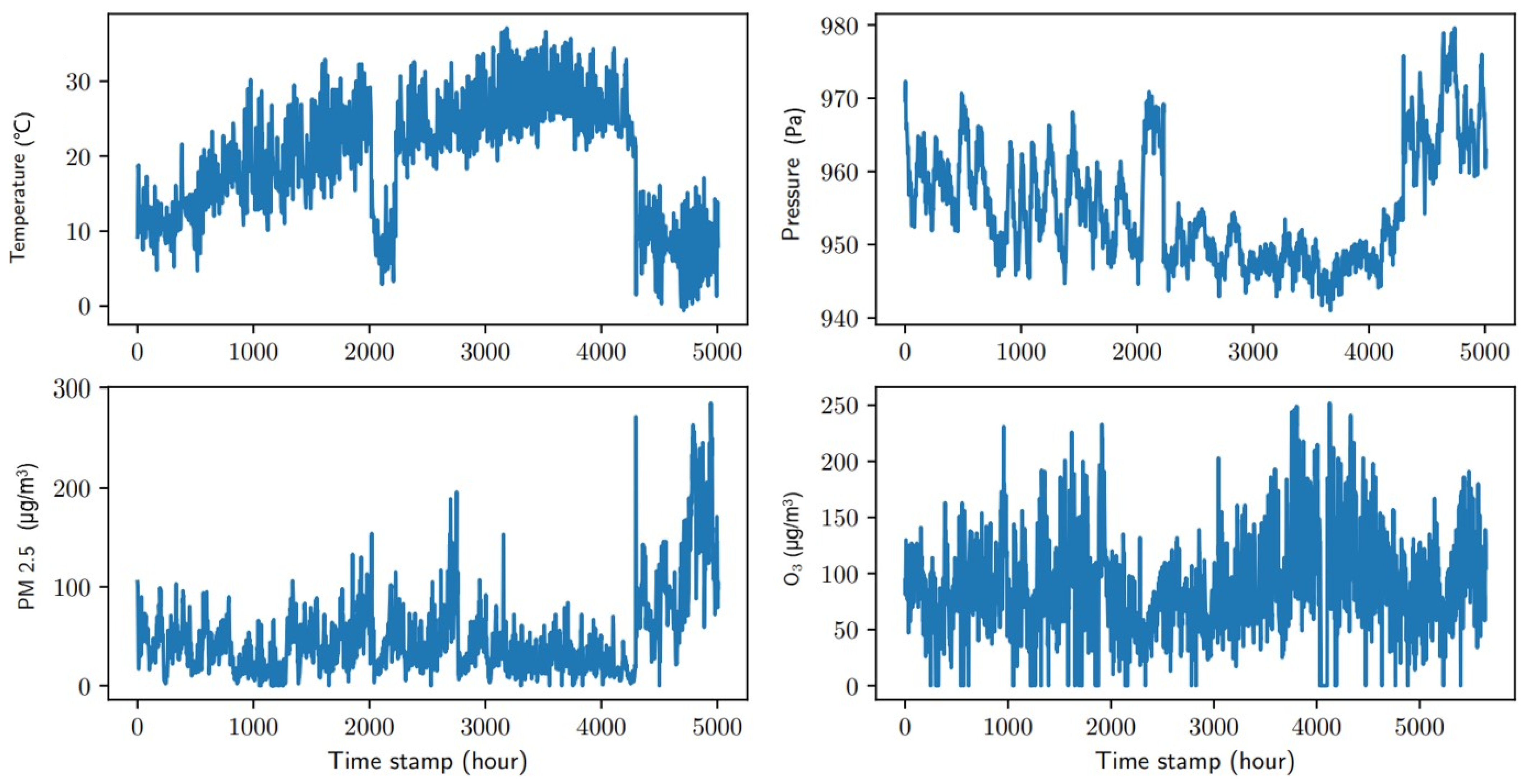
12]. Last but not least, air quality data usually represent a high degree of non-stationarity, as shown in Figure 1, where the mean value of the data varies over time, making the modeling problem even more difficult. Ignoring the non-stationarity in the data can lead to unacceptable prediction errors and severely weaken the predictive power of the model. Therefore, learning potential spatio-temporal features from non-smooth processes is particularly important for prediction.
We propose to solve the aforementioned problems using a non-stationary diffusion graph convolutional LSTM (long short-term memory). In detail, the spatio–temporal characteristics of air quality data from multiple sites motivate us to use the diffusion convolutional LSTM network [13]. The diffusion convolution [14] captures the spatial dependency using bidirectional random walks on the meteorological monitoring sites graph G = ( V , E , A ) as shown in Figure 2b. In addition, we add a de-trending step to the diffusion convolutional LSTM to accommodate the non-stationarity of the data. This de-trending operation can better capture the true characteristics of the data, thus improving the accuracy of the prediction. In time series analysis, the de-trending step is usually implemented via a differencing procedure x t x t 1 [15,16]. As a result, the input of the proposed model involves both x t and x t x t 1 . We name the proposed model as the long–short de-trending graph convolutional network (LS-deGCN).
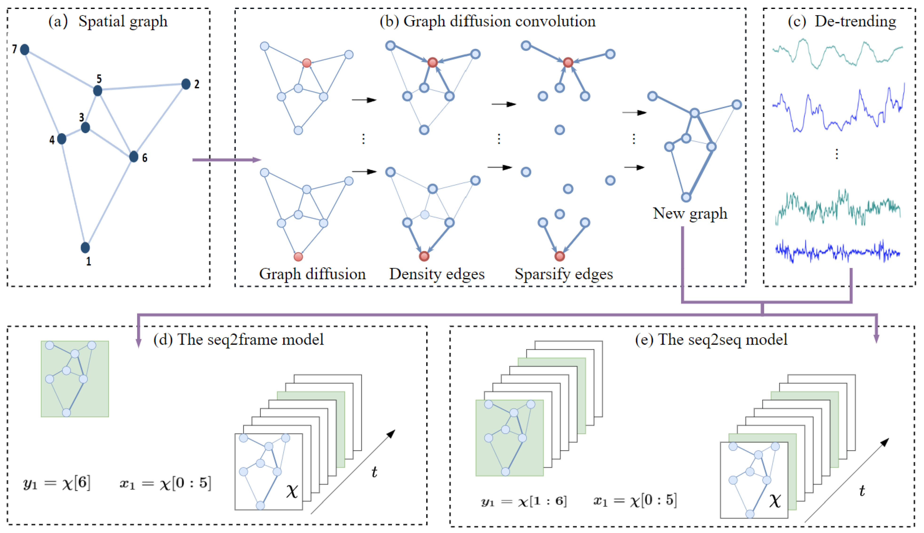
Motivated by the vast applications of LSTM in the area of natural language processing (NLP), we propose two variants of the LS-deGCN, as shown in Figure 3d,e. At every timestamp, there is one station × feature matrix of data x R M × N observed, where M is the number of stations and N is the number of features. Therefore, the final dataset is a three-dimensional tensor X R M × N × T by stacking all x ’s along the time, where T is the number of timestamps. Given a window length, for example, 3, which is a tuning parameter in our model, we can slice the samples along the third dimension T. For ease of exposition, we omit the first two dimensions and denote X [ 0 : 3 ] = X [ : , : , 0 : 3 ] . The sliced samples are in the form of x 1 = X [ 0 : 3 ] , x 2 = X [ 1 : 4 ] , etc. We propose two different ways of defining the target y , which correspond to the two variants of our models. One is a sequence-to-frame model, that is, y 1 = X [ 4 ] , y 2 = X [ 5 ] , etc., and the other is a sequence-to-sequence model, that is, y 1 = X [ 1 : 4 ] , y 1 = X [ 2 : 5 ] , etc.
The contributions of this research are threefold:
1.
Firstly, we introduce a de-trending operation into the traditional LSTM model to effectively eliminate the long-term trend in non-stationary data. This improvement enables our model to more accurately capture the changing patterns in non-stationary data.
2.
Secondly, we utilize a diffusion graph convolution to extract the spatial correlations present in the air quality data across multiple stations. This innovative method not only improves prediction accuracy, but also has important implications for understanding and predicting air pollutant spread and impacts.
3.
Lastly, we propose two distinct models based on LS-deGCN for multi-site air quality prediction and evaluate them on air quality data from Chengdu and seven other major cities. The experimental results demonstrate that the proposed models significantly outperform other existing methods in terms of prediction accuracy and stability.
The rest of the paper is structured as follows. Section 2 presents a brief review of related works and research gaps. In Section 3, we introduce the proposed LS-deGCN and its two variants: the sequence-to-frame model and the sequence-to-sequence model. The experimental results are shown in Section 4. Section 5 concludes this paper with some remarks.

2. Literature Review and Research Gaps

Traditionally, meteorologists often make air quality predictions based on their empirical knowledge of meteorology. With the development of statistics and machine learning, data-driven methods for air quality prediction are becoming increasingly popular nowadays, which can be typically divided into statistical approaches [4,17,18,19,20,21] and deep learning approaches [9,10,12,13,22,23].
Some existing deep learning models treat air quality forecasting as a single pollutant regression problem; thus, they only predict one pollutant at a time [4,9,24]. As a result, separate models need to be trained for different pollutants if all of the pollutants are of interest, where each model only focuses on one pollutant. Zhang et al. [4] conducted a statistical analysis of the PM2.5 data in the years 2013–2016 from the city of Beijing based on a flexible non-stationary hierarchical Bayesian model. Mukhopadhyay and Sahu [20] proposed a Bayesian spatio-temporal model to estimate the long-term exposure to air pollution levels in England. Since the air quality records are typically monitored over time, Ghaemi et al. [18] designed a LaSVM-based online algorithm to deal with the streaming of the air quality data. Along another direction, the Granger causality has been proposed to analyze the correlations among the air pollution sequences from different monitoring stations [7,8,12]. Suppose that the sequence of air pollutant records from one station is denoted by x t , and the sequence of a factor (such as the geographical correlation) from another station by y t , then the mathematical representation of the Granger causality is given by
x t = k = 1 K a k x t k + k = 1 K b k y t k + ϵ t ,
where a k is a weight indicating how the width of time window k affects the future evolution, b k represents the correspondent weight for x t and y t , and ϵ t is the residual for time series x t . If a k 0 and b k = 0 , it means that the sequence x t is caused by its own history. Wang and Song [12] combined the Granger causality with deep learning models and there are also some connections between the Granger causality and LSTM [25].
Deep learning, more specifically, the recurrent neural network (RNN) and LSTM [25] have achieved vast success in the area of NLP [26] and video analysis [27]. The LSTM can capture both the long and short contextual dependency of the data via different types of gates. In the classical LSTM, the well-designed gates, for example, the input gate and the forget gate, make the network very powerful to model the temporal correlations of the sequential data. Thus, much literature has applied LSTM and RNN to the field of air quality prediction.
Guo et al. [28] proposed a multi-variable LSTM based on both temporal- and variable-level attention mechanisms, which was used to predict the PM2.5 level in Beijing. Fan et al. [11] also used the LSTM as a framework to predict air quality in Beijing based on air pollution and meteorological information. Compared with [28], the data used in [11] are collected from multiple stations, while the data from different stations are analyzed separately by ignoring the spatial correlation. In big cities, there is usually more than one station deployed to monitor air pollutants and meteorological information. The correlations among readings from different stations are highly informative in forecasting future air quality; thus, the spatial information should be incorporated. Xu et al. [29] proposed a multi-scale three-dimensional tensor decomposition algorithm to deal with the spatio-temporal correlation in climate modeling. In deep learning, a convolutional neural network (CNN) has advantages in extracting spatial features, while the RNN has superior performance in processing sequence data. Therefore, it is expected to achieve more accurate prediction by combining convolution and RNN in the analysis of spatial and temporal data. Huang and Kuo [9] proposed to stack a CNN over LSTM to predict the level of PM2.5. However, this modification results in a non-time series model, which may result in a loss of power when quantifying sequential air quality data.
Although the classical RNN and LSTM possess powerful capabilities in modeling time series data, they may not be suitable to capture the spatial correlation in the air quality data [11]. Let us look at the specifics. The air quality data are hourly recorded by multiple stations. At each timestamp, the observed data can be represented by a station × feature matrix x R M × N , where M is the number of stations and N is the number of features. The features refer to air pollutants (e.g., CO2, PM
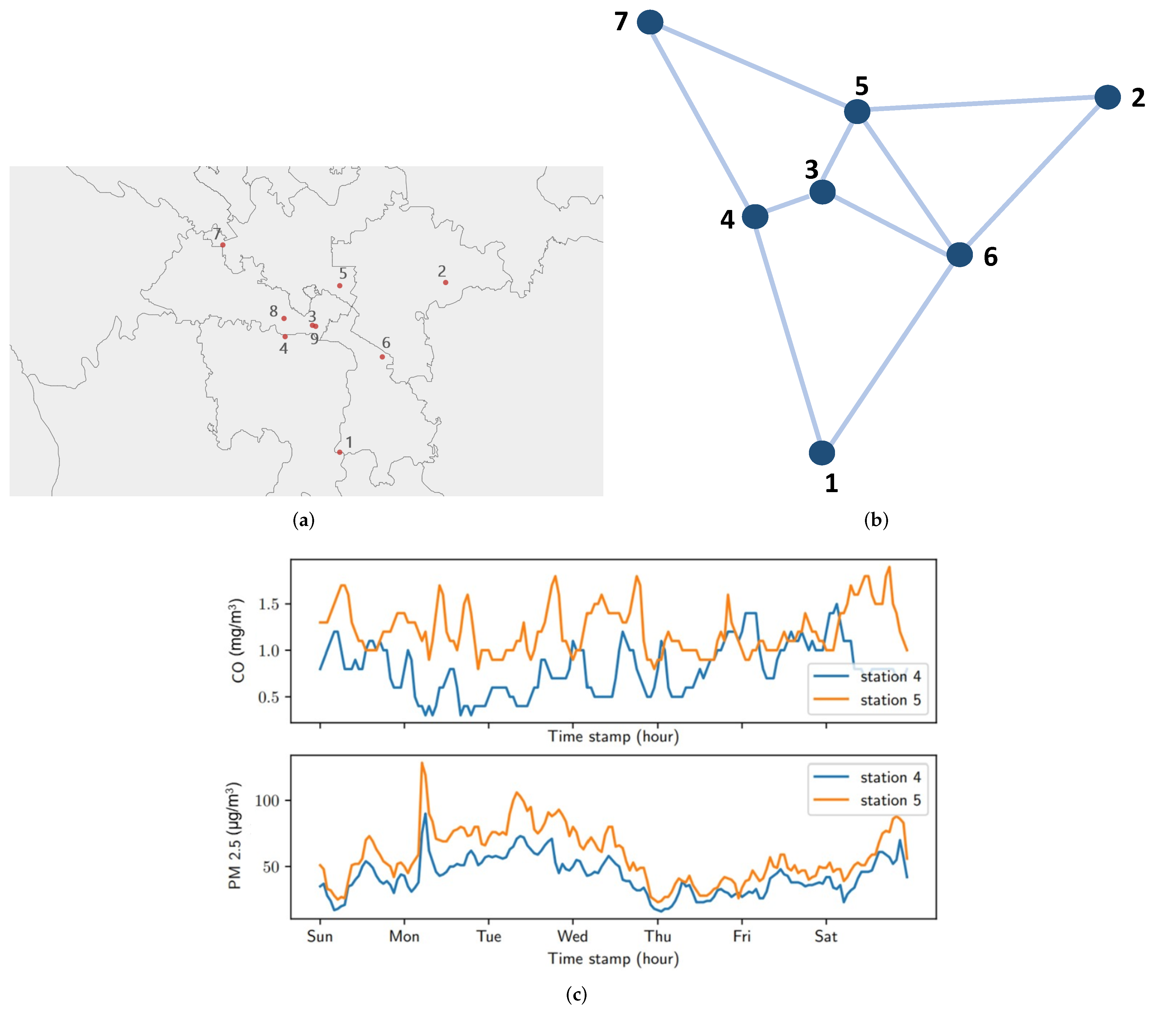
2.5) and meteorological parameters (e.g., air pressure, air temperature, and air humidity). As shown in Figure 2, the air quality data of the city of Chengdu involves nine monitoring stations and nine features. The entire data, thus, can be treated as a three-dimensional tensor X R M × N × T , with respect to the three axes station × feature × time. The third dimension T corresponds to the number of timestamps, which indicates the sequential nature of the data X .
The air quality data in Chengdu has a typical spatio-temporal patternn, and the data from different meteorological stations have a strong spatial correlation. Figure 2a shows the locations of different monitoring stations. Figure 2c shows the weekly readings of two types of pollutants, namely CO and PM2.5, from Station 4 and Station 5, respectively. In the records of CO and PM2.5, there is a significant change from four stations to five stations, and their patterns are similar. The area where Station 5 is located seems to be more polluted than the area where Station 4 is located, and this information is useful for government policy making in different regions. The similar oscillating patterns in the records of the two stations imply that the rows and columns in the matrix station × feature are correlated and further series correlation over time can also be observed. However, there seems no obvious daily periodicity or “weekends/holidays” effect from the data.
In this paper, we propose to model the air quality data from multiple stations with an LS-deGCN, which replaces the fully connected layer in the classical LSTM with graph diffusion convolution. According to the pairwise geographic distances between different stations, we compute the undirected graph G = ( V , E , A ) with a thresholded Gaussian kernel [30], where V, E, and A denote the vertex (station) set, edge set, and adjacent matrix of the graph, respectively. a i j = exp ( l i l j σ 2 ) , as shown in Figure 2b, where a i j is an element of the adjacent matrix A, l i and l j are the geographical locations of the i , j -th nodes, and l i l j calculates the distance between them. The LS-deGCN architecture can be well adapted to the spatio-temporal data. As far as we know, LS-deGCN was first proposed to analyze the two-dimensional radar echo map [13]. In addition, our model can accommodate the non-stationarity of the air quality data. Compared with the work of Wilson et al. [31], our method is easier to be implemented and trained. A similar diffusion convolutional recursive neural network was proposed in [14] to model the traffic flow.

3. Proposed Models

Figure 3 illustrates the overall framework of the proposed method.

3.1. Non-Stationary Diffusion Convolutional LSTM

We propose to model the non-stationary station × feature × time data with the de-trending diffusion convolutional LSTM (LS-deGCN), which aims to incorporate both the spatio-temporal correlations [13] and non-stationarity into our model. In contrast to the classical LSTM where all the gates are implemented via fully connected neural networks, the proposed model replaces them with diffusion operations [14]. In addition, the differences between the input signals x t x t 1 and corresponding hidden signals h t 1 h t 2 are input for de-trending as follows,
f t = σ W f [ x t , h t 1 ] + W d f [ x t x t 1 , h t 1 h t 2 ] + W c f c t 1 + b f
i t = σ W i [ x t , h t 1 ] + W d i [ x t x t 1 , h t 1 h t 2 ] + W c i c t 1 + b i
c t = f t c t 1 + i t tanh W c [ x t , h t 1 ] + W d c [ x t x t 1 , h t 1 h t 2 ] + b c
o t = σ W o [ x t , h t 1 ] + W d o [ x t x t 1 , h t 1 h t 2 ] + W c o c t + b o
h t = o t tanh c t ,
where * and ∘ represent the diffusion convolution and Hadamard product, respectively; [ a , b ] is the concatenation of vectors a and b ; σ ( · ) is the s i g m o i d function; and t a n h ( · ) is the hyperbolic tangent function. Equations (2), (3), and (5) correspond to the implementations of the forget gate, input gate, and output gate. Equation (4) is the updating mechanism of the cell state c t , and the hidden state h t is updated by Equation (6). Note that { W f , W d f , W c f , b f } are the weights (corresponding to the feature, de-trending term, and hidden state) and bias of the forget gate, and { W i , W d i , W c i , b i } and { W o , W d o , W c o , b o } are the counterparts of the input gate and the output gate, respectively. Furthermore, { W c , W d c , b c } are the weights (corresponding to the feature and de-trending term) and bias of the hidden state.
The diffusion graph convolution, which is shown in Figure 3b, is specifically designed to capture the diffusion process of information via the graph structure. This assumes that information is transferred from one node (monitoring station) to one of its neighbors (other monitoring stations) with a specific transfer probability, resulting in the information distribution reaching equilibrium after several iterations. This process facilitates information exchange and updates between nodes and their adjacent ones; moreover, it could incorporate information spread over multiple hops or steps in the graph, thereby enabling the capture of spatial correlations among different stations. The specific definition is as follows [14],
x ^ = m = 1 M k = 0 K 1 ( w k 1 ( D O 1 A ) k + w k 2 ( D I 1 A ) k ) x
where x is an input matrix and x ^ is the corresponding output. A is an adjacent matrix of the M stations as shown in Figure 2b, and D O and D I are the out-degree and in-degree diagonal matrix of A. D O 1 A and D I 1 A represent the transition matrices of the diffusion process and the reverse one, respectively.
The frame differencing term x t x t 1 is governed by the corresponding coefficient matrices. In Equation (5), we observe that not only does the current output o t depend on the current input x t , the current cell state c t , and the previous hidden state h t 1 , but it also requires the input of the differencing signal x t x t 1 . We also concatenate the hidden differencing signal h t 1 h t 2 with the input differencing x t x t 1 .
The main differences between the classical LSTM and our LS-deGCN lie in the diffusion graph convolutional operations and the extra de-trending items x t x t 1 and h t 1 h t 2 . If the graph convolution in Equations (2)–(6) are substituted with inner products and set x t x t 1 = 0 , h t 1 h t 2 = 0 , then the LS-deGCN reduces to the classical LSTM. The great success achieved by the graph convolutional neural network is largely owed to the graph convolution, which can effectively capture the spatial information of data. This is also the rationale underlying our LS-deGCN to characterize the spatial correlations.
As discussed earlier, the air quality data are typically collected from multiple stations over time, which represent both the spatial and temporal characteristics. The spatial correlations among different stations depend on many complicated factors such as geographical distances, directions, and meteorological features, which are very important for air quality prediction [7,8,12]. In the existing works, the spatial correlations are typically inferred manually by resorting to some complicated statistical processes. In this paper, we propose to model the spatial correlations with diffusion graph convolution. In other words, the spatial correlations among different stations can be extracted via the LS-deGCN, which is the most notable difference between our method and the existing models for air quality prediction. This distinctive feature makes our model coherent in the deep learning framework and more powerful for air quality forecasting.

3.2. Two New Models

According to the scheme of generating samples and targets as shown in Figure 3d,e, we develop two variants of our modeling framework. To help further elaboration, we first introduce some necessary notation. We first select Δ t , the width of a slicing window or the length of the samples, which is an analogy to the sentence length in NLP. The value of Δ t represents how many historical sample observations are used for prediction. Let l denote the time lag from a sample to the target; that is, our goal is to make a prediction of air quality for l hours later. We then propose the following two modeling frameworks.
In the sequence-to-frame (seq2frame) model, we take samples to be slices of the three-dimensional tensor X R M × N × T along the dimension T. The sample length is Δ t , the width of the slicing window. The target is taken to be the single frame after the corresponding samples. Since the time lag from a sample to its target is l, the training and testing samples can be generated as follows,
x i = X [ i 1 : Δ t + i 1 ] , y i = X [ Δ t + i + l 1 ] .
Figure 3d illustrates the way to generate x i and y i in the seq2frame model, with Δ t = 5 and time lag l = 1 . As a result, we can obtain the first sample and its target, i.e., x 1 = X [ 0 : 5 ] , and y 1 = X [ 6 ] .
The sequence-to-sequence (seq2seq) model is motivated by the seq2seq model in NLP [26], under which the samples and targets are generated as in Figure 3e with both the sample and target of length Δ t slices. We use the same way of slicing samples x as that for the seq2frame scheme and define a time l-shifted sequence after x to be the target y . This data-generating scheme leads to
x i = X [ i 1 : Δ t + i 1 ] , y i = X [ i + l 1 : Δ t + i + l 1 ] .
As illustrated in Figure 3e, with Δ t = 5 and time lag l = 1 , the first sample is x 1 = X [ 0 : 5 ] and its target is y 1 = X [ 1 : 6 ] .

3.3. Selection of Tuning Parameters l and Δ t

The time lag l and window width Δ t are critical tuning parameters for the proposed models. If the value of l is too small, the overlapping of the information would be too much. In contrast, a larger value of time lag l would make the prediction more difficult. Theoretically, the proposed model can predict the future air quality for any length of the window by setting l to be large enough. In practice, we explore the value of l from 1 h to 48 h, which means that we aim to predict the air quality till the day after tomorrow. Intuitively, the more past data are used, the better performance would be expected. In other words, the performance is usually monotonically increasing with the value of Δ t .

4. Experiments and Results

4.1. Baselines

We choose the following three models as the baselines for comparisons.
1.
Linear regression: This is one of the most commonly used approaches to modeling the relationship between a dependent variable y and covariates x .
2.
Support vector regression: Equipped with a radial basis kernel, it extends linear regression by controlling how much error in regression is acceptable.
3.
LSTM sequence-to-scalar (seq2scalar): Samples under this model are constructed in the same way as those under the seq2seq model. The difference is that we take the target y as one of the nine pollutants one by one; that is, we need to train nine separate models for the nine pollutants.
It is worth noting that neither linear regression nor support vector regression can capture spatial correlations with other stations. This means that each station needs to be predicted separately with this method. In addition, all three baseline methods are single-pollutant regression procedures, that is, we need to train separate models on each pollutant at a time. Taking the linear regression as an example, to compare with the proposed model that predicts the whole station × feature map, we need to separately train nine linear regression models corresponding to the six air pollutants (NO2, CO, SO2, O3, PM2.5, and PM10) and the three meteorological measurements.
We use the root mean squared error (RMSE), accuracy, and mean absolute error (MAE) as assessment criteria for prediction [9],
RMSE = i = 1 n ( y ^ i y i ) 2 n , Accuracy = 1 i = 1 n | y ^ i y i | i = 1 n y i , MAE = i = 1 n | y ^ i y i | n ,
where y i is the ground truth, y ^ i is the predicted value, and n is the size of the testing dataset.

4.2. Data Description and Preprocessing

The Chengdu dataset is composed of the air quality records from 1 January 2013 to 31 December 2016, from nine monitoring stations in the city of Chengdu. Since stations 3 and 9 were very close to each other and their records were the same, we removed the redundancy by dropping the data from station 9. Moreover, we deleted the data from station 8 because over 40% of readings for CO, SO2, and O3 were missing, which mainly occurred between June 2014 to January 2016 due to the sensor dysfunction. As a result, we only used data from seven stations and there are 35,064 instances for each station. Each air quality instance consists of the concentration of six air pollutants: NO2, CO, SO2, O3, PM2.5, and PM10, and three meteorological measurements including air pressure, air temperature, and air humidity. Therefore, the observed data are in the form of X R M × N × T , where M = 7 , N = 9 , and T = 35,064.
Since the missing values in the data are mostly concentrated between two points rather than large areas, we use linear interpolation to fill in the missing values of X on the time domain for each column. For example, we can interpolate the missing x i with the values of x i 1 and x i + 1 . The specific steps are as follows [32]: (1) Calculate the slope m = ( x i + 1 x i 1 ) / ( t i + 1 t i 1 ) between these two points. (2) Use the formula x = m t + b , where m is the slope, and the x -intercept b is obtained. (3) Substitute t i into the formula and we can obtain an estimated value for the missing value x i . After interpolation, we normalize all the data into the range of [ 0 , 1 ] using the min–max normalization. The specific formula is x = ( x x m i n ) / ( x m a x x m i n ) .
The training and testing samples for baselines are generated in the same way as those for the seq2frame model. The difference is how to extract the target. In the seq2frame architecture, the network receives one frame (matrix) as a target, while the targets of the baseline models are all scalars. Instead of using the whole frame as the target, we take a statistic (e.g., the mean) of the measurement of one pollutant within that frame as the target. Taking the linear regression as an example, we model the air quality prediction as a one-pollutant linear regression problem. Suppose that we fit a linear regression model to predict the PM2.5 emission, then we can use the mean or the median of the PM2.5 level within that frame as the target.

4.3. Training

After data normalization, we extracted the training samples and testing samples from dataset X . We set the window width to be Δ t = { 24 , 48 } h to strike a balance between the length of contextual information and the LSTM model complexity. As a result, every sample is a consecutive record of air quality measurements for one day or two days. We partitioned the data into training, testing, and validation sets with a similar ratio according to [33] as shown in Table 1. We constructed a two-layer LS-deGCN by stacking two one-layer LS-deGCNs.
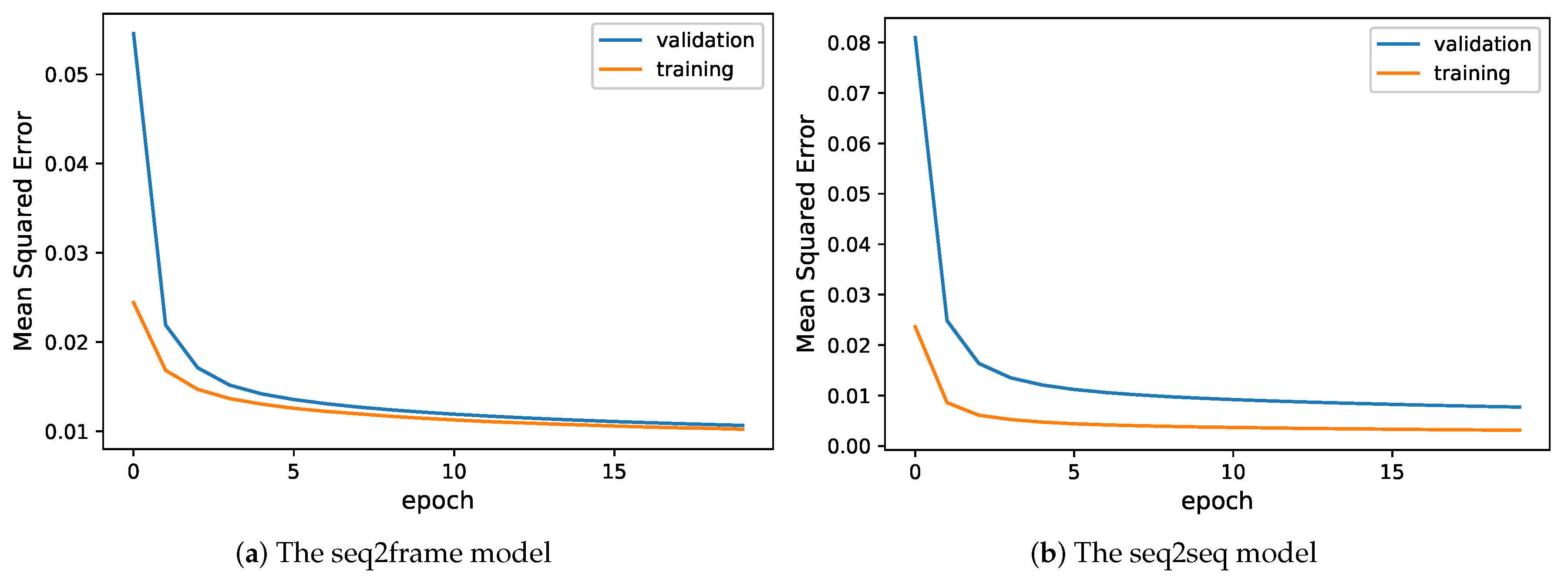
Figure 4a,b reports the training and validation errors under the seq2frame and seq2seq models, respectively. Both models converged in 10 epochs, while the patterns of their convergence are different. Under the seq2frame model, both the training error and validation error drop sharply within the first three epochs, and then the gap between them gradually decreases. By contrast, the gap between the training error and validation error under the seq2seq model remains at a stable level even after 15 epochs. The different error patterns may be due to the different ways of extracting the target variable y under the two models, as shown in Figure 3d,e.

4.4. Visualization of Predictions

To visualize part of the predicted results, Figure 5 shows four s t a t i o n s × f e a t u r e air quality maps randomly selected from the testing dataset, as well as the corresponding predicted station × feature frames by the seq2seq model with l = 24 and Δ t = 48 . For each square of the station × feature matrix, the dark blue color represents a larger value and the light blue color indicates a smaller value.
The far right-end three columns (corresponding to the three meteorological measurements: air pressure, air temperature, and air humidity) of the ground-truth map are almost identical across seven stations. In contrast, the levels of air pollutants recorded by different stations are quite different. For example, the levels of O3 (the third column) reported at different locations show very different patterns, and in the third frame, stations 2 and 5 reported a much higher value than other stations. The proposed model can make an accurate prediction of O3 for each station. We also observe that the values of air pressure in the third frame are much lower than the other three frames, and the level of suspended particulate matter, PM10 and PM2.5, in the last frame is serious, with the level of PM10 from stations 1 and 6 being the top two highest. These trends are all correctly predicted by our proposed seq2seq model. From the visualization results, we conclude that (1) the patterns of the nine air quality measurements are different from one another and (2) the proposed model can make an accurate prediction based on all of the nine measurements from seven stations.
To examine the proposed air quality model across different cities, we conducted another experiment with seven stations from seven major cities in China, including Beijing, Shanghai, Chengdu, Wuhan, Guangzhou, Xi’an, and Nanjing. The data were collected daily (instead of hourly) on seven pollutants (AQI, PM2.5, PM10, SO2, CO, NO2, and O3) from 2 December 2013 to 29 February 2020 for each city. Figure 6 shows that the performance of air quality prediction for seven cities is not as good as that for the seven stations from the same city of Chengdu. One possible reason is that the spatial correlation among seven stations in Chengdu is much stronger than the seven cities that are far away from each other. This is consistent with our general understanding, thus proving the effectiveness of the proposed LS-deGCN in capturing spatial associations.

4.5. Evaluation with Three Metrics

RMSE. As discussed in Section 3.2, the proposed model can predict the future level of air pollution from 1 h to 48 h by varying l from 1 to 48. Moreover, the data used for prediction can be a collection of samples on the last day or the last several days, for which Δ t is used to control the length of samples. In other words, we can vary the parameter Δ t to obtain different training and testing datasets for different experiments. We explore six experiments by combinations of l = { 1 , 24 , 48 } and Δ t = { 24 , 48 } . Therefore, we utilize the data collected from yesterday and the last two days to predict the air quality for one hour later, one day later, and two days later, respectively.
Table 2 displays the RMSEs from the testing set for l = { 1 , 24 , 48 } concerning Δ t = { 24 , 48 } . The RMSEs of the non-stationary LS-deGCN seq2frame and seq2seq models can be calculated directly based on the station × feature matrix. However, for the other three models, we need to conduct training and testing for each pollutant separately, and then calculate the average RMSE over all the pollutants. Our proposed models demonstrate significant improvements compared with the baseline methods and, in particular, the non-stationary LS-deGCN seq2seq model achieves the best performance under all six scenarios. The LSTM-based methods outperform the traditional linear regression and support vector regression. Moreover, the RMSEs of our models increase as the time lag l increases and decreases as Δ t takes a larger value. Intuitively, predicting air quality two days in the future is more challenging than predicting it one hour in the future. However, as the sample size increases, the accuracy of prediction improves, as more historical information can help us capture long-term trends in the data.
Accuracy. Table 3 compares the accuracy of air quality prediction among the five methods for combinations of l = { 1 , 24 , 48 } and Δ t = { 24 , 48 } . The proposed non-stationary LS-deGCN seq2frame and seq2seq models yield much higher accuracy than the others, and the non-stationary LS-deGCN seq2seq model achieves the highest accuracy among all.
MAE. Table 4 shows the MAE of all the methods for the six scenarios with l = { 1 , 24 , 48 } and Δ t = { 24 , 48 } . In those experiments, the two proposed models, the non-stationary LS-deGCN seq2frame and seq2seq models, report much lower MAE than the others, and the non-stationary LS-deGCN seq2seq model outperforms all the rest of the competitors.
For the three metrics, we also observe that the scenarios with Δ t = 48 outperforming those with Δ t = 24 , especially for the LSTM-based methods (i.e., LSTM seq2scalar, non-stationary LS-deGCN seq2frame and seq2seq). This is expected as the prediction of air quality with the historical data of the last two days is a better strategy than that of only utilizing the data of yesterday. Apart from that, models that take into account spatial dependence (Non-stationary LS-deGCN seq2frame and Non-stationary LS-deGCN seq2seq) perform better than models that do not consider spatial dependence (Linear regression, Support vector regression, and LSTM seq2scalar), which demonstrates the necessity and effectiveness of considering spatial correlation.
For the results of RMSE and MAE in Table 2 and Table 4, we observe that the performances continue to decrease when the value of l increases. However, for the accuracy results in Table 3, we observe that the performance does not monotonically decrease with an increasing value of l for our models. In contrast, the accuracy achieves a peak at l = 24 and the performance deteriorates for both l = 1 and l = 48 . This indicates that the three evaluation metrics do not exactly match with each other. As discussed earlier, the larger the time lag l, the more difficult it is to make a prediction. However, if l is too small, the overlapped information under the non-stationary LS-deGCN seq2seq model would be large. The model may not fully capture the dynamic changes in the data, resulting in overly simple weight updates. At the same time, the error information may be concentrated on recent data, making the gradient update too drastic, which affects the model’s prediction performance.

5. Conclusions

In this paper, we train a non-stationary LS-deGCN to fit the spatial–temporal data, a multi-station air pollution dataset of Chengdu from 1 January 2013 to 31 December 2016. On one hand, the de-trending long short-term structure of LS-deGCN can capture the non-stationary temporal dependency between the predicted values and the historical records. On the other hand, the diffusion graph convolution on the station × feature grid gains more power to extract the spatial dependency among stations than a fully connected network. According to the scheme of extracting samples and targets, we propose two sub-models, the non-stationary LS-deGCN seq2frame and non-stationary LS-deGCN seq2seq. The target of the former model is a frame while the latter is a l-shifted sequence. We evaluate both models based on the RMSE, accuracy, and MAE and demonstrate their outstanding performances in comparison with the existing works. However, air quality prediction involves many other factors such as geographical information and traffic information. In future work, we will incorporate other data and integrate them into the framework of the non-stationary LS-deGCN.

Author Contributions

Conceptualization, G.Y. and B.L.; methodology, B.L. and M.H.; software, M.H.; validation, M.H.; formal analysis, B.L. and M.H.; investigation, M.H.; resources, G.Y. and B.L.; data curation, M.H.; writing—original draft preparation, B.L. and M.H.; writing—review and editing, G.Y.; visualization, M.H.; supervision, G.Y. and B.L.; project administration, G.Y. and B.L.; funding acquisition, G.Y. All authors have read and agreed to the published version of the manuscript.

Funding

The research of Guosheng Yin was partially supported by the Theme-based Research Scheme (TRS) from the Research Grants Council of Hong Kong, Institute of Medical Intelligence and XR (T45-401/22-N).

Institutional Review Board Statement

Not applicable.

Informed Consent Statement

Not applicable.

Data Availability Statement

The data are not publicly available due to privacy.

Acknowledgments

We thank the editors and reviewers for their helpful suggestions.

Conflicts of Interest

The authors declare no conflicts of interest.

Abbreviations

AQIAir quality index
CNNConvolutional neural network
GCNGraph convolution network
GNNGraph neural network
LSTMLong short–term memory
LS-deGCNLong–short de-trending graph convolutional network
NLPNatural language processing
RNNRecurrent neural network
RMSERoot mean squared error
MAEMean absolute error

References

  1. Janarthanan, R.; Partheeban, P.; Somasundaram, K.; Elamparithi, P.N. A deep learning approach for prediction of air quality index in a metropolitan city. Sustain. Cities Soc. 2021, 67, 102720. [Google Scholar] [CrossRef]
  2. Singh, V.; Carnevale, C.; Finzi, G.; Pisoni, E.; Volta, M. A cokriging based approach to reconstruct air pollution maps, processing measurement station concentrations and deterministic model simulations. Environ. Model. Softw. 2011, 26, 778–786. [Google Scholar] [CrossRef]
  3. Ayturan, Y.A.; Ayturan, Z.C.; Altun, H.O. Air pollution modelling with deep learning: A review. Int. J. Environ. Pollut. Environ. Model. 2018, 1, 58–62. [Google Scholar]
  4. Zhang, S.; Guo, B.; Dong, A.; He, J.; Xu, Z.; Chen, S.X. Cautionary tales on air-quality improvement in Beijing. Proc. R. Soc. A Math. Phys. Eng. Sci. 2017, 473, 20170457. [Google Scholar] [CrossRef] [PubMed]
  5. Qi, Z.; Wang, T.; Song, G.; Hu, W.; Li, X.; Zhang, Z. Deep air learning: Interpolation, prediction, and feature analysis of fine-grained air quality. IEEE Trans. Knowl. Data Eng. 2018, 30, 2285–2297. [Google Scholar] [CrossRef]
  6. Bessagnet, B.; Beauchamp, M.; Menut, L.; Fablet, R.; Pisoni, E.; Thunis, P. Deep learning techniques applied to super-resolution chemistry transport modeling for operational uses. Environ. Res. Commun. 2021, 3, 085001. [Google Scholar] [CrossRef]
  7. Zhu, J.Y.; Sun, C.; Li, V.O. Granger causality based air quality estimation with spatio-temporal (ST) heterogeneous big data. In Proceedings of the 2015 IEEE Conference on Computer Communications Workshops (INFOCOM WKSHPS), Hong Kong, China, 26 April–1 May 2015; pp. 612–617. [Google Scholar]
  8. Zhu, J.Y.; Sun, C.; Li, V.O. An extended spatio-temporal Granger causality model for air quality estimation with heterogeneous urban big data. IEEE Trans. Big Data 2017, 3, 307–319. [Google Scholar] [CrossRef]
  9. Huang, C.J.; Kuo, P.H. A deep CNN-LSTM model for particulate matter (PM2.5) forecasting in smart cities. Sensors 2018, 18, 2220. [Google Scholar] [CrossRef]
  10. Li, X.; Peng, L.; Yao, X.; Cui, S.; Hu, Y.; You, C.; Chi, T. Long short-term memory neural network for air pollutant concentration predictions: Method development and evaluation. Environ. Pollut. 2017, 231, 997–1004. [Google Scholar] [CrossRef]
  11. Fan, J.; Li, Q.; Hou, J.; Feng, X.; Karimian, H.; Lin, S. A spatiotemporal prediction framework for air pollution based on deep RNN. ISPRS Ann. Photogramm. Remote Sens. Spat. Inf. Sci. 2017, 4, 15–22. [Google Scholar] [CrossRef]
  12. Wang, J.; Song, G. A deep spatial-temporal ensemble model for air quality prediction. Neurocomputing 2018, 314, 198–206. [Google Scholar] [CrossRef]
  13. Shi, X.; Zhourong, C.; Hao, W.; Yeung, D.; Wong, W.; Woo, W. Convolutional LSTM network: A machine learning approach for precipitation nowcasting. In Proceedings of the Advances in Neural Information Processing Systems, Montreal, QU, Canada, 11–12 December 2015; pp. 802–810. [Google Scholar]
  14. Li, Y.; Yu, R.; Shahabi, C.; Liu, Y. Diffusion Convolutional Recurrent Neural Network: Data-Driven Traffic Forecasting. In Proceedings of the International Conference on Learning Representations (ICLR ’18), Vancouver, BC, Canada, 30 April–3 May 2018. [Google Scholar]
  15. Deodatis, G. Non-stationary stochastic vector processes: Seismic ground motion applications. Probabilistic Eng. Mech. 1996, 11, 149–167. [Google Scholar] [CrossRef]
  16. Wang, Y.; Zhang, J.; Zhu, H.; Long, M.; Wang, J.; Yu, P.S. Memory In Memory: A predictive neural network for learning higher-order nonstationarity from Spatio-temporal dynamics. In Proceedings of the IEEE Conference on Computer Vision and Pattern Recognition, Long Beach, CA, USA, 15–20 June 2019; pp. 9154–9162. [Google Scholar]
  17. Liu, B.; Yan, S.; Li, J.; Li, Y. Forecasting PM2.5 concentration using spatio-temporal extreme learning machine. In Proceedings of the 2016 15th IEEE International Conference on Machine Learning and Applications (ICMLA), Anaheim, CA, USA, 18–20 December 2016; pp. 950–953. [Google Scholar]
  18. Ghaemi, Z.; Alimohammadi, A.; Farnaghi, M. LaSVM-based big data learning system for dynamic prediction of air pollution in Tehran. Environ. Monit. Assess. 2018, 190, 300. [Google Scholar] [CrossRef] [PubMed]
  19. Liu, B.C.; Binaykia, A.; Chang, P.C.; Tiwari, M.K.; Tsao, C.C. Urban air quality forecasting based on multi-dimensional collaborative support vector regression (svr): A case study of Beijing-Tianjin-Shijiazhuang. PLoS ONE 2017, 12, e0179763. [Google Scholar] [CrossRef] [PubMed]
  20. Mukhopadhyay, S.; Sahu, S.K. A Bayesian spatiotemporal model to estimate long-term exposure to outdoor air pollution at coarser administrative geographies in England and Wales. J. R. Stat. Soc. Ser. A 2018, 181, 465–486. [Google Scholar] [CrossRef]
  21. Lotrecchiano, N.; Sofia, D.; Giuliano, A.; Barletta, D.; Poletto, M. Pollution dispersion from a fire using a Gaussian plume model. Int. J. Saf. Secur. Eng 2020, 10, 431–439. [Google Scholar] [CrossRef]
  22. Russo, A.; Raischel, F.; Lind, P.G. Air quality prediction using optimal neural networks with stochastic variables. Atmos. Environ. 2013, 79, 822–830. [Google Scholar] [CrossRef]
  23. Biancofiore, F.; Busilacchio, M.; Verdecchia, M.; Tomassetti, B.; Aruffo, E.; Bianco, S.; Di Tommaso, S.; Colangeli, C.; Rosatelli, G.; Di Carlo, P. Recursive neural network model for analysis and forecast of PM10 and PM2.5. Atmos. Pollut. Res. 2017, 8, 652–659. [Google Scholar] [CrossRef]
  24. Kök, İ.; Şimşek, M.U.; Özdemir, S. A deep learning model for air quality prediction in smart cities. In Proceedings of the IEEE International Conference on Big Data (Big Data), Boston, MA, USA, 11–14 December 2017; pp. 1983–1990. [Google Scholar]
  25. Hochreiter, S.; Schmidhuber, J. Long short-term memory. Neural Comput. 1997, 9, 1735–1780. [Google Scholar] [CrossRef]
  26. Sutskever, I.; Vinyals, O.; Le, Q.V. Sequence to sequence learning with neural networks. In Proceedings of the Advances in Neural Information Processing Systems, Montreal, QU, Canada, 12–14 December 2014; pp. 3104–3112. [Google Scholar]
  27. Srivastava, N.; Mansimov, E.; Salakhudinov, R. Unsupervised learning of video representations using LSTMs. In Proceedings of the International Conference on Machine Learning, Lille, France, 6 –11 July 2015; pp. 43–852. [Google Scholar]
  28. Guo, T.; Lin, T.; Lu, Y. An interpretable LSTM neural network for autoregressive exogenous model. In Proceedings of the Workshop of International Conference on Learning Representations, Vancouver, BC, Canada, 30 April–3 May 2018. [Google Scholar]
  29. Xu, J.; Liu, X.; Wilson, T.; Tan, P.N.; Hatami, P.; Luo, L. MUSCAT: Multi-scale spatio-temporal learning with application to climate modeling. In Proceedings of the International Joint Conference on Artificial Intelligence, Stockholm, Sweden, 13–19 July 2018; pp. 2912–2918. [Google Scholar]
  30. Shuman, D.I.; Narang, S.K.; Frossard, P.; Ortega, A.; Vandergheynst, P. The emerging field of signal processing on graphs: Extending high-dimensional data analysis to networks and other irregular domains. IEEE Signal Process. Mag. 2013, 30, 83–98. [Google Scholar] [CrossRef]
  31. Wilson, T.; Tan, P.N.; Luo, L. A low rank weighted graph convolutional approach to weather prediction. In Proceedings of the IEEE International Conference on Data Mining, Singapore, 17–20 November 2018; pp. 627–636. [Google Scholar]
  32. Burden, R.L. Numerical Analysis; Brooks/Cole Cengage Learning: Belmont, CA, USA, 2011. [Google Scholar]
  33. Akanbi, L.A.; Oyedele, A.O.; Oyedele, L.O.; Salami, R.O. Deep learning model for Demolition Waste Prediction in a circular economy. J. Clean. Prod. 2020, 274, 122843. [Google Scholar] [CrossRef]
Figure 1. A sketch of non-stationary records of the features of temperature, pressure, PM2.5, and O3.
Sustainability 16 00165 g001
Figure 2. There are nine stations spatially distributed in Chengdu city, and CO and PM2.5 levels at stations 4 and 5 are recorded on an hourly basis. (a) Nine monitoring stations in the city of Chengdu. (b) Spatial graph G = ( V , E , A ) . V, E, and A denote the vertex set, edge set, and adjacent matrix of the graph, respectively. (c) The records of levels of CO and PM2.5 from station 4 and station 5 over one week. From panel (a), we observe a long geographic distance between stations 4 and 5 and a strong correlation between the CO and PM2.5 readings at these two stations in panel (c). Spatial correlation: stations 3 and 9 have the same readings, so 9 is removed. We also removed station 8 because 40% of the data was missing. Panel (b) illustrates the spatial dependency graph among the seven stations we studied.
Sustainability 16 00165 g002
Figure 3. Overview of the proposed model framework. (a) Depicts the original spatial graph among the seven stations constructed based on their geographical distance; (b) illustrates the process of diffusion graph convolution, which takes the geographical graph as input and outputs a refined graph; (c) demonstrates the de-trending process; (d) displays prediction using the seq2frame mode; and (e) presents prediction using the seq2seq mode.
Sustainability 16 00165 g003
Figure 4. Mean squared errors for the training and validation datasets under (a) the seq2frame model, and (b) the seq2seq model, with the time lag l = 48 and the window width Δ t = 48 .
Sustainability 16 00165 g004
Figure 5. Visualization of the four ground-truth station × feature frames randomly selected from the testing dataset (right panel) and the corresponding prediction (left panel) by the seq2seq model with time lag l = 24 and Δ t = 48 . The color transition from light blue to dark blue corresponds to an increase in value from small to large, with all values normalized to the range [0, 1].
Sustainability 16 00165 g005
Figure 6. Visualization of the four ground-truth station × feature frames randomly selected from the testing dataset (right panel) and the corresponding prediction (left panel) by the seq2seq model for seven major cities in China. The color transition from light blue to dark blue corresponds to an increase in value from small to large, with all values normalized to the range [0, 1].
Sustainability 16 00165 g006
Table 1. Partition for training, validation, and testing datasets.
DatasetsDescription
TrainingData from 1 January 2013 to 31 December 2015
ValidationData from 1 January 2016 to 1 June 2016
TestingThe remaining data
Table 2. Comparison of the root mean squared error (RMSE) among different methods based on the Chengdu testing dataset, where a smaller RMSE indicates a better result.
Models l = 1 l = 24 l = 48
Linear regression1.781.822.23
Support vector regression1.611.931..98
Δ t = 24LSTM seq2scalar1.041.121.25
Non-stationary LS-deGCN seq2frame0.580.781.1
Non-stationary LS-deGCN seq2seq0.560.770.87
Linear regression1.671.792.03
Support vector regression1.521.761.95
Δ t = 48LSTM seq2scalar0.870.920.95
Non-stationary LS-deGCN seq2frame0.450.620.67
Non-stationary LS-deGCN seq2seq0.390.560.57
Table 3. Comparison of accuracy among different methods based on the Chengdu testing dataset, where a higher value of accuracy indicates a better result.
Models l = 1 l = 24 l = 48
Linear regression0.56340.53670.5278
Support vector regression0.57630.55980.5557
Δ t = 24LSTM seq2scalar0.70210.71670.7198
Non-stationary LS-deGCN seq2frame0.72340.75450.7517
Non-stationary LS-deGCN seq2seq0.73650.76520.7482
Linear regression0.56120.54230.5186
Support vector regression0.58340.56540.5521
Δ t = 48LSTM seq2scalar0.68250.72120.7237
Non-stationary LS-deGCN seq2frame0.72350.78660.7655
Non-stationary LS-deGCN seq2seq0.76550.81230.7785
Table 4. Comparison of the mean absolute error (MAE) among different methods based on the Chengdu testing dataset, where a smaller MAE indicates a better result.
Models l = 1 l = 24 l = 48
Linear regression0.01750.02110.0234
Support vector regression0.01580.01470.0186
Δ t = 24LSTM seq2scalar0.01480.01670.0166
Non-stationary LS-deGCN seq2frame0.00920.00910.0101
Non-stationary LS-deGCN seq2seq0.00770.00890.0093
Linear regression0.01780.01980.0211
Support vector regression0.01530.01320.0201
Δ t = 48LSTM seq2scalar0.01360.01420.0154
Non-stationary LS-deGCN seq2frame0.00800.00790.0091
Non-stationary LS-deGCN seq2seq0.00710.00780.0083
Disclaimer/Publisher’s Note: The statements, opinions and data contained in all publications are solely those of the individual author(s) and contributor(s) and not of MDPI and/or the editor(s). MDPI and/or the editor(s) disclaim responsibility for any injury to people or property resulting from any ideas, methods, instructions or products referred to in the content.

