Intra-Household Income Management and Couple’s Relative Sharing of Income and Environment Sustainability in Japan

Abstract

This study aims to identify household members’ income sharing, when the amount of said income is governed by a particular household member. The results are expected to provide insightful evidence that identifies who is under the poverty line within families. This will illustrate the intra-household allocation inequality by observing the members’ household income dominance. Using the information on household income management obtained from the Japanese Household Panel Survey data (1993–2013) and the original Internet survey, this paper develops an alternative methodology to estimate the household income distribution of couples. A two-step estimation process was employed to estimate the wife’s manageable income equation. Then, the parameters were substituted into the husband’s manageable income equation to estimate the parameters for calculating the wife’s sharing rule. The results are as follows. First, a wife’s share of intra-household resources positively correlates to her manageable income resources. However, wives have weak power in expending the transferred income from their husbands. Second, the remarkable feature is that, on average, wives share 37% of the resources, meaning that the wives’ relative bargaining is weaker than the husbands’. Narrowing the gap in terms of hourly wage between husbands and wives is a crucial tool to reduce the intra-household allocation gap. Third, the wives’ relative intrahousehold income allocation improvement is associated with household environment sustainability activities. To improve the intra-household income allocation inequality, we provide an original approach to explore the intra-household head of household members’ relative income sharing. The results highlight the inequality of intra-household income distribution and confirm that reducing the income gap would be a crucial improvement factor.

1. Introduction

In 2015, the United Nations proposed the 17 sustainable development goals (SDGs) to enhance humanity’s well-being (UN 2015). For instance, the fifth goal highlights taking action to empower women and girls and ensure their equal rights. Additionally, the tenth goal presents the reduced inequalities. Moreover, in order to sustain the natural environment, the 13th goal of the SDGs is climate action, indicating that human beings should take action immediately to stop global warming as worldwide carbon dioxide emission has increased by around 50% since 1990. This study aims to identify the intra-household income allocation sharing rule between wives and husbands to confirm whether there is income allocation inequality and the determinants of the disparity. Furthermore, the relationship between inequality and household environment sustainability activities is explored to contribute to the United Nations’ sustainable development goals.

The exploration of household members’ relative sharing of household income is adopted to measure the intra-household income allocation equality; that is, the relative amount of income governed by a particular household member has gained increased interest among researchers [1,2,3,4]. This research is primarily used to explore the intra-household resource allocation gap. However, the methods typically rely on the utility function of consumption and time use, which leads to difficulties in controlling the preference heterogeneity among wives or husbands caused by the complex structure model. In the traditional methodology, in order to identify the wife’s sharing rule (relative sharing of resources), traditional methodology generally uses the utility function to derive the demand function, which is to proxy the preference. On the other hand, the sharing rule function is a function of determinant factors of the sharing rule. Additionally, the wife’s and husband’s demand functions are then estimated with the sharing rule function. This traditional methodology makes it difficult to control a number of preference heterogeneities. Therefore, we generally assume that the wives or the husbands have the same (or a similar) preference for private consumption and leisure. In order to address the limitations, this paper proposes an alternative method that can estimate the relative sharing of resources without using the utility function. One of the remarkable contributions in investigating whether wives or husbands have the same preference is matter.

The unitary model, which assumes traditional household decision-making, assumes that each household has a single agent who maximizes the utility function based on the household’s budget constraints or that multiple agents behave as a single unit given the same utility function and budget constraints. This household consumption model is based on the income pooling hypothesis, and the test of the reality of the unitary model is improved. Income pooling indicates that an individual’s income does not impact household consumption behavior unless the total amount of income is changed. Empirical studies test this hypothesis and conclude weak support for the unitary model [2,5,6,7].

Theoretically, the collective model, which improves the unitary model, is proposed by Chiappori [1] and allows for researchers to explore the relationship between household members’ expenditures and their preference heterogeneity, and is becoming popular. The collective model describes household-level decisions by maximizing the aggregate household utility, which is the weighted sum of a member’s utility. The relative bargaining power of the members comprises the weights. The members’ relative bargaining powers are assumed to be determined by their relative income, relative age, and other characteristics (e.g., divorce ratio).

Numerous studies have been conducted based on the collective model [2,3,4,8,9,10,11,12]. For example, the results of these studies uncover the individual levels of resource sharing [10], making poverty observable at the individual level rather than at the household level. Couprie [9] conducted a study based on the collective model using British households and found that women have fewer private expenditures than their husbands, which highly relies on the gender wage gap. To reduce the intra-household resource-sharing gap, decreasing the gender wage gap is a tool. Lise and Yamada [11] utilize Japanese household data to investigate intra-household income allocation; they find that even when the wives and husbands have the same wage, the wives tend to spend around half as much of the private expenditure than their husbands do.

As an investigation of the intra-household resource allocation associated with enhancing the family member well-being, empirically, the intra-household income allocation within the family members has been widely investigated in previous studies [13,14,15,16,17,18,19,20,21,22,23,24,25,26,27,28,29,30,31,32]. Xu [31] used household data to show the intra-household allocation of educational resources within Bangladesh households. Similarly, Lechene [32] provided an alternative estimation methodology to identify the intra-household income allocation among family members; they used the 12-country household data to show that the equivalent income distribution hypothesis is rejected, and a large gender gap still exists in many countries. Regarding household pro-environmental behavior, more natural environmental conservation behavior is required, and the natural environment has worsened rapidly in recent years [33,34,35]. If gender has an influence on the different preferences regarding environment conservation attitudes or the intra-household income, inequality may reduce the low bargaining power of family members’ environment conservation activities, and the improvement of the intra-household income inequality may lead the household members being more likely to protect the natural environment.

The proceeding studies utilized the household consumption information derived from the wives and husbands associated with bargaining power. The intra-household sharing rule function is estimated in the structure form. However, measurement errors may exist in the survey, and the results may be biased in estimating household members’ bargaining power if the members’ consumption information contains a measurement error. In order to address the issue or to confirm the robust results of the sharing rule of the household income allocation, we developed an alternative way to estimate the household income allocation using household income management information. Consistent with the previous studies, we aim to explore the relationship between intra-household income allocation and identify whether household income is distributed equally to wives and husbands. Aside from the consumption measurement issue, as the natural environment worsens rapidly, households are required to contribute to environment conservation. However, investigations of household environment conservation activities and intra-household income allocation are scarce. This study aims to fill this knowledge gap. The relationship between the wives’ involvement in natural environment conservation and intra-household income inequality is investigated.

The contribution of this study to the current literature is summarized in the following two points. First, based on the collective model, this study adopts an original method for exploring the leading intra-household members’ relative sharing of resources (or income) using the Japanese Household Panel Survey (JHPS) data. Unlike most previous research studies, this study utilized information about intra-household income transfer between couples, which allowed for an observation of the leading adults’ management of household income. This study firstly estimates the intra-household wives’ and husbands’ sharing rule income allocation based on their management of household income in Japan.

Secondly, the exogenous characteristics influencing household income allocation, including wives’ wages, husbands’ wages, household non-labor income, social divorce ratio, and social gender ratio, are adopted. Furthermore, the impact of each bargaining power characteristic on the intra-household income allocation is examined to provide the policy implications in order to improve the inequality within the households. Third, the relationship between household income allocation inequality and the wives’ environment conservation activities is investigated. The resulting objective is to sustain society by reducing intra-household income allocation inequality and the households’ environment conservation attitudes to achieve the United Nations’ sustainable development goals. The results may provide insightful evidence of the households’ relationship with sustainability to the policy-makers.

This study is structured as follows. Section 2 describes the theory and estimation model. Section 3 explains the data. Section 4 shows the specification. Finally, Section 5 draws estimation results and implications. Finally, Section 6 provides the discussion and policy implication of this study.

2. Model

The theoretical framework follows studies by Chiappori [1] and Browning et al. [2] with households with two family members (h for husband, w for wife). Each member has his or her specific preference and makes Pareto-efficient decisions. This model assumes that private goods are weakly separable from public goods. Private goods are divided into categories. The model showed that two-member households maximize the weighted utility function ($U^w\left(x^w,Q\right))$ with private consumption $x^w$ and public goods $Q$; and $U^h\left(x^h,Q\right))$ with private consumption $x^h$ and public goods subject to the budget constraints. Therefore, the household consumption decision is described as follows:

$$\begin{gathered} {\mathrm{m}\mathrm{a}\mathrm{x}}_{x^w,x^y,Q }\mu (y^w,y^h,\mathit{L}){\mathbf{U}}^{\mathbf{w}}(x^w,Q)+(1-\mu (y^w,y^h,\mathit{L})){\mathbf{U}}^{\mathbf{h}}(x^h,Q) \\ \begin{array}{l}\mathrm{Subject}\mathrm{to}\hfill \end{array} \\ \sum _j^n{x}^w+\sum _j^n{x}^y+Q=y^w+y^h, \end{gathered}$$

(1)

where $\mu \left(y^w,y^h,\mathit{L}\right)\in$ (0, 1) is a continuous function for the “distribution power.” A value close to 1 means that the household member has a strong distribution power, and a value close to 0 means that the household member has a weak distribution power. There is a function of the wife’s income $y^w$, of the husband’s income $y^h$, and the other factors are represented by L.

3. Data

The Japanese Panel Survey of Consumers (JPSC), improved by the Institute for Research on Household Economics, was used in this study. The JPSC data survey is conducted annually and includes detailed demographic, income management, income, savings, and expenditures information from young-aged households. The first cohort (Cohort A) was recruited in 1993, and new cohorts have been added every five years since then (Cohort B in 1998, Cohort C in 2003, Cohort D in 2008, etc.). Cohort A included randomly recruited young women ages 24–34. Other cohorts included young women ages 24–29. The men’s information was collected from the husbands of the recruited married women. Therefore, there are no data for single men. When these data were collected, the questionnaire item regarding income management asked the young women to specify how much money their husbands transfer them or how much they transfer to their husbands. Money transfer indicates an entrustment of the management of that income.

3.1. Definition of Resource Management

Two resource management situations are displayed in

Table 1. Resource management situations and examples.

	Resource Management Situation	Example
Case 1.	The resource belongs to only one household member	(1) Leisure time
		(2) Housework time
		(3) Non-transferred income
Case 2.	Resource manageable to wife and husband	(1) Wife transfers her income to husband
		(2) Husband transfers his income to wife

Note: Created by authors.

. The situations are resources belonging to the only household member (wife or husband) and resources belonging to both the husband and wife. Case 1 resources include leisure time, housework time, and non-transferred income; the household member cannot determine how much leisure time the other Fmember spends. The resources managed by couples (Case 2) through income transfer include two situations: The husband transfers income to the wife, or the wife transfers income to the husband. If a households exist wherein the husband transfers to the wife and the wife transfers to the husband, the husband and wife manage more resources.

3.2. Definition of Intra-Household Resource Management

The measure of intrahousehold income transfer is a key variable in this study. The questionnaire item regarding income management asks the young women to specify how much money their husbands transferred to them or they transferred to their husbands in September. Money transfers indicate entrustment with the management of that income.

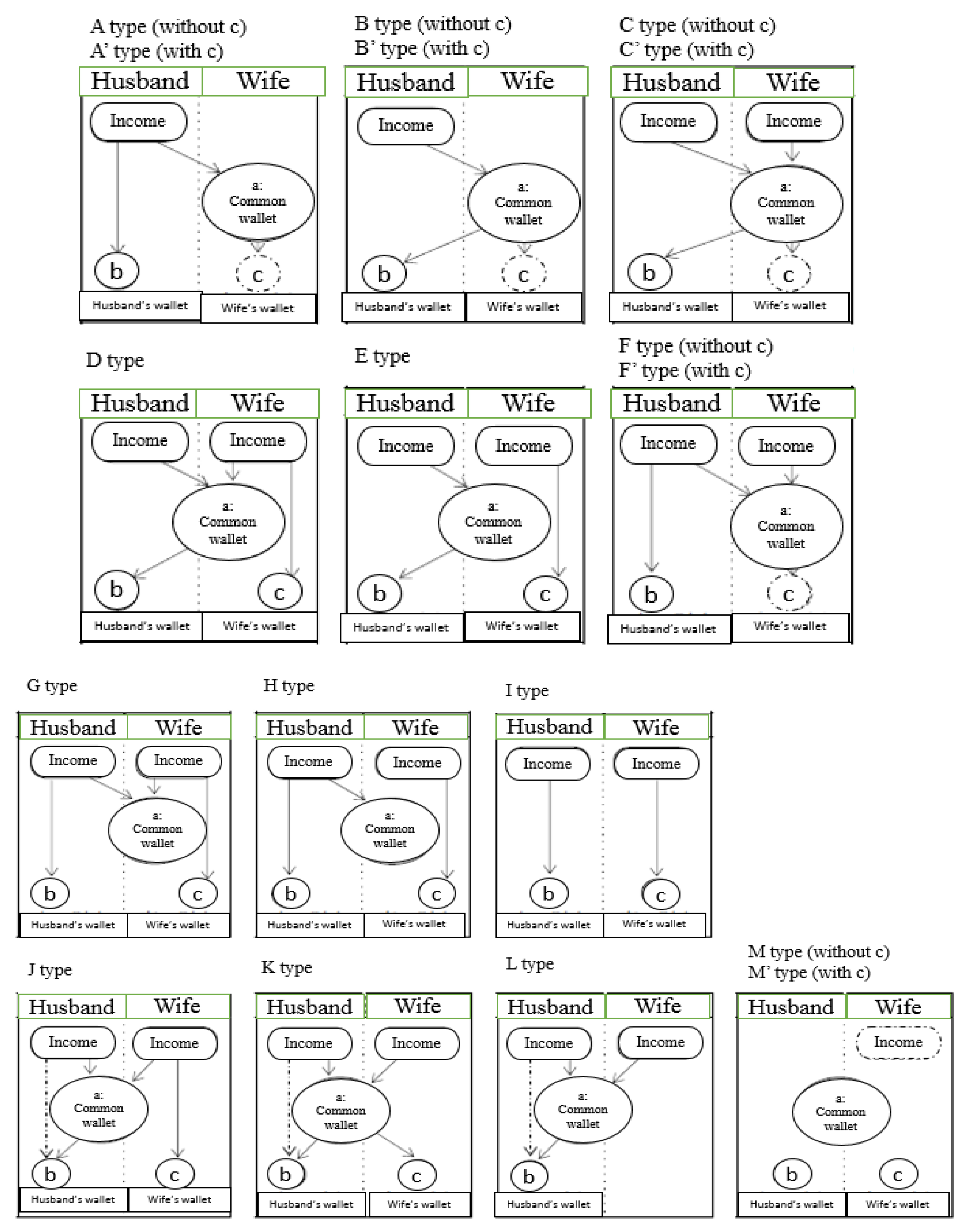
Intra-household income management types A–M′ are displayed in Figure 1, and the exact figure in the questionnaire was translated by the author. Types A and A′ indicate that only the husband works and transfers part of his income to the spouse, who does not have an income. Types B and B′ indicate that only the husband works, transfers all of his income to the spouse, who does not have an income, and then receives pocket money from the wife. Types C and C′ indicate that the husband transfers all of his income to his spouse, who also has an income, who then gives him pocket money and pools all of her income in the shared wallet. Type D indicates that the husband transfers all of his income to the spouse and then receives pocket money from the spouse, who pools part of her income in the common wallet. Type E indicates that the husband transfers all his income and receives pocket money from the spouse, who does not pool her income in the common wallet.

Types F, F′, G, and H indicate the husbands transfer part of his income to the spouse, and in types F and F′, the wife pools all of her income in the common wallet. In Type G, the wife pools part of her income in the common wallet, while in Type H, the wife does not pool her income in the common wallet. Type I indicates that the couple does not transfer income to each other. Type J indicates that the wife transfers part of her income to the spouse. Type K indicates that the wife transfers all of her income to the spouse and then receives pocket money from the husband. Type L indicates that the wife transfers all of her income to the husband and does not receive any pocket money. Type M indicates that neither the husband nor the wife have income (in the month studied, September). Type M′ indicates that only the wife has income. The difference between types A, B, C, and F and types A′, B′, C′, and F′ is that the wife has pocket money in the latter but not the former.

The commonly managed resource defined in this study is the amount of income transferred by the wife or the husband to the other. It is worth noting that the amount of the commonly managed resource is not the same as the common wallet because the husband may not manage the common wallet after transferring his income to the spouse (e.g., Type C). Based on the income management types, the intra-household income transfer can be categorized as in

Table 2. Intra-household income transfer and income management type.

Intra-Household Income Transfer	Income Management Type (See Figure 1)
Wife’s transfer of income to spouse	Transferred part of her income: Type J
	Transferred all her income: Type K, L
Husband’s transfer of income to spouse	Transferred part of his income: Type F, F′, G, H
	Transferred all his income: Type C, C′, D, E
No intra-household income transfer	Type I

Note: In our sample, both husband and wife work, so income management Type A, A′, B, B′, M, and M′ are not included.

. There are three scenarios of income transfer among couples with both members working: the wife transfers her income to the spouse (Type J for part of the wife’s income and types K and L for all of her income), the husband transfers his income to the spouse (types F, F′, G, and H for part of the husband’s income and types C, C′, D, and E for all of his income), and there is no income transfer (Type I). For the transferred amount, we use the reported amount if the spouses transfer part of their income and the amount of the reported September disposable income if the spouses transfer all of their income. In the case when one spouse transfers all their income to the other, who dispenses pocket money, we select the individuals’ total disposable income as the transferred income amount because the spouses can influence the amount of pocket money.

The main variables are described in

Table 3. Variable descriptions.

Variable	Description
Hourly wage
Wife’s hourly wage	Wife’s hourly wage if the wife reported an hourly wage (JPY)
	Wife’s September disposable income/(4.29 week × weekly working hour) (JPY)
Husband’s hourly wage	Husband’s September disposable income/(4.29 week × weekly working hour) (JPY)
Full income
Wife’s full income (or resource)	Wife’s hourly wage × 24 h (JPY/day)
Husband’s full income (or resource)	Husband’s hourly wage × 24 h (JPY/day)
Household full income	Wife’s full income + husband’s full income (JPY/day)
Intra-household income transfer
Wife’s transfer of income to spouse	September income transfer amount/30 day (JPY/day)
Husband’s transfer of income to spouse	September income transfer amount/30 day (JPY/day)
Resource management
Wife’s relative manageable resource	(Wife’s full income + husband’s transfer of income to spouse)/Household full income
Husband’s relative manageable resource	(Husband’s full-income + wife’s transfer of income to spouse)/Household full income

Note: Created by authors.

. The wife’s hourly wage is reported in two ways. First is the wife’s hourly wage, if reported. Second, as shown in Table 3, the September disposable income is divided by the number of weeks and weekly work hours. The husband’s hourly wage is calculated by dividing his September disposable income by the number of weeks and weekly work hours. In order to calculate the hourly wage in the analysis, the weekly hours are set at 40 h for working men due to the many missing values in the reported weekly hours and the full-time employment status of most husbands in Japan.

The full income (or resources) is the daily full amount of resources, as defined in Table 3. Household full income is the sum of the wife’s full income and the husband’s full income. Household non-labor income in Japan is small, with an annual average JPY 139,000, which means that a household, on average, earns around JPY 380 in non-labor income per day. We, therefore, do not take this amount into account.

The amount of intra-household income transfer is transformed into daily transfers, as shown in Table 3. Again, the household income is either transferred from the wife to the husband or vice versa. If both directions of transfers are reported in the household, we take the maximum amount of income transfer as the commonly managed resource. For example, in Type C (see Figure 1), the husband transfers all of his income to the spouse and then receives pocket money from the wife, who pools all of her income into the common wallet. In his case, the commonly managed resource is the husband’s disposable money, not the sum of the husband’s disposable income and the pocket money or the amount of money in the common wallet. Finally, the wife’s relative managed resources and husband’s relative managed resources are defined at the bottom of Table 3. The detailed descriptive statistics are displayed in

Table 4. Sample statistics.

	Mean	Std. Dev.
Husband’s relative manageable income ($G^h$)	0.642	0.108
Wife’s relative manageable full income ($G^w$)	0.496	0.093
Wife’s hourly wage (JPY)	943.939	450.545
Husband’s hourly wage (JPY)	1692.853	776.687
Household non-labor income (million JPY)	0.139	0.929
Gender ratio (%) (men population/women population)	95.320	0.510
Divorce ratio (%) (current divorce number/marriage number)	34.314	3.651
Observations	9785
Number of households	1736

Note: The sample is from the JPSC 1993–2013 cohorts. The divorce ratio is from the Ministry of Health, Labor, and Welfare [36]. The gender ratio is from the Ministry of Internal Affairs and Communications Statistics Bureau [37].

.

For each cohort, married couples, in which both the husband and the wife were working (either full-time or part-time), and regardless of whether they had children, were selected as the sample. Observations with missing values were excluded. Observations which reported zero income transfers were excluded (around 4%). If the income transfer is zero, the share of resources becomes the full income. Table 1 shows the statistics from the sample. On average, a husband’s relative manageable full income represents 64.2%. On the other hand, the wife’s relative manageable full income represents, on average, 49.6%.

The original Internet survey in Japan was conducted through a third company with an extensive panel, allowing for the collected samples to match the population age, gender, and region from 30 January 2023 to 8 February 2023. The survey is for the Japanese households’ environment conservation attitudes, energy sustainability attitudes, renewable energy usage, willingness to pay for renewable energy, nuclear power energy attitudes and demographic characteristics, and socio-economic background. The relationship between the wives’ environment conservation activities and the intrahousehold income allocation is shown based on this original survey.

A two-step random sampling method is adopted in the original survey. Each cell and targeted sample are determined to match the population age, gender, and perfectional region. In the second step, the respondents are randomly selected to match the population characteristics. When old-age Internet users are scarce, the closed-age respondents are selected to avoid the sample selection bias. Moreover, the questionnaire is double-checked with professionals to remove misleading items from the respondents. Finally, the exclusion items “do not know” or “refuse to answer” are adopted to avoid the missing value. In total, 923 valid married and aged 25 to 55 women observations were collected from 47 prefectures in Japan.

A set of dummy variables are adopted to measure the household’s environment conservation activities. The dummy variable recycling and waste separation and reduction are equal to 1 if the wife is involved; otherwise, it is equal to 0. The variables are as follows: cleanup and trash pickup in respondents’ immediate community; energy-saving actions such as saving electricity and fuel; use of public transportation and bicycles; purchase of recycled products; purchase of energy-saving products; use of renewable energy; purchase of electric vehicles; government-related environmental activities; corporate environmental activities (CSR); environmental activities related to international organizations; environmental education activities; animal protection activities; forest conservation (afforestation, illegal logging control); environmental policy-related activities; environment-related rallies and protests. The other selected control variables that may affect the wife’s involvement in environmental conservation activities are age, education attainment, number of family members, the “having children” dummy, and household income. The interested independent variable is the ratio of the wife’s income to household income measured by her yearly income earned in the last year over her household income.

4. Specification

In order to investigate the intra-household sharing rule between wives and husbands, the specification based on the theoretical framework developed in the section following the Collective model is applied [1]. The theoretical framework follows studies by Chiappori [1] and Browning [2] with a household of two family members (h for husband, w for wife).

The collective model, proposed by Chiappori [1], examines the allocation of the household’s full income (the wife or husband’s full income is their daily wages evaluated every 24 h. The non-working wife and husband are excluded in this study because the hourly wage cannot be calculated directly from the data and the non-working wives’ wages must be estimated. This may cause sample selection bias, but, for example, Chiappori [8] took a similar approach. Alternatively, other research papers include non-working individuals using a different methodology, such as [38] ($Y$), or resources, between husband and wife, $Y=I^w+I^h$, where $I^w$ represents the wife’s full income and $I^h\mathrm{r}\mathrm{e}\mathrm{p}\mathrm{r}\mathrm{e}\mathrm{s}\mathrm{e}\mathrm{n}\mathrm{t}\mathrm{s}\mathrm{t}\mathrm{h}\mathrm{e}$ husband’s full income. The model describes a household maximizing the weighted summation of the wife and husband’s utility under the Pareto efficient assumption. The weight is also known as the Pareto weight or relative bargaining power. Due to the fact that the bargaining is unobservable, monetary-based sharing rules are widely used (see [4] for detailed proof and an explanation). For the equivalent of this model, a household’s decision-making process has two steps: dividing income $Y$ into $Y^w\mathrm{a}\mathrm{n}\mathrm{d} Y^h$ and the wife and husband maximizing the utility separately under $Y^w\mathrm{a}\mathrm{n}\mathrm{d} Y^h$, respectively. The wife’s shared resource is then $Y^w$ and the relative sharing of resources (also known as the sharing rule) is $s^w$, which is defined as $s^w\equiv \frac{Y^w}{Y}=\frac{Y^w}{Y^w+Y^h}$. A husband’s relative sharing of resources is defined as $s^h\equiv 1-s^w$.

$$s^w=s^w\left({\varpi }^w,{\varpi }^h,N,Z_1,Z_2\right)$$

(2)

The relative sharing of resources cannot be endogenously determined. For example, the working status of each family member, such as full-time working or part-time working, may be significant. The full-time worker generally earns more and is more likely to have a higher hourly wage than the part-time worker, which indicates that the full-time worker may have a stronger bargaining position when the family determines how to spend its resources. However, working status is likely to be determined by the individual’s preferences, though it may sometimes be determined by the individual’s family structure or ability. Therefore, working status cannot be chosen as one of the sharing rule factors. Following the research of Chiappori [1], the factors that were selected as influencing the resource-sharing position were the husband’s wage $({\varpi }^h$), the wife’s wage $({\varpi }^w$), the household’s non-labor income (household non-labor income in Japan is small, with an annual average of 139,000 yen, which means that a household, on average, earns around 380 Japanese yen in non-labor income per day. We, therefore, do not take this amount into account.) $\left(N\right)$, the gender ratio $(Z_1$), and the divorce ratio $(Z_2$) (see Equation (2)).

The mechanism that identifies the wife’s sharing of resources without the utility function is the correlation between the unobservable wife’s relative shared resources and her relative observable manageable resources. Simply put, the wife’s shared resource $Y^w$ refers to the amount of resource determined by the wife and how she uses it. The wife’s relative shared resources $s^w$ refers to the percentage of the total household resources. The wife’s observable manageable resources refers to the amount of resources the wife holds. Additionally, the wife’s relative manageable resources refers to the percentage of total household resources the wife holds.

The key point is that we are able to observe the wife’s manageable resources (i.e., the amount of resources the wife holds). If we cannot observe this, we cannot identify the unobservable wife’s sharing of resources in this study. Moreover, the wife cannot spend more resources than she holds. Using this postulate, we create the relation between the wife’s relative manageable resources and her relative shared resources, as shown in Equation (3). The wife’s relative manageable resources include her shared relative resources and her husband’s shared relative resources. Generally speaking, the wife holds the money, and part of the money is spent as a result of the wife’s decision, while part of it is spent as a result of the husband’s decision.

A wife and husband can manage their own resources and their spouse’s entrusted resources through an intra-household income transfer. The non-entrusted spouse’s resources are only directly attributed to that same spouse’s resources. A wife’s relative, manageable income resource $G^w$ is then defined as $G^w\equiv \frac{I_{}^w+T^W}{Y,}$, where $T^w$ is the spouse’s transferred, entrusted income for management (where 0 ≤ $G^w$ ≤ 1). $I^w$ and $Y$ are the wife’s full income and the combined household income resource, respectively. A relationship can also be developed for the spouse as $G^h\equiv \frac{I^h+T^h}{Y}$, where $T^h$ is the transferred income from the wife’s income (0 ≤ $G^h$ ≤ 1). Intuitively, for example, the wife cannot consider the spouse’s non-entrusted resources ($Y-I^w-T^w$) as her own resources, $Y^w$. This assumption appears reasonable, although it cannot be tested.

An increase in the relative share of resources of the husband/wife, $s$, raises the husband/wife relative manageable resources, $G.$ Due to the fact that this positive relation assumption is initially used, we need to test whether this assumption is reasonable. We show the reasonability of assumption by comparing whether the determinant factors (the five factors mentioned above) influence the sharing of resources and his/her manageable resources with the same sign. The ratios of commonly manageable resources distributed to husband/wife, $d^w/d^h$, respectively, to the total resource assigned to husband/wife,$Y^w/Y^h,$ respectively, are constant across households. Let us denote ${\delta }^w\equiv \frac{d^w}{Y^w}$, ${\delta }^h\equiv \frac{d^h}{Y^h}$, and $T=d^w+d^h={\delta }^w{Y}^w+{\delta }^h{Y}^h$. Then, we can obtain $\frac{T}{Y}={\delta }^w{s}^w+{\delta }^h{s}^h$. It is worth noting that $T\in \left\{T^w,T^h\right\}$ is the commonly manageable income resource of the wife and the husband.

The wife’s share of resources, $Y^w$, includes the share of commonly manageable resources $T$, which is defined as $d^w$, and her non-entrusted resources, which are only disposable for her $\left(Y^w-d^w\right)$. The relationship between the wife’s relative observable manageable income and sharing of resources can be written as Equation (3). For the husband, we can write the relationship as Equation (4).

$$G^w\left({\varpi }^w,{\varpi }^h,N,Z_1,Z_2\right)=s^w\left({\varpi }^w,{\varpi }^h,N,Z_1,Z_2\right)+{\delta }^h{s}^h\left({\varpi }^w,{\varpi }^h,N,Z_1,Z_2\right)$$

(3)

$$G^h\left({\varpi }^w,{\varpi }^h,N,Z_1,Z_2\right)=s^h\left({\varpi }^w,{\varpi }^h,N,Z_1,Z_2\right)+{\delta }^w{s}^w\left({\varpi }^w,{\varpi }^h,N,Z_1,Z_2\right)$$

(4)

The wife’s relative sharing of resources $s^w$ can then be obtained as Equation (5), which utilizes Equations (3) and (4), and $s^w+s^h=1$.

$$s^w={\left[\kappa \frac{1-G^w}{1-G^h}+1\right]}^{-1}$$

(5)

where $\kappa \equiv \frac{1-{\delta }^w}{1-{\delta }^h}$. If $\kappa$ is identified, then the wife’s relative share of resources, $s^w$, can be recovered from the observable manageable resources. More specifically, this study utilized the equations used by Chiappori [8] and Haddad [38] to estimate the relative sharing of resources.

$$s_{it}^w={\theta }_0{+\theta }_1\mathrm{l}\mathrm{n}{\varpi }_{it}^w+{\theta }_2\mathrm{l}\mathrm{n}{\varpi }_{it}^h+{\theta }_3{N}_{it}+{\theta }_4\mathrm{l}\mathrm{n}{\varpi }_{it}^w\mathrm{l}\mathrm{n}{\varpi }_{it}^h+{\mathit{\theta }}_5^{\mathit{\prime }}{\mathit{Z}}_{\mathit{t}}$$

(6)

$${s_{it}^w+s}_{it}^h=1$$

(7)

The sharing rule equation is as seen in Equation (6). $\mathrm{A}\mathrm{g}\mathrm{a}\mathrm{i}\mathrm{n},s_{it}^w$ represents a wife’s relative share of resources for a household $i$ in time $t,\mathrm{w}\mathrm{h}\mathrm{e}\mathrm{r}\mathrm{e} w$ denotes wife. A husband’s relative share of resources is represented by $s_{it}^h$, where $h$ denotes husband. The natural logarithm function of the wife’s hourly wage is denoted by ($\mathrm{l}\mathrm{n}{\varpi }_{it}^w$), the husband’s hourly wage by ($\mathrm{l}\mathrm{n}{\varpi }_{it}^h$), and the product of the wife’s and husband’s wages by ($\mathrm{l}\mathrm{n}{\varpi }_{it}^w\mathrm{l}\mathrm{n}{\varpi }_{it}^h$). Non-labor income is $N$. $\mathit{Z}$ includes divorce ratio and gender ratio.

Equations (8) and (9) are obtained from substituting Equations (6) and (7) into Equations (3) and (4), respectively. Parameter $\kappa \equiv \frac{1-{\delta }^w}{1-{\delta }^h},$ which is necessary to simulate the sharing of resources, can be easily recovered from Equations (7) and (8). The parameter relations are $\frac{{\gamma }_1^h}{{\gamma }_1^w}=\frac{{\gamma }_2^h}{{\gamma }_2^w}=...=\frac{{\gamma }_5^h}{{\gamma }_5^w}=-\frac{1-{\delta }^w}{1-{\delta }^h}$ = $-\kappa$.

$$G_{it}^w={\gamma }_0^w+{\gamma }_1^w\mathrm{l}\mathrm{n}{\varpi }_{it}^w+{\gamma }_2^w\mathrm{l}\mathrm{n}{\varpi }_{it}^h+{\gamma }_3^w{N}_{it}+{\gamma }_4^w\mathrm{l}\mathrm{n}{\varpi }_{it}^w\mathrm{l}\mathrm{n}{\varpi }_{it}^h+{\mathit{\gamma }}_{\mathbf{5}}^{\mathit{w}\mathit{\prime }}{\mathit{Z}}_{\mathit{t}}+{\upsilon }_i+{\epsilon }_{it}^w$$

(8)

$$G{}_{it}^h={\gamma }_0^h+{\gamma }_1^h\mathrm{l}\mathrm{n}{\varpi }_{it}^w+{\gamma }_2^h\mathrm{l}\mathrm{n}{\varpi }_{it}^h+{\gamma }_3^h{N}_{it}+{\gamma }_4^h\mathrm{l}\mathrm{n}{\varpi }_{it}^w\mathrm{l}\mathrm{n}{\varpi }_{it}^h+{\mathit{\gamma }}_{\mathbf{5}}^{\mathit{h}\mathbf{\prime }}{\mathit{Z}}_{\mathit{t}}+{\upsilon }_i+{\epsilon }_{it}^h$$

(9)

where the household fixed effects are ${\upsilon }_i$ and the error term is ${\epsilon }_{it}$.

In order to estimate parameter $\kappa$, which is used to simulate the position in resource sharing, a two-step estimation was used. The two-step estimation is possible because a wife and a husband separately maximize their utility under the budget constraint according to the collective model. The parameters from the wives are estimated, and then they are used in the husband’s manageable income equation. A one-step estimation that estimates the wives’ and the husbands’ manageable income equation simultaneously is an alternative method, and theoretically obtains results similar to those obtained with the two-step estimation. The results are displayed as a two-step estimation with parameter constraints (see

Table 5. Wife’s relative manageable resources and the determinant factors.

First Step Estimation
Variables	Wife’s Relative Manageable Resource	Marginal Effects
ln (wife’s hourly wage) $\left(\mathrm{l}\mathrm{n}{\varpi }_{}^w\right)$	0.2801 ***	0.1602 ***
	(0.0168)	(0.0018)
ln (husband’s hourly wage) $\left(\mathrm{l}\mathrm{n}{\varpi }_{}^h\right)$	−0.0535 ***	−0.1841 ***
	(0.0153)	(0.0019)
$\mathrm{l}\mathrm{n}{\varpi }_{}^w\times \mathrm{l}\mathrm{n}{\varpi }_{}^h$	−0.0177 ***
	(0.0023)
Household non-labor income	0.0002
	(0.0003)
Gender ratio (men/women) (%)	0.0031 ***
	(0.0009)
Divorce ratio (%)	0.0001
	(0.0001)
Constant	−0.4197 ***
	(0.1447)
Observations	9785
R-squared	0.8171
Number of households	1736
Second step estimation	$\kappa$
	1.2250 ***
	(0.0155)

Note: Standard errors of the first step estimation are in parentheses. Bootstrap standard error of the second step estimation is in parentheses. The marginal effects were obtained from the results of a sample mean. *** p < 0.01, ** p < 0.05, * p < 0.1.

) and a one-step estimation without parameter constraints (see

Table 6. GMM estimation results of manageable resource equation and constraint test.

	Wife’s Relative Manageable Resource	Husband’s Relative Manageable Resource
ln (wife’s hourly wage)	0.2801 ***	−0.4523 ***
	(0.0318)	(0.0414)
ln (husband’s hourly wage)	−0.0535 *	−0.0368
	(0.0290)	(0.0383)
ln (wife’s hourly wage) × ln (husband’s hourly wage)	−0.0177 ***	0.0358 ***
	(0.0043)	(0.0056)
Household non-labor income	0.0002	−0.0000
	(0.0002)	(0.0003)
Gender ratio (men/women) (%)	0.0031 ***	0.0022 ***
	(0.0009)	(0.0006)
Divorce ratio (%)	0.0001	−0.0002 ***
	(0.0001)	(0.0001)
Constraint test 1 ($\frac{{\gamma }_1^h}{{\gamma }_1^w}=\frac{{\gamma }_2^h}{{\gamma }_2^w}=...=\frac{{\gamma }_5^h}{{\gamma }_5^w}=\frac{{\gamma }_6^h}{{\gamma }_6^w}$)	chi2(5) = 53.99	Prob > chi2 = 0.0000
Constraint test 2 ($\frac{{\gamma }_1^h}{{\gamma }_1^w}=\frac{{\gamma }_2^h}{{\gamma }_2^w}$=$\frac{{\gamma }_3^h}{{\gamma }_3^w}$)	chi2(2) = 14.89	Prob > chi2 = 0.0006
Constraint test 3	chi2(2) = 2.58	Prob > chi2 = 0.2750

Note: Robust standard errors in parentheses. *** p < 0.01, ** p < 0.05, * p < 0.1. Constraint test 1: the estimated parameters (except constant) from the husband’s relative manageable resource equation and the corresponding estimated parameters from the wife’s relative manageable resource equation have the same ratio, ($\frac{{\gamma }_1^h}{{\gamma }_1^w}=\frac{{\gamma }_2^h}{{\gamma }_2^w}=...=\frac{{\gamma }_5^h}{{\gamma }_5^w}=\frac{{\gamma }_6^h}{{\gamma }_6^w}$), and ${\gamma }_5,{\gamma }_6$ are the parameters of divorce ratio and gender ratio, respectively. Constraint test 2: the estimated parameters of the natural logarithm function of the wife’s hourly wage is denoted by ($\mathrm{l}\mathrm{n}{\varpi }_{it}^w$), the husband’s hourly wage by ($\mathrm{l}\mathrm{n}{\varpi }_{it}^h$), and the quadratic term of the wage by ($\mathrm{l}\mathrm{n}{\varpi }_{it}^w\mathrm{l}\mathrm{n}{\varpi }_{it}^h$) from the husband’s relative manageable resource equation and the corresponding estimated parameters from the wife’s relative manageable resource equation have the same ratio, ($\frac{{\gamma }_1^h}{{\gamma }_1^w}=\frac{{\gamma }_2^h}{{\gamma }_2^w}$=$\frac{{\gamma }_3^h}{{\gamma }_3^w}$). Constraint test 3: the estimated parameters of non-labor income, divorce ratio, and gender ratio from the husband’s relative manageable resource equation and the corresponding parameters from the wife’s relative manageable resource have the same ratio, ($\frac{{\gamma }_4^h}{{\gamma }_4^w}=\frac{{\gamma }_5^h}{{\gamma }_5^w}$=$\frac{{\gamma }_6^h}{{\gamma }_6^w}$), and ${\gamma }_5,{\gamma }_6$ are the parameters of divorce ratio and gender ratio, respectively.

). The details of the two-step estimation are as follows.

First, the parameters ${\gamma }^w$ are estimated from a wife’s manageable income share resource, as seen in Equation (8), using the fixed effects model. Under the parameter constraints ${\gamma }_1^h=-\kappa {\gamma }_1^w;...;{\gamma }_5^h=-\kappa {\gamma }_5^w$, the parameters $-{\gamma }^w$ are substituted into the husband’s function, Equation (9). In the second step, Equation (9) is then used to estimate parameter $\kappa$ using the fixed effects model. A bootstrap standard error was then used to adjust the estimated standard error of parameter $\kappa ,$ using the same sample in the first step. Finally, the relative share of resources, $s^w$, is simulated from Equation (5), given the manageable resource.

The relationship between the wives’ involvement in environmental conservation activities and the ratio of the wives’ income to the household is investigated based on the logit model, probit model, and linear probability model displayed in Equation (10). The results displayed in the results section are derived from the logit model and the results derived from the probit model and linear probability are used to confirm the robustness of the results.

$$H_i=a_1+a_2{B}_i+C_i^{\prime }{a}_3+u_i$$

(10)

where the $H_i$ of household $i$ is a set of the dummy variables used to measure the household environment conservation involvement including recycling and waste separation and reduction; cleanup and trash pickup in respondents’ immediate community; energy-saving actions such as saving electricity and fuel; use of public transportation and bicycles; purchase of recycled products; purchase of energy-saving products; use of renewable energy; purchase of electric vehicles; government-related environmental activities; corporate environmental activities (CSR); environmental activities related to international organizations; environmental education activities; animal protection activities; forest conservation (afforestation, illegal logging control); environmental policy-related activities; environment-related rallies and protests.

All of the wives involved in environmental conservation are estimated separately. The key independent variable $B_i$ denotes the ratio of the wives’ income to the household, and $C_i$ denotes the control variables containing the wives’ age, education attainment, number of family members, “having children” dummy, and household income. $a_1,a_2,$ and $a_3$ are estimated parameters. $u_i$ is the error term.

Let us suppose that the coefficient of the ratio of the wife’s income to the household, $a_2$, is positive and statistically significant. In that case, increasing the wives’ income may improve the household’s involvement in environmental conservation. The estimation results are expected to identify the impact of the wives’ intra-household income allocation inequality improvement on household cooperation toward environmental sustainability.

5. Estimation Results and Implications

5.1. Wife’s Relative Manageable Resources and Sharing Rule

The estimation results of the fixed effects model (first step estimation) for a wife’s relative manageable income ($G^w$), using Equation (8), are displayed in Table 5. The second step estimation shows the results from estimating the husband’s relative manageable income ($G^h$), as seen in Equation (9), using the fixed effects model, providing the parameter from the first step estimation. The standard error is adjusted by bootstrap standard error. These results are also displayed in Table 5.

The results in the first step represent the relation between the wife’s relative observable manageable income and the sharing of resource-determinant factors. On average, the wife’s hourly wage positively affects the wife’s relative manageable income, while the husband’s hourly wage influences his relative manageable income negatively. The marginal effects are consistent with Cherchye [3] and Chiappori [1]. The coefficients of the gender ratio are positive, which indicates that the larger the male population, the more likely it is that the wife will manage the household income. The coefficient of the divorce ratio is positive, which means that the higher the divorce ratio, the larger the wife’s relative management income becomes. The results above are consistent with the results in the works of Chiappori [8] and Haddad [38].

Importantly, the results of the wife’s relative sharing of resources are plotted in Figure 2 using Equation (5). On average, a wife shares 37% of a couple’s income. This reflects that the wife shares less household resources than the husband. In conclusion, a wife’s relative bargaining is weaker than her husband’s.

5.2. Robustness Check

In order to confirm that the results are robust, Table 6 shows the simultaneous estimated results of the wife’s and husband’s manageable resource equations without the model constraint,$\frac{{\gamma }_1^h}{{\gamma }_1^w}=\frac{{\gamma }_2^h}{{\gamma }_2^w}=...=\frac{{\gamma }_5^h}{{\gamma }_5^w}=\frac{{\gamma }_6^h}{{\gamma }_6^w}$, mentioned earlier in the model and in the estimation method section. The simultaneous estimation of the husband’s relative manageable resource equation and the wife’s equation are estimated using the generalized method of moments, GMMs, and the dependent variables and independent variables of the two equations are time-demeaned first to remove the household fixed effects. Mostly, opposite influences are reported from determinant factors to the wife’s and husband’s relative manageable resource, which is consistent with the expectation of the new methodology presented in this chapter.

The factors are the wife’s hourly wage, the husband’s hourly wage, non-labor income, and divorce ratio. Only the gender ratio has the same positive influence on both the wife’s and husband’s manageable resources. The number of old women is increasing faster, which may be caused by the aging of the population.

Three types of constraint tests are conducted to test whether the proposed new methodology is reasonable. Constraint test 1 tests all of the parameters from the husband’s relative manageable resource with corresponding parameters from the wife’s relative manageable resource that have the same constant ratio ($\frac{{\gamma }_1^h}{{\gamma }_1^w}=\frac{{\gamma }_2^h}{{\gamma }_2^w}=...=\frac{{\gamma }_5^h}{{\gamma }_5^w}=\frac{{\gamma }_6^h}{{\gamma }_6^w}$). Similarly, constraint tests 2 and 3 test some of the parameters regarding wages ($\frac{{\gamma }_1^h}{{\gamma }_1^w}=\frac{{\gamma }_2^h}{{\gamma }_2^w}$=$\frac{{\gamma }_3^h}{{\gamma }_3^w}$) and others ($\frac{{\gamma }_4^h}{{\gamma }_4^w}=\frac{{\gamma }_5^h}{{\gamma }_5^w}$=$\frac{{\gamma }_6^h}{{\gamma }_6^w}$), respectively. Though constraint test 1 is significantly rejected, chi2(5) = 53.99 (Prob > chi2 = 0.0000), this does not mean that the new methodology is rejected as a whole, because constraint test 3 regarding non-labor income, gender ratio, and divorce ratio is not statistically significant, chi2(2) = 2.58 (Prob > chi2 = 0.2750). It is possible that the household income management patterns have some potential heterogeneity that causes the significance of constraint test 1.

The relationship between the intra-household income allocation and the wives’ involvement in environmental conservation activities is investigated. The results are displayed in

Table 7. Relationship between the intra-household income allocation and household environmental sustainability.

Household Environment Conservation Activities	Ratio of Wife’s Income to Household Income
	Coeff.	(S.E.)
Recycling and waste separation and reduction	−0.028	(0.051)
Cleanup and trash pickup in your immediate community	0.009	(0.046)
Energy-saving actions such as saving electricity and fuel	−0.077	(0.058)
Use of public transportation and bicycles	−0.038	(0.054)
Purchase of recycled products	0.018	(0.051)
Purchase of energy-saving products	−0.016	(0.049)
Use of renewable energy	0.026	(0.029)
Purchase of electric vehicles	0.054 **	(0.022)
Government-related environmental activities	0.046 ***	(0.014)
Corporate environmental activities (CSR)	0.056 ***	(0.019)
Environmental activities related to international organizations	0.043 ***	(0.014)
Environmental education activities	0.026	(0.017)
Animal protection activities	0.053 **	(0.023)
Forest conservation (afforestation, illegal logging control)	0.046 ***	(0.013)
Environmental policy-related activities	0.017 *	(0.010)
Environment-related rallies and protests	0.022 ***	(0.007)

Note: Standard errors in parentheses. *** p < 0.01, ** p < 0.05, * p < 0.1. Data sources: original survey in 2023. Other control variables are age, education attainment, number of family members, “having children” dummy, and household income.

. The 16 dependent variables are household environment conservation activities, including waste, sustainable energy, environment education, environment protection activities, etc. The key independent variable is the ratio of the wife’s income to the household’s income. In contrast, the control variables are age, education attainment, number of family members, “having children” dummy, and household income.

The results are summarized as follows. The increase in the wives’ relative income affects their environmental conservation activities’ involvement differently. Overall, the wives’ improvement in the family income contribution is more likely to tend to be involved in the environment conservation attitudes. For example, the coefficient of the purchase of electric vehicles is positive and statistically significant at 5%. The results suggest that the households with wives have greater bargaining power, and that the wives are more likely to purchase electric vehicles. Similarly, one can note the positive relationship between the wives’ income sharing toward the household’s income and the following wives’ involvement in environmentally sustainable activities, including government-related environmental activities; corporate environmental activities (CSR); environmental activities related to international organizations; animal protection activities; forest conservation (afforestation, illegal logging control); environmental policy-related activities; and environment-related rallies and protests. The results conclude that the more the wives earn, the more inclined the wives are toward environmental sustainability.

On the contrary, there is an insignificant relationship between the wife’s income contribution to the household’s income and the wife’s involvement in recycling and waste separation and reduction; cleanup and trash pickup in respondents’ immediate community; energy-saving actions such as saving electricity and fuel; use of public transportation and bicycles; purchase of recycled products; purchase of energy-saving products; use of renewable energy; and environmental education activities. Notably, there is no statistically significant negative relationship between the wives’ increasing earnings with the 16 variables that measure the wives’ participation in environment conservation.

6. Discussion and Implications

This study examines the research question regarding how a couple shares resources in Japan, using an alternative methodology primarily developed with data from the Japanese Panel Survey of Consumers (JPSC) from 1993 to 2013. One remarkable feature of the methodology is that it can neutralize the strong assumption according to which all wives (or all husbands) have the same preferences for consumption and time use. We used the defined intra-household resource management viewpoint according to which the household member’s observable manageable income resource is his or her earned income plus the other household members’ transferred income. Furthermore, the relationship between the ratio of the wife’s income to the household income and the household’s environment sustainable development is investigated based on the original survey.

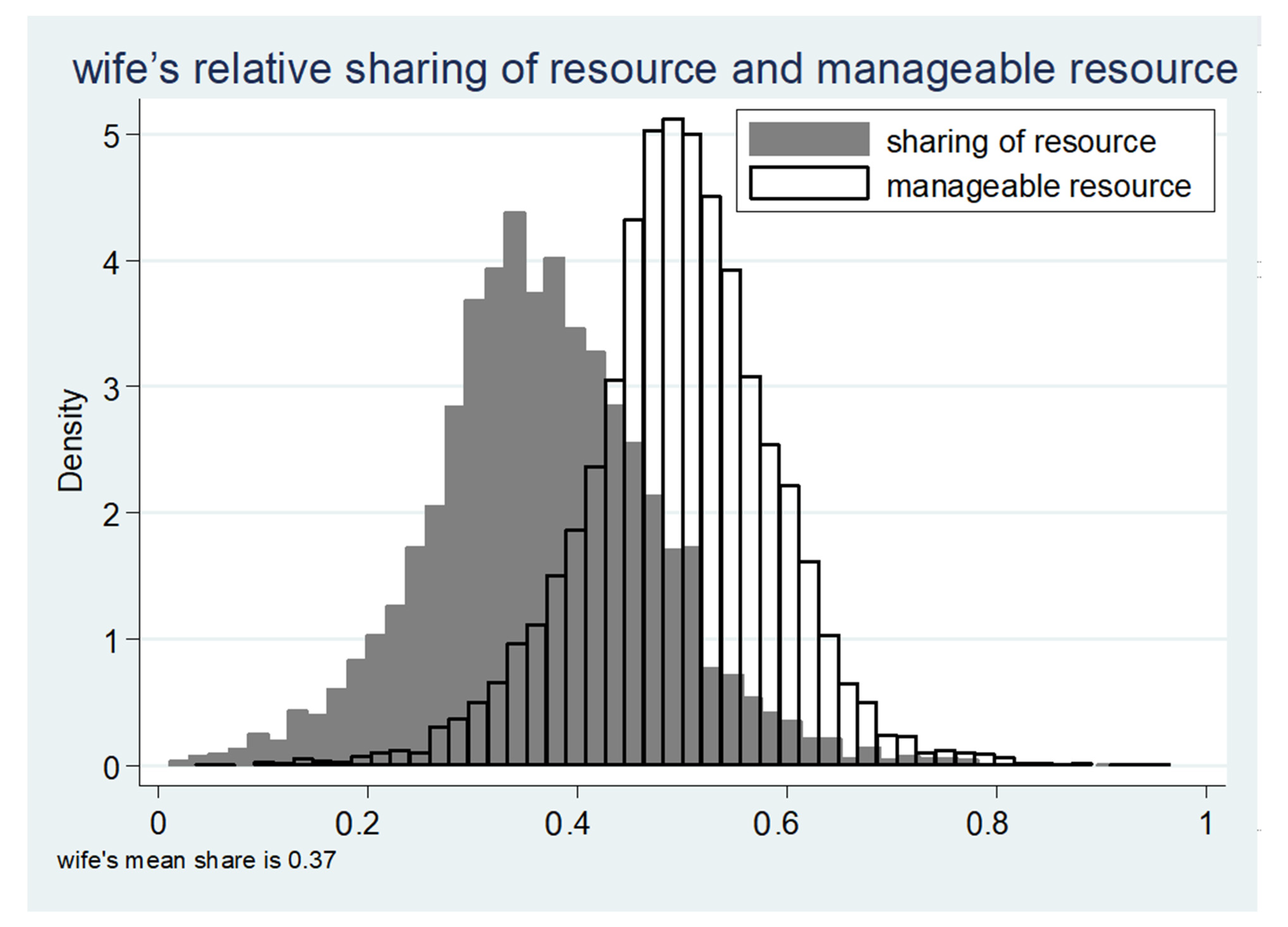
The results of this study are as follows: first, the positive relationship between the wife’s share of intra-household income and her manageable income resources is confirmed. In other words, the more manageable the wife’s income, the more she can determine how to spend these income resources. However, it is notable that although the wife’s manageable full income is almost 50% of the total household’s full income, it does not indicate that the income can be expended by the wife freely based on her preference. To the best of our knowledge, this is the first result to uncover the relationship between manageable income and bargaining power within the family.

Second, based on the estimation results, the wife, on average, shares 37% of the intra-household income resources earned by the couple, while the husband shares 63%. This result indicates that the wife’s relative bargaining power (proxy of the sharing of resources) is weaker than her husband’s. The results of these studies are consistent with the individual levels of resource sharing [10] and therefore make poverty observable at the individual level rather than at the household level. Similarly, previous studies [9,11,32] conclude on the intra-household income allocation inequality and recommend reducing the intra-household resource sharing gap in order to decrease the gender wage gap [9]. This study’s results align with these previous studies; overall, if we want to reduce the intra-household resource-sharing gap, decreasing the gender wage gap is a tool.

Using the intra-household income management information, this paper develops a specification to estimate the sharing rule (or relative sharing of resources). A two-step estimation process has been adopted that estimates the wife’s manageable income equation first. The parameters are substituted in the husband’s income manageable income equation to estimate the parameter for calculating the wife’s sharing rule. The wife’s sharing rule is finally obtained by simulation from the income management and estimated parameter. The determinant factors of the sharing rule (a proxy for welfare) are borrowed from Chiappori [8] and they also determine the relative bargaining power. They are the husband’s wage, the wife’s wage, the household non-labor income, the gender ratio, and the divorce ratio. The results indicate the improvement of the intra-household income allocation inequality associated with household involvement in the natural environment sustainability. The wives’ increase in the ratio of their income to the total household’s income improves the household environment conservation activities.

The policy implications based on the results are summarized. The wife’s share of intra-household resources is positively correlated to her manageable income resources. For instance, increasing a wife’s wage increases both her manageable household income resources and her share of these resources. In other words, the more manageable income the wife has, the more she can determine how to spend these income resources. This finding provides a kind of indication, which is the simplified observation of the household member’s shared resources and even the change in the shared resources. However, wives have a weak bargaining power on the income transferred from their husbands; the results suggest that the increase in the income transfer may not be the key solution to solving the intra-household inequality between husbands and wives. Narrowing the gap in terms of hourly wage between husbands and wives is a crucial tool to reduce the intra-household allocation gap.

Moreover, empirical evidence shows the potential bias caused by assuming identity utility functions within the wives’ and husbands’ groups. The wife, on average, shares 37% of the total intra-household full income, which indicates that the wife’s bargaining power (proxy of the sharing of resources) is weaker than her husband’s, as the husbands share 63% of their income. Since we still observed that wives, on average, share fewer resources than their husbands, adopting the collective model proposed by Chiappori [1] is suggested.

The limitations of this study are summarized as follows. This study presents the intra-household income allocation to identify whether there is an inequality in intra-household income. First, there is an assumption of a positive linear correlation between a family member’s observable manageable income resources and his or her shared income resources. The positive linear correlation assumption may not closely capture the true relationship between these two variables. For example, households may choose different types of intra-household management. A husband may choose to transfer all of his disposable income to his wife and receive pocket money from her; another husband may choose to transfer some of his income to his wife and not receive pocket money. These two types may have different correlations between observable manageable income and shared resources. Therefore, we need to consider the heterogeneity problem between the two variables.

Second, only working wives and husbands were selected for this study. At the same time, non-working individuals are excluded since hourly wages cannot be directly calculated from non-working individuals. This may cause a sample selection problem. Therefore, we will need to estimate the hourly wage for non-working individuals using a developed methodology in future work.