Abstract
Given the effort to reduce greenhouse gas (GHG) emissions, understanding the consumption patterns that facilitate and support changes is essential. In this context, household food consumption constitutes a large part of society’s environmental impacts due to the production and solid waste generation stages. Hence, we focus on applying the Life Cycle Assessment to estimate Brasilia’s GHG emissions associated with household food consumption. We have used microdata from the Personal Food Consumption Analysis to address consumption patterns. The life cycle approach relies on the adaptations for Brasilia’s scenario of the inventories available in the databases of Ecoinvent 3.6 Cutoff and Agribalyse 3.0.1. Individuals’ GHG emissions results were classified according to sociodemographic groups and dietary patterns and analyzed through Analysis of Variance (ANOVA). The results indicate that household food consumption contributes 11,062.39 t CO2e daily, averaging 5.05 kg CO2e per capita. Meat consumption accounts for the largest share of emissions (55.27%), followed by beverages (18.78%) and cereals (7.29%). The ANOVA results indicate that individuals living in houses, individuals between 45 and 54 years old, and men have a higher carbon footprint. Therefore, future analyses for potential reduction should incorporate these target groups. Regarding dietary patterns, vegan individuals contribute 3.05 kg CO2e/day, 59.00% fewer emissions than omnivorous people. The no red meat, pescatarian, and vegetarian diets also imply lower food-related GHG emissions.
1. Introduction
Along with the development of major cities, human activities have intensified, leading to a shift in the scale of the environmental impacts ranging from sectors or countries to global proportions. There has been a transformation in consumption habits regarding quantities and types of products. If current trends continue, the planet’s natural resources will be critically endangered, requiring the resources of two planets to meet the demand [1,2].
Among the significant impacts of human activities is the atmospheric emission of greenhouse gases (GHG), which cause the warming of the planet’s surface. The anthropic influence on the climate has been the leading cause of global warming observed since the mid-twentieth century [3]. The GHG emissions associated with urban activities represent between 60% and 80% of combined emissions. In comparison, the habits of 10% of the world’s population that concentrates most income contribute half of the atmospheric carbon emissions [1].
Compared to levels before the Industrial Revolution (between 1850 and 1900), the average global surface temperature in the decade between 2006 and 2015 indicated a growth of 0.87 °C. Anthropogenic global warming corresponds to about 20% of the total increase, rising by 0.2 °C every decade due to past and ongoing emissions [4].
Aiming to limit GHG emissions and, consequently, the increase in the average temperature of the Earth’s surface, the 21st Session of the Conference of the Parties to the United Nations Framework Convention on Climate Change was held. As a result, the Paris Agreement (PA) was signed between the Parties [5]. The PA’s targets is to encourage the international response to climate change, including limiting the rise in global average temperature to 1.5 °C above the pre-industrial level.
The Parties agreed to achieve the global peak of GHG emissions as soon as possible and balance anthropogenic emissions and sinks [5]. In the context of reducing climate change, Brazil has defined its Nationally Determined Contribution through the National Policy on Climate Change [6]. Consequently, the Brazilian government has voluntarily committed to reducing projected GHG emissions by between 36.1% and 38.9% by 2020.
In terms of GHG emissions, the participation of household consumption is undeniable. Residential consumption is estimated to contribute 13% to 35% of total direct emissions associated with country boundaries. If indirect emissions are considered, households can contribute more than 60% of a country’s air pollution [7].
About 75% of per capita GHG emissions in household consumption are associated with food, transportation, or housing. Furthermore, residential consumption in Brazil contributes 2.8 t CO2e/person annually, of which 1.0 t CO2e/person is related to food [8].
Observing food’s life cycle, the production, processing, marketing, consumption, and disposal stages have significant environmental externalities due to energy demand and extraction of natural resources and their associated GHG emissions [9,10]. However, studies analyzing the contribution to carbon emissions by food consumption are still scarce in the literature. Many studies focus on analyzing the GHG intensity of food production processes by the Life Cycle Assessment (LCA) [11] and the related Carbon Footprint (CF) [12,13,14,15]. However, it is not clear which sociodemographic and household characteristics are associated with a higher demand. Amongst those, several research studies have been conducted to assess the impacts of food consumption in European countries [16,17,18,19,20], the United States [21], India [22], China [23], and Canada [24].
In Latin America, the literature has recently focused on studying the carbon impacts of food consumption. For example, a research study evaluated Chile’s carbon footprint and nutritional habits [25]. Another study investigated GHG emissions from the Mexican diet and identified sociodemographic groups with the highest carbon footprints [26]. In Brazil, research has mainly been using the 2008′s Brazilian Household Budget Survey (POF, from the Pesquisa de Orçamentos Familiares, in Portuguese) to estimate food habits and the resulting GHG emissions [27,28,29,30]. However, studies of food GHG emissions considering recent expenditure and consumption data are still scarce in Brazil. In addition, to our knowledge, analysis of dietary patterns is not available in the country.
In this context, considering the importance of the food sector for GHG emissions and aiming to fill the gap in research estimating the impacts of dietary patterns in Brazil, as well as the need for analysis considering recent data, this work consists of an estimation of GHG emissions associated with household food consumption in Brasilia. Specifically, the research objectives are described as follows: (i) to estimate the contribution of household food consumption in Brasilia to the GHG emissions; (ii) to investigate the influence of sociodemographic variables (income, age, gender, household type) in an individual’s food-related GHG emissions; and (iii) to compare GHG emissions from individuals with different dietary patterns (omnivorous, no beef, no pork, no red meat, pescatarian, vegetarian, and vegan).
2. Study Area
Brasilia was founded in 1960 to be the federal capital of Brazil. The city is in Brazil’s Midwest Region, at 15°47′ S and 47°56′ W, and approximately 1000 m above mean sea level. The city area is 5779 km2, divided into 33 Administrative Regions (ARs) officially constituted by the Federal District Government [31].
Brasilia is the fourth most populous city in the country [31]. According to the Brazilian Institute of Geography and Statistics [32], the estimated population of Brasília in 2021 was 3,079,879 inhabitants. The current demographic density is 444.66 people/km2 [31].
Women are the most significant part of Brasilia’s population, accounting for approximately 52% of all income groups. Regarding the distribution of earnings, most of the population (32%) is in the family income range between 2 and 5 minimum wages, followed by the ranges with monthly income greater than 1 and less than 2 minimum wages (20%), between 5 and 10 minimum wages (17.6%), more than 10 to 20 minimum wages (12.5%), up to 1 minimum wage (10.8%), and more than 20 minimum wages (6.9%) [33].
Regarding the accommodation type, Brasília’s population is distributed as follows: 69% in houses and 28.6% in apartments. The other household types account for only 2.4% [33]. According to data from the 2010 Demographic Census [34], the urban population of Brasília is 96.6%, with a total of 2,482,210 inhabitants in urban centers in the reference year.
Under food consumption, 59.4% of people’s total expenditures from Brasilia are related to it [35]. However, this varies across families’ incomes, ranging from 49.1% for high income (more than R$23,850.00) to 75.3% for lower income (between R$1908.00 and R$2862.00).
3. Methods
3.1. Data Collection
Food consumption data were estimated using the Household Budget Survey 2017–2018 (POF, from the Pesquisa de Orçamentos Familiares, in Portuguese) developed by the Brazilian Institute of Geography and Statistics [35].
Microdata were collected from the results of the personal food consumption block in the survey, from which household data of foods expressed in kilograms consumed were extracted. The data collected reflect two non-consecutive days of consumption of the individuals selected for the survey. The microdata reading and subsequent analysis were performed on the software RStudio 3.6.1, while the entries relating to atypical days of consumption were excluded from the data set. Thus, the answers of 843 individuals distributed in 353 households were considered.
Considering the substantial number of food items mentioned by POF respondents in Brasilia (1860 items in total, 681 recorded in the study area), consumption data were compiled in food groups. The list of food items in each group is available in the Supplementary Materials.
We estimated the total household consumption of each food group by the product between personal consumption within the group and the weight corresponding to each household interviewed in the POF, according to Equation (1) below.
where Cx is the total consumption of food group x (t/day) by the population of Brasilia; aij is the consumption of food i by individual j (kg/day); and Pj is the expansion factor (weight) attributed to the household to which individual j belongs.
All data entries referring to water consumption were excluded from the aggregation. This exclusion is justified since food data used in this research were unsegregated in tap and bottled water. In that case, water consumption in Brasilia represents 45.49% of all items listed in the POF. Therefore, if tap water is considered, the beverage group will account for 62% of the total food consumption. In addition, besides the package production being substantial in terms of GHG emissions, drinking water production is a minor emission process (see the Supplementary Materials).
Regarding the socioeconomic data, the microdata of the characteristics of households and residents were used. The information selected to characterize the population was: household status (urban or rural), type of residence (house, apartment, and others), age, gender, household income, and per capita disposable income. Furthermore, the variables of family income and disposable income per capita were unified according to the value in the 2017 minimum wages (MW) in BRL: (i) up to 1, (ii) between 1 and 2, (iii) between 3 and 5, (iv) between 6 and 10, and (v) more than 10. In addition, the age of the respondents was classified into the following ranges: (i) up to 24 years, (ii) 25–34 years, (iii) 35–44 years, (iv) 45–54 years, (v) 55–64 years, and (vi) more than 65 years.
Finally, to compare the effect of different dietary patterns on food-related GHG emissions, POF respondents were classified according to their self-reported food consumption. Seven dietary groups were considered, as described below. Table 1 contains the food items restricted to each diet by food group. The complete list of food items included in each dietary pattern is available in the Supplementary Materials.

Table 1.
Food is restricted for each dietary pattern. If an individual reported consumption of a restricted item for a diet, they could not be classified as having this dietary pattern.
- Omnivorous: individuals who did not indicate restrictions on food consumption.
- No beef: individuals whose only restriction is “I do not eat cattle meat.” Those individuals indicated consuming all other food items except bovine meat.
- No pork: individuals whose only restriction is “I do not eat swine meat.” Those individuals indicated consuming all other food items except swine meat.
- No red meat: individuals whose restriction is “I do not eat red meat.” Those individuals indicated the consumption of all other food items except red meat (e.g., cattle meat, swine meat, lamb meat, amongst others).
- Pescatarian: individuals whose animal protein consumption comes only from fish.
- Vegetarian: people whose dietary pattern includes all plant-based food, eggs, and dairy products.
- Vegan: people whose eating pattern is composed only of plant-based items.
3.2. Estimation of GHG Intensity
An application of the Life Cycle Assessment (LCA) was carried out according to ISO 14040 [36] and ISO 14044 [37] to estimate the GHG emissions related to each food item.
3.2.1. Scope Definition
The functional unit adopted for the LCA application in this paper was “kg of food consumed” [kg−1]. For the system boundaries, activities from pre-planting ingredients, including fertilizer and pesticide production, were considered. In addition, farm operation, transport to processing centers, processing itself (where applicable), and transportation to retail centers were included (see Figure 1). On the other hand, the products’ storage and household food preparation were not considered. Moreover, household solid waste management was not included since the solid waste generation rate resulting from food preparation and food waste remains unknown.
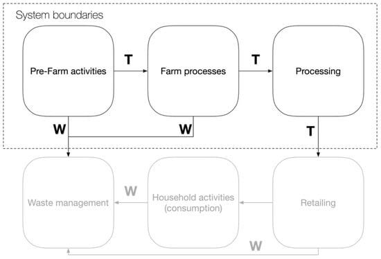
Figure 1.
LCA system boundaries. Stages in black are included in the analysis; stages in gray are excluded. T = transport between stages of the life cycle. W = waste generated in the life-cycle stage. Note: Waste management from pre-farm and farm activities was included in the analysis.
3.2.2. Life-Cycle Inventory
This study’s life cycle inventories (LCIs) analyzed the input and output flow of materials and energy at each stage covered by the system boundaries. In addition, Global (GLO), Brazilian (BR), and “rest of the world” (RoW) inventories available in the Ecoinvent 3.6 Educational Version for non-OECD countries [38] and the Agribalyse 3.0.1 [39] databases were used in this study. To this end, the Ecoinvent Cut-off model was adopted in this work, considering that the waste generated in production processes is treated, and that the treatment burden is fully assigned to the production activity.
The compilation of the data and the construction of the LCI for each food were performed in OpenLCA 1.10® software.
The average transport distances between the producing municipality and the Supply Centers (CEASA) were calculated according to data from the Agricultural Information Portal of the National Supply Company (CONAB, from Companhia Nacional de Abastecimento, in Portuguese) [40]. The average distance was calculated by weighting the distance between the farm’s location and the distribution center in Brasilia by the amount of food, according to Equation (2). The distance estimates for each item are available in the Supplementary Materials.
where Dmed is the average distance between the farm and the distribution center (km); di is the distance between the i-th producing municipality and the distribution center in Brasilia (km); and Qi is the amount of food originating from the i-th city (kg).
When applicable, differences between the farm (or processing site) and the distribution centers for food items not included by CONAB [40] were obtained through the inventories available in the Ecoinvent 3.6 and Agribalyse 3.0.1 databases.
An adjustment of the energy matrix on the processes associated with the product life cycle was made to adapt Ecoinvent 3.6 inventories to the Brazilian scenario. Since most of the food production processes available in the database referred to the European Union, and considering the differences between the European and Brazilian energy matrices, it was necessary to perform such an adaptation. The details of all the adaptations made are available in the Supplementary Materials.
3.2.3. Life-Cycle Impact Assessment
The Life-cycle Impact Assessment (LCA) was carried out according to the CML-IA 2001 baseline methodology [41] for the impact category of global climate change. The result of GHG emissions was expressed in kilograms of carbon dioxide equivalent (kg CO2e). In a given time horizon, the conversion factors of other gases, such as methane and nitrous oxide, are defined by the Global Warming Potential (GWP). In this work, GWP100 was used, referring to the global warming potential over a time horizon of 100 years (GWP100a). In this case, OpenLCA 1.10® software was used to perform the LCIA.
The resulting GHG emissions were aggregated into the food groups according to the classification available in the Supplementary Materials. For each individual, GHG emissions by food group and total emissions were aggregated through Equations (3) and (4), respectively.
where GHGk is the GHG emissions by the k-th food group (kg CO2e.day−1); ai is the consumption of the i-th food item (kg food.day−1); Ii is the intensity (kg CO2e kgfood−1); and GHGj is the total emissions by the j-th individual.
3.2.4. Statistical Analysis
The statistical analysis of the data set was performed on the RStudio 3.6.1 software. Descriptive statistics were used to characterize the sample’s sociodemographic data, including household status, type of residence, age, gender, household income, and per capita disposable income. In the second stage, the Analysis of Variance (ANOVA) was used to compare the differences between GHG emissions and food consumption for the sociodemographic groups. Furthermore, the GHG emissions from different dietary patterns were also compared through ANOVA.
4. Results and Discussion
4.1. Sample Characteristics
As described in Section 3.1, after removing the responses referring to atypical days, the sample used in this work included data from 843 individuals in 353 households. Table 2 contains the main descriptive statistics for the sample used.
Table 2.
Sample descriptive statistics.
It was observed that, regarding age, most respondents are up to 24 years old (220 individuals, 26.10%). Age groups 25–34, 35–44, and 45–45 are similarly distributed, with 138 (16.37%), 148 (17.56%), and 140 (16.61%) individuals each, respectively. The sample included a small fraction of older individuals—105 between 55 and 64 years (12.46%) and 92 over 65 years (10.91%). The mean age of the individuals was 39.35 years, and the median was equal to 39 years.
According to CODEPLAN [33], the distribution of the Brasilia population is 36.00% up to 24 years old, 15.82% between 25 and 34 years old, 16.47% between 35 and 44 years old, 13.48% between 45 and 54 years old, 9.38% between 55 and 64 years old, and 8.86% aged 65 years or older. Thus, the average age is 33, with a median of 34.71.
Although there is a more than 5% difference between the sample and the population of Brasília in the proportion of individuals under 24 years old, the other age groups are similar. Hence, the sample utilized in this study can be considered heterogeneous regarding age.
In terms of gender, individuals’ distribution in the sample (F: 52.57%) is approximate to the proportion of the population of Brasilia (F: 52.20%) [33]. The sample is predominantly urban regarding household status, with 727 individuals (86.24%) residing in 310 (87.82%) urban domiciles. According to the 2010 IBGE Census [34], 96% of the city’s population resides in urban areas.
The distribution of household types also has a group with strong dominance: people living in houses (single-family dwellings). There are 717 individuals (85.05%) residing in houses, with 115 (13.64%) living in apartments and 11 (1.30%) in other types of dwellings (rooming houses and tenements, among others). The distribution of active residences in Brasilia has houses as the predominant group, with 69.0%, followed by apartments, with 28.6% of the population [33]. The other types of domiciles represent 2.4% of the city’s population.
Finally, the distribution of individuals by income was analyzed according to total family and per capita household income. Although most individuals (294 occurrences, 34.88%) are in families with a total income greater than 10 minimum monthly wages, households are more distributed. There are 105 (29.75%) in the highest income bracket, 99 (28.05%) between 3 and 5 minimum wages, and 96 (27.20%) between 6 and 10 minimum wages.
In Brasilia, the average monthly household income tends to be between 2 and 5 minimum wages, with 32.0% of the total [33]. Next, there are the ranges between 1 and 2 salaries (20.0%), more than 10 salaries (19.4%), and up to 1 minimum wage (10.8%). On the other hand, when the variable analyzed becomes the per capita income, most individuals are in the 1 to 2 income brackets (269 individuals, 31.91%) and the 3 to 5 minimum wages bracket (252, 29.89%). Regarding households, the two ranges are still predominant but in reverse order. There are 105 homes (29.75%) with an average per capita income between 3 and 5 minimum wages and 101 homes (28.61%) with an income between 1 and 2 minimum wages.
4.2. Food Consumption
The weighted total daily food consumption in Brasilia and the average household consumption per capita are in Table 3.
Table 3.
Household food consumption in Brasília.
The results showed that the total food consumed in Brasilia’s households on typical days was 4342.483 t daily. The leading group is beverages, representing more than 30% consumed (kg). However, it should be noted that, even without including water consumption in this group, it still constitutes the most considerable fraction of food consumption in Brasilia.
Within the beverage food group, the subgroup most consumed is coffee, with 495.54 t (37.59% of the group, 11.41% of the total), followed by juices, with 373.32 t (28.32% of the group, 8.60% of the total) and soft drinks, with 194.98 t (14.79% of the group, 4.49% of the total).
The consumption of cereals, meat, and legumes also stands out, with 11.444%, 11.324%, and 10.389%, respectively, of the total food indicated in the POF. Regarding cereals, the most substantial contribution comes from the rice subgroup, with 417.97 t (84.10% of the category). Next comes the corn and corn-based preparations subgroup, with 43.27 t (8.70% of the category). Regarding meat, 36.24% of the total group corresponds to beef, with 178.21 t consumed. Poultry and pork also contribute significantly, with 152.72 t (31.06% of the group) and 51.74 t (10.52% of the group), respectively. Finally, regarding legumes, beans and bean-based preparations represent almost the entire group, with 399.64 t (88.58%) and 38.391 t (8.51%), respectively. The complete list of the fraction corresponding to each subgroup in the total food consumed is available in the Supplementary Materials.
4.3. GHG Emissions
The total GHG emissions of the food groups and the per capita emissions of the population of Brasilia are available in Table 4.
Table 4.
GHG emissions related to food consumption in Brasília.
On a typical consumption day, it was estimated that the GHG emissions associated with food consumption in Brasilia’s households are 11,062.39 t CO2e. Furthermore, the results indicated an average per capita emission of 5.05 kg of CO2e/day. This portion of the emissions was more significant than the fraction related to mobility in the city which, in 2016, corresponded to 3.63 kg of CO2e/person/day [42].
Compared to similar studies, the results obtained in this research evidence that individuals in Brasilia contribute significantly to GHG emissions. For instance, GHG emissions due to food consumption in Japan have been estimated at 3.84 kg CO2e/person/day [43] while, in Finland, estimates range between 3.84 kg CO2e/person/day [44] and 4.79 kg CO2e/person/day [43]. Brasilia’s food-related GHG emissions were also more significant than other countries in Latin America. In Chile, daily emissions ranged from 2.42 to 4.74 kg of CO2e/person/day [25] whereas, in Mexico, the food carbon footprint implies 3.9 kg of CO2e/person/day [26]. However, some places still show higher GHG emissions per capita than Brasilia. For example, while in Argentina the diets averaged 5.48 kg CO2e/person/day [45] of GHG emissions, Toronto contributes 6.03 kg of CO2e/person/day [24]. In the United States, individuals with a standard diet could release 8.14 kilograms of CO2e daily [46]. Previous research also indicates that average daily GHG emissions from food consumption in Brazil range from 4.49 [30] to 6.67 [28] kilograms of CO2e per person.
It is observed that the beverages food group accounts for 30.35% of the total food consumed in Brasilia (Table 2). This fraction corresponds to 18.78% of the total GHG emissions, with an average intensity of emissions of 1.576 kg CO2e/kg of food. In this scenario, the medium-high intensity of beverages can be explained by the inclusion of glass, plastic, and metal packaging impacts in the processing stage of the life cycle (see the system boundaries in Figure 1).
On the other hand, meat represents 11.32% of the total food consumed and contributes to 6,114.61 t of CO2e. This amount results in 55.27% of GHG emissions from household food consumption in the region. These results are aligned with previous research [27] that indicated meat consumption as the leading cause of food-related GHG emissions.
The high intensity of GHG emissions related to meat consumption is due to beef, whose production involves 24.47 kg CO2e/kg. Furthermore, pork contributes 6.9 kg CO2e/kg, and poultry with 2.10 kg CO2e/kg—combined with beef and other items within the group—results in an average intensity of emissions of 12.43 kg CO2e/kg of meat.
Fish have low GHG emissions within the animal proteins (meat). The consumption of fresh, canned, and salted fish results in 76.22 t CO2e (0.69%), 7.42 t CO2e (0.07%), and 9.232 t CO2e (0.08%), respectively, with intensities of 2.793 kg CO2e/kg, 4.892 kg CO2e/kg, and 2.472 kg CO2e/kg, respectively.
Subsequently, when it comes to reducing the impact of food consumption on climate change, replacing beef with low-carbon proteins can be an option. Just for comparison purposes, if beef (178.21 t) was replaced by 50% of poultry (GHG emissions intensity 2.01 kg CO2e/kg) and 50% of fresh fish (2.79 kg CO2e/kg), the total GHG emissions of household food consumption in Brasilia would be reduced from 11,062.39 t CO2e to 7138.45 t CO2e, a 35.47% reduction.
While the contribution of food consumption patterns to GHG emission is a critical analysis element, understanding the carbon intensity estimations based on the Life Cycle Assessment framework is necessary. Brasilia’s urban and rural planning does not consider the inclusion of industries, relying extensively on goods and services provided by several locations across the country. This scenario has implications for the system boundaries assessed in this study in terms of territorial extent on the intensity values, which fully incorporates the contribution of transporting goods by road across several locations in the country. Therefore, the increase in the carbon intensity of food is noticeable with meat from the state of Minas Gerais. Vegetables such as potatoes are mainly produced in the states of Minas Gerais and Goiás, located at an average distance of 509 km. Apples are shipped from Santa Catarina and the Rio Grande do Sul states at 1.611 km. Carbon intensity modeling incorporates the question of how to relate the contribution of post-consumption of food to waste disposal, representing around 60% of the municipal solid waste composition. As modeled in previous studies, Brasilia’s municipal solid waste management system shifted from using open dumps to landfilling without biogas recovery, thereby extensively contributing to methane emissions [47].
Recognizing the significance of shifting food consumption towards low-carbon alternatives will improve the overall footprint. For example, choosing a different source of proteins, or eating fewer insensitive meat alternatives, such as pork and poultry, will help reduce the contribution to GHG emissions. According to our LCA analysis, red meat (beef) has an intensity of 24.47 kg CO2e per kg compared to poultry with 2.10 kg CO2e per kg, similar to previous research [48]. However, in some cases, such as meat production, it is necessary to analyze the policy implications of such changes extensively since several regions in the country rely on this industry.
The effect of reducing consumption is uncertain; while this might lead to savings, it will also have a rebound effect since it might lead consumers to spend on other goods with a higher footprint. Although these outcomes are possible, as discussed above [49], the secondary effects of the rebound effect are less defined since they incorporate a series of effects ranging from behavioral to technological spillover.
4.3.1. GHG Emissions by Sociodemographic Groups
Exploratory statistical analyses were performed on the results of GHG emissions. These results were compared regarding family income, per capita income, household situation, type of household, age group, and gender of the respondents. The average emissions by group are presented in Table 5.
Table 5.
Average GHG emissions for each sociodemographic subgroup of Brasilia’s population.
Our findings identified key groups for future climate change mitigation actions by focusing on multiple comparisons between clusters of individuals with similar socioeconomic variables and food consumption patterns.
First, there were significant differences in GHG emissions between individuals according to age and gender variables. Regarding age, the most meaningful average emissions were found in individuals between 45 and 54 years old, followed by those between 35 and 44. The lowest mean emission was registered for individuals older than 65. However, despite the differences in the means between the age groups up to 24 years, 25–34 years, 35–44 years, and 45–54 years, an application of Tukey’s test with a 95% confidence interval did not show differences between these groups. Only the age groups between 45–54 years and ≥65 years and between 55–64 years and ≥65 years showed sufficient statistical differences. Hence, it can be inferred that GHG emissions associated with food consumption in Brasilia decrease as individuals advance beyond 65. Furthermore, the highest level of food emissions occurs in individuals between 45 and 54 years.
As for gender, the average for respondents identified as “male” (7.06 kg CO2e/individual) was about 27% higher than that of individuals identified as “female” (5.15 kg CO2e/individual). This difference can be explained by the higher consumption of food by men, especially of meat (0.30 kg/person by men, 0.22 kg/person by women), cereals (0.30 kg/person by men, 0.21 kg/person by women), and legumes (0.30 kg/person by men, 0.19 kg/person by women).
Regarding income, no sufficient evidence was found to reject the hypothesis of equality between total GHG emissions for family income and per capita income variables. This result probably occurred because the range of GHG emissions is comprehensive for all income groups.
We subsequently analyzed the average individual GHG emissions by food group according to previously used sociodemographic variables. Table 6 contains the key results of the Two-Way Analysis of Variance (ANOVA) between the groups formed according to household income, per capita income, household status, type of residence, age, and gender for each food category.
Table 6.
ANOVA results for the comparison of GHG emissions.
For household and per capita income, the cereal and legume groups have higher emissions for the lowest income bracket (up to one minimum wage). This outcome is due to the diet of individuals with lower family income, primarily made up of staple foods such as rice and beans.
On the other hand, dairy-related emissions are lower for this group of individuals (income < 1 MW), and the median increases as family income increases, indicating increased consumption of these items. Dairy products contribute, on average, 2.21 kg CO2e/kg of food (Table 3). However, while milk has an average intensity of GHG emissions of 1.41 kg CO2e/kg, items such as cheese are more impactful, with 10.74 kg CO2e/kg. Consequently, dairy-related emissions might be even more considerable in higher-income groups due to differences in the quantities and items consumed.
Observing the results of GHG emissions by food group according to household status, five of them showed statistically different averages between rural and urban areas: dairy products, vegetables, eggs, beverages, and pulses.
Among the food categories mentioned above, the average GHG emissions were higher for people domiciled in urban areas, but only for dairy products and eggs. For the others, the contribution of rural households to climate change was more notable.
Considering the average food consumption data by food category (Table 2), the categories beverages, vegetables, and legumes were consumed more by individuals living in rural areas, which explains the higher emissions of those for these categories. Similarly, dairy products and egg consumption are more significant in urban areas, generating higher emissions for this type of household.
Regarding the household type, individuals grouped into houses, apartments, and other types showed different averages for meat, cereals, dairy products, and snacks. For meat, although the median emissions are higher for households classified as other, the average consumption for the houses is higher (Table 4). Therefore, the emissions values related to meat consumption are more distributed to single-family dwellings. The differences in GHG emissions related to meat consumption between individuals living in houses and apartments can be explained by the higher meat consumption by individuals residing in houses, as shown in Table 2 and Table 3. For cereals, as for meats, the median GHG emissions are higher for houses, although the median is higher for the “other” group. In parallel, consumption in this category is higher for households, and the pairwise comparison did not allow a comparison of houses and apartments with other types of households. On the other hand, for dairy products and snacks, the average GHG emissions are higher for individuals living in apartments due to the higher consumption of items in this category.
As for the age group of the POF respondents, the GHG emissions showed differences between the averages of the food groups for two of the most impacting categories: meat and beverages. For beverages, age group pairs ≤ 24 and 45–54 (p-value < 0.00001) and <24 and 55–64 (p-value < 0.00001) showed statistically different GHG emissions averages from each other. Of these, the 45–54-year-old group had the highest mean, with 1.32 kg CO2e/person, followed by 55–64-year-old individuals, with 1.25 kg CO2e/person. The lowest GHG emissions are associated with the lowest age group (up to 24 years), accounting for 0.68 CO2e/individual. Variations in consumption can explain the differences between these groups. Therefore, the groups that produce fewer emissions consume less, and vice versa (see Table 2 and Table 3), although some variations in beverage consumption were not reflected in GHG emissions.
For example, individuals between the ages of 35 and 44 are responsible for the highest beverage consumption. However, the group with the highest GHG emissions is between 45 and 54 years old. Therefore, these divergent fluctuations might be explained by differences in consumption patterns between these age groups. The groups with higher total category consumption and lower emissions consume, on average, foods with less intense climate change impacts. The same analysis can be employed for meat, where statistical evidence of differences between averages was found exclusively for groups over 65 and between 45 and 54 years old. Although, in absolute terms, the group with the highest consumption (45–54 years old) showed higher average emissions, the difference between the average consumed between the two groups was 24.17% (compared to the group between 45 and 54 years old), the difference between the average emissions was 49.03%. Therefore, it can be concluded that there was a variation in the total consumed between the age groups. On the other hand, there was a change in the foods consumed so that the 45–54 age group chose items with a higher pollution intensity, such as beef.
In conclusion, considering the gender of the respondents, men and women had different average GHG emissions in the beverages, meat, cereals, sweets, fruits, legumes, and eggs groups, all due to the proportional increase in consumption in the respective categories compared to females.
4.3.2. The Effect of Dietary Patterns on GHG Emissions
The purpose of this research is to characterize the effect of different dietary patterns (omnivorous, no beef, no pork, no red meat, pescatarian, vegetarian, and vegan) on the contribution to GHG emissions. The results of this analysis can be observed in Figure 2. Individuals with a self-reported vegan diet are responsible for the lowest average GHG emissions (3.05 kg CO2e/day), followed by no red meat (3.07 kg CO2e/day), pescatarian (4.48 kg CO2e/day), and vegetarian diets (4.57 kg CO2e/day). On the other hand, people with omnivorous (7.44 kg CO2e/day), no pork (7.01 kg CO2e/day), and no beef (4.61 kg CO2e/day) diets have the higher food-related contribution to climate change. The ANOVA results confirmed significant differences between the dietary groups (p-value < 0.0001). An application of Tukey’s test with a 95% confidence interval showed statistical evidence that the average emissions of omnivorous and no pork diets are higher than vegan, vegetarian, no beef, and no pork diets (p-value < 0.05).
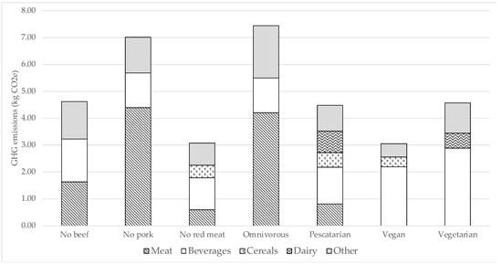
Figure 2.
Average food-related GHG emissions for seven dietary patterns of Brasilia’s population. Meat, beverages, cereals, and dairy are the main food groups contributing to GHG emissions. All other food groups with <10% of the group emissions are represented as “Other”.
When analyzing the results associated with the dietary pattern, meat, and dairy consumption play a significant role in carbon footprint. Vegan and no red meat diets have a lower average emission once there is no consumption of carbon-intense food, i.e., animal-based or red meat. Surprisingly, a vegetarian diet without meat averaged higher GHG emissions than no red meat and pescatarian diets in Brasília. In this case, consuming carbon-intense dairy products such as milk and cheese is responsible for increasing the vegetarian carbon footprint. While a pescatarian diet promotes a transition towards sustainable food habits, this diet does not consider meat consumption different from fish and sea products. Therefore, its GHG emissions are higher than the no red meat diet. The results can be explained by substituting red and poultry meat for fish and, primarily, by dairy products, implying a higher carbon intensity. Therefore, due to consumer choices in Brasília, an effective policy aiming to reduce food contribution to climate change should focus on a transition to the reduction of red meat through promoting the shift to the no red meat diet, a transition which could be less impactful for consumers.
4.4. Limitations
It should be noted that, in this study, the application of the methods included data limitations. First, the analyses included in this research were conducted with secondary data. In this context, some food items could not be assessed since their inventories were unavailable in the databases. In this way, 183 items of food listed in the POF were not considered. Among these items, most correspond to the groups of sweets (64 items), snack foods (47 items), and baked goods (45 items). These groups constitute 0.625%, 1.414%, and 1.032%, respectively, of the food that the residents consume in the sample area. Therefore, the sum of all items not included in the GHG estimates equals 137.93 kg, equivalent to 3.601% of the mass of food consumed. The list of items excluded from the analysis and their respective consumption amounts is available in Supplementary Materials.
Notably, most items not being considered reflect the lack of information about the ingredients used in their preparation or the case of ultra-processed foods, such as cakes, cookies, bread, and sandwiches. On the other hand, some items were included in the analysis using estimates of similar production processes, such as the case of potatoes and cassava. In this case, we suggest further research to reduce the uncertainties, including an extensive collection of primary consumption data.
For the application of the LCA, the definition of system boundaries includes its limitations, given the diversity and complexity of the food production processes included in the analysis. Nevertheless, the system’s boundaries consider a general scope ranging from pre-farm procedures (such as the production of inputs, fertilizers, and soil preparation) to transportation for distribution. To this end, GHG emissions from the distribution stages, consumption (household activities), and waste management generated in consumption were omitted. In this context, the impact of climate change on food consumption in Brasilia presented in this paper is underestimated.
Regarding dietary patterns, as the POF contains data from two consumption days, the classification of people’s diets considers only a short period. Therefore, if an individual reported the consumption of only plant-based food on the POF, but, on most regular days, they eat meat, in this research, they were considered a vegan.
5. Conclusions
In this study, we estimated the GHG emissions resulting from household food consumption in Brasilia, considering the top-down approach by the Life Cycle Assessment methodology. The analysis of the consumption patterns across sociodemographic variables calls attention to the influence of age, sex, and residence type on the overall Carbon Footprint. The results confirmed meat as the food group with a major GHG intensity contribution, as previous studies about food consumption had highlighted over the years. Furthermore, the inventory values show the relevance of direct and indirect emissions analysis and the implications concerning energy requirements based on Brazil’s electricity matrix for 2020, composed of 84.8% renewables [50]. A transversal assessment of fuel consumption across the food category groups plays a key role in understanding the aggregated outcome when considering the country’s continental dimension by the food transportation to the capital. These findings imply that mitigation actions regarding food production should lean toward increasing awareness of sustainable consumption.
Second, the research results identified the sources of variations in GHG emissions associated with food consumption in some groups of individuals. Within households, this contribution is twofold, with men representing the group with the highest average emissions due to food consumption, with about 27% more in the daily contribution to GHG emissions when compared to women. In comparison, it was observed that the group with the most significant emissions coincided with the group with the highest consumption: individuals between 45 and 54 years old when considering meat consumption by age. The analysis of beverage-related emissions by age shows that an increase in consumption was not reflected in the overall emissions. Individuals between 35 and 44 years old were responsible for the highest consumption of beverages; however, the group between 45 and 54 years old had the most significant contribution. Thus, individuals with higher total category consumption and fewer emissions consume foods with lower climate change impacts. Such differences are reflected in the dietary patterns, as vegan and no red meat diets contribute to lower GHG emissions compared to the usual omnivorous and other diets based on meat consumption. While avoiding meat consumption—specifically bovine meat—could reduce GHG emissions, the increase of dairy products on individuals’ food habits has an undesirable effect on the contribution of diets to climate change.
We recommend that further efforts explore the relationship between the intensity of emissions, consumption, and total GHG emissions by category. Comparative studies are also needed to evaluate (i) the difference across dietary patterns of population groups according to age, income, education, and other sociodemographic variables; and (ii) the correlation between consumption and intensity of emissions for each food category.
Supplementary Materials
The following supporting information can be downloaded at: https://www.mdpi.com/article/10.3390/su15076174/s1.
Author Contributions
Conceptualization, V.S.; Methodology, V.S. and F.C.; Validation, R.K.; Formal analysis, V.S.; Writing—original draft, V.S.; Writing—review & editing, F.C., R.K. and C.L.; Supervision, F.C.; Project administration, C.L.; Funding acquisition, C.L. All authors have read and agreed to the published version of the manuscript.
Funding
This research was supported by the Brazilian Coordination for the Improvement of Higher Education Personnel (CAPES, in Portuguese) M.S. scholarship, grant number 88882.383329/2019-01. The APC was funded by Institute for Global Environmental Strategies (IGES) SRF fund 2022.
Institutional Review Board Statement
Not applicable.
Informed Consent Statement
Not applicable.
Data Availability Statement
Publicly available datasets were analyzed in this study. This data can be found here: https://www.ibge.gov.br/estatisticas/sociais/saude/24786-pesquisa-de-orcamentos-familiares-2.html?edicao=28523 (accessed on 2 January 2023). The LCA data presented in this study are available in Supplementary Materials.
Conflicts of Interest
The authors declare no conflict of interest.
References
- Akenji, L.; Chen, H. A Framework for Shaping Sustainable Lifestyles; United Nations Environment Programme: Nairobi, Kenya, 2016. [Google Scholar]
- Brundtland, G.H. Our Common Future. Oxford Pap. Geogr. J. 1988, 154, 116. [Google Scholar] [CrossRef]
- Allen, M.R.; Dube, O.P.; Solecki, W.; Aragón-Durand, F.; Cramer, W.; Humphreys, S.; Kainuma, M.; Kala, J.; Mahowald, N.; Mulugetta, Y.; et al. Global Warming of 1.5 °C an IPCC Special Report on the Impacts of Global Warming of 1.5 °C above Pre-Industrial Levels and Related Global Greenhouse Gas Emission Pathways, in the Context of Strengthening the Global Response to the Threat of Climate Change, Sustainable Development, and Efforts to Eradicate Poverty; IPCC: Geneva, Switzerland, 2018. [Google Scholar]
- IPCC. Working Group III Contribution to the Fifth Assessment Report of the Intergovernmental Panel on Climate Change, Climate Change 2014 Mitigation of Climate Change; IPCC: Geneva, Switzerland, 2014. [Google Scholar]
- United Nations. Paris Agreement. In Proceedings of the 21st Conference of Parties, Paris, France, 30 November–11 December 2015; Available online: https://digitallibrary.un.org/record/831039 (accessed on 19 January 2023).
- Lei n. 12.187, de 29 de Dezembro de 2009. In Institui a Política Nacional sobre Mudança do Clima—PNMC e dá Outras Providências; Diário Oficial da União: Brasília, Brasil, 2009. Available online: https://www.planalto.gov.br/ccivil_03/_ato2007-2010/2009/lei/l12187.htm (accessed on 2 January 2023).
- Wilson, J.; Tyedmers, P.; Spinney, J.E.L. An exploration of the relationship between socioeconomic and well-being variables and household greenhouse gas emissions. J. Ind. Ecol. 2013, 17, 880–891. [Google Scholar] [CrossRef]
- IGES; Aalto University; D-mat Ltd. 1.5-Degree Lifestyles: Targets and Options for Reducing Lifestyle Carbon Footprints; Technical Report; Hayama: Osaka, Japan, 2019. [Google Scholar]
- De Boer, I.J.M.; Cederberg, C.; Eady, S.; Gollnow, S.; Kristensen, T.; Macleod, M.; Meul, M.; Nemecek, T.; Phong, L.T.; Thoma, G.; et al. Greenhouse gas mitigation in animal production: Towards an integrated life cycle sustainability assessment. Curr. Opin. Environ. Sustain. 2011, 3, 423–431. [Google Scholar] [CrossRef]
- FAO. FAO Statistical Yearbook 2020—World Food and Agriculture, Food and Agriculture Organization of the United Nations, World Food and Agriculture—Statistical Yearbook 2020; FAO: Rome, Italy, 2020. [Google Scholar]
- Skunca, D.; Tomasevic, I.; Nastasijevic, I.; Tomovic, V.; Djekic, I. Life Cycle Assessment of the Chicken Meat Chain. J. Clean. Prod. 2018, 184, 440–450. [Google Scholar] [CrossRef]
- Feng, W.; Cai, B.; Zhang, B. A Bite of China: Food Consumption and Carbon Emission from 1992 to 2007. China Econ. Rev. 2020, 59, 100949. [Google Scholar] [CrossRef]
- Kanemoto, K.; Moran, D.; Shigetomi, Y.; Reynolds, C.; Kondo, Y. Meat Consumption Does Not Explain Differences in Household Food Carbon Footprints in Japan. One Earth 2019, 1, 464–471. [Google Scholar] [CrossRef]
- Vita, G.; Lundström, J.R.; Hertwich, E.G.; Quist, J.; Ivanova, D.; Stadler, K.; Wood, R. The Environmental Impact of Green Consumption and Sufficiency Lifestyles Scenarios in Europe: Connecting Local Sustainability Visions to Global Consequences. Ecol. Econ. 2019, 164, 106322. [Google Scholar] [CrossRef]
- Thomas, C.; Maître, I.; Symoneaux, R. Consumer-Led Eco-Development of Food Products: A Case Study to Propose a Framework. Br. Food J. 2021, 123, 2430–2448. [Google Scholar] [CrossRef]
- MacDiarmid, J.I. Is a healthy diet an environmentally sustainable diet? Proc. Nutr. Soc. 2013, 72, 13–20. [Google Scholar] [CrossRef]
- Saxe, H.; Larsen, T.M.; Mogensen, L. The global warming potential of two healthy Nordic diets compared with the average Danish diet. Clim. Chang. 2013, 116, 249–262. [Google Scholar] [CrossRef]
- Sonesson, U.; Mattsson, B.; Nybrant, T.; Ohlsson, T. Industrial processing versus home cooking: An environmental comparison between three ways to prepare a meal. Ambio 2005, 34, 414–421. [Google Scholar] [CrossRef]
- Tukker, A.; Goldbohm, R.A.; De Koning, A.; Verheijden, M.; Kleijn, R.; Wolf, O.; Pérez-Domínguez, I.; Rueda-Cantuche, J.M. Environmental impacts of changes to healthier diets in Europe. Ecol. Econ. 2011, 70, 1776–1788. [Google Scholar] [CrossRef]
- Vieux, F.; Darmon, N.; Touazi, D.; Soler, L.G. Greenhouse gas emissions of self-selected individual diets in France: Changing the diet structure or consuming less? Ecol. Econ. 2012, 75, 91–101. [Google Scholar] [CrossRef]
- Weber, C.L.; Matthews, H.S. Food-miles and the relative climate impacts of food choices in the United States. Environ. Sci. Technol. 2008, 42, 10. [Google Scholar] [CrossRef]
- Pathak, H.; Jain, N.; Bhatia, A.; Patel, J.; Aggarwal, P.K. Carbon footprints of Indian food items. Agric. Ecosyst. Environ. 2010, 139, 66–73. [Google Scholar] [CrossRef]
- Chen, D.D.; Gao, W.S.; Chen, Y.Q.; Zhang, Q. Ecological footprint analysis of food consumption of rural residents in China in the latest 30 years. Agric. Agric. Sci. Procedia 2010, 1, 106–115. [Google Scholar] [CrossRef]
- Veeramani, A.; Dias, G.M.; Kirkpatrick, S.I. Carbon footprint of dietary patterns in Ontario, Canada: A case study based on actual food consumption. J. Clean. Prod. 2017, 162, 1398–1406. [Google Scholar] [CrossRef]
- Franco, C.C.; Rebolledo-Leiva, R.; González-García, S.; Feijoo, G.; Moreira, M.T. Addressing the food, nutrition and environmental nexus: The role of socioeconomic status in the nutritional and environmental sustainability dimensions of dietary patterns in Chile. J. Clean. Prod. 2022, 379, 134723. [Google Scholar] [CrossRef]
- López-Olmedo, N.; Stern, D.; Bakhtsiyarava, M.; Pérez-Ferrer, C.; Langellier, B. Greenhouse Gas Emissions Associated with the Mexican Diet: Identifying Social Groups With the Largest Carbon Footprint. Front. Nutr. 2022, 9, 791767. [Google Scholar] [CrossRef]
- Aguiar, R.D.; Costa, G.N.; Simões, G.T.C.; Figueiredo, A.M. Diet-Related Greenhouse Gas Emissions in Brazilian State Capital Cities. Environ. Sci. Policy 2021, 124, 542–552. [Google Scholar] [CrossRef]
- Travassos, G.F.; Cunha, D.A.; Coelho, A.B. The environmental impact of Brazilian adults’ diet. J. Clean. Prod. 2020, 272, 1226222. [Google Scholar] [CrossRef]
- Garzillo, J.M.F.; Poli, V.F.S.; Leite, F.H.M.; Steele, E.M.; Machado, P.P.; Louzada, M.L.d.C.; Levy, R.B.; Monteiro, C.A. Ultra-processed food intake and diet carbon and water footprints: A national study in Brazil. Rev. De Saúde Pública 2022, 56, 6. [Google Scholar] [CrossRef] [PubMed]
- Garzillo, J.M.F.; Machado, P.P.; Leite, F.H.M.; Steele, E.M.; Poli, V.F.S.; Louzada, M.L.d.C.; Levy, R.B.; Monteiro, C.A. Carbon Footprint of the Brazilian Diet. Rev. De Saúde Pública 2021, 55, 90. [Google Scholar]
- GDF. 2021; About Brasilia [WWW Document]. Available online: http://www.df.gov.br/333/ (accessed on 16 March 2021).
- IBGE. 2021; IBGE|Projeção da População. Instituto Brasileiro de Geografia e Estatística. Available online: https://www.ibge.gov.br/apps/populacao/projecao/index.html?utm_source=portal&utm_medium=popclock&utm_campaign=novo_popclock (accessed on 16 March 2021).
- CODEPLAN. PDAD—Pesquisa Distrital por Amostra de Domicílios 2018, in: Relatório Codeplan. Secretaria de Fazenda, Planejamento, Orçamento e Gestão; Governo Do Distrito Federal: Brasília, Brazil, 2019.
- IBGE. IBGE Censo 2010; IBGE: Rio de Janeiro, Brazil, 2010. [Google Scholar]
- IBGE. POF: 2017–2018: Análise do Consumo Alimentar Pessoal No Brasil; Instituto Brasileiro de Geografia e Estatística: Rio de Janeiro, Brazil, 2020.
- ISO 14040:2006; Environmental Management. Life Cycle Assessment. Principles and Framework. International Organization for Standardization: London, UK, 2006.
- ISO 14044:2006; Environmental Management—Life Cycle Assessment—Requirements and Guidelines—Amendment 1. International Organization for Standardization: London, UK, 2006.
- Wernet, G.; Bauer, C.; Steubing, B.; Reinhard, J.; Moreno-Ruiz, E.; Weidema, B. The ecoinvent database version 3 (part I): Overview and methodology. Int. J. Life Cycle Assess. 2016, 21, 1218–1230. [Google Scholar] [CrossRef]
- Asselin-Balençon, A.; Broekema, R.; Teulon, H.; Gastaldi, G.; Houssier, J.; Moutia, A.; Rousseau, V.; Wermeille, A.; Colomb, V. AGRIBALYSE v3.0: La base de données française d’ICV sur l’Agriculture et l’Alimentation. In Methodology for the Food Products; ADEME: Angers, France, 2020. [Google Scholar]
- CONAB. 2019; Portal de Informações Agropecuárias [WWW Document]. Companhia Nacional de Abastecimento. Available online: https://portaldeinformacoes.conab.gov.br/produtos-360.html (accessed on 7 January 2021).
- Guinée, J.B. Handbook on Life Cycle Assessment: Operational Guide to the ISO Standards; Eco-Efficiency in Industry and Science; Springer: Berlin/Heidelberg, Germany, 2002. [Google Scholar]
- Arrais, C.D.S.M.; Contreras, F. Estimativa da contribuição da mobilidade urbana no Distrito Federal para o aquecimento global em 2016. In Proceedings of the 26° Congresso de Iniciação Científica da UnB e 17° do DF, Brasília, Brazil, 7 January 2020. [Google Scholar]
- Koide, R.; Lettenmeier, M.; Akenji, L.; Toivio, V.; Amellina, A.; Khodke, A.; Watabe, A.; Kojima, S. Lifestyle carbon footprints and changes in lifestyles to limit global warming to 1.5 °C, and ways forward for related research. Sus. Sci. 2021, 16, 2087–2099. [Google Scholar] [CrossRef]
- Notarnicola, B.; Tassielli, G.; Renzulli, P.A.; Castellani, V.; Sala, S. Environmental impacts of food consumption in Europe. J. Clean. Prod. 2017, 140, 753–765. [Google Scholar] [CrossRef]
- Arrieta, E.M.; González, A.D. Impact of current, National Dietary Guidelines and alternative diets on greenhouse gas emissions in Argentina. Food Policy 2018, 79, 58–66. [Google Scholar] [CrossRef]
- Dixon, K.A.; Michelsen, M.K.; Carpenter, C.L. Modern diets and the health of our planet: An investigation into the environmental impacts of food choices. Nutrients 2023, 15, 692. [Google Scholar] [CrossRef]
- Silva, V.; Contreras, F.; Bortoleto, A.P. Life-cycle assessment of municipal solid waste management options: A case study of refuse-derived fuel production in the city of Brasilia, Brazil. J. Clean. Prod. 2021, 279, 123696. [Google Scholar] [CrossRef]
- Scarborough, P.; Appleby, P.N.; Mizdrak, A.; Briggs, A.D.; Travis, R.C.; Bradbury, K.E.; Key, T.J. Dietary greenhouse gas emissions of meat-eaters, fish-eaters, vegetarians and vegans in the UK. Clim. Chang. 2014, 125, 179–192. [Google Scholar] [CrossRef]
- Hertwich, E.G. Consumption and the Rebound Effect: An Industrial Ecology Perspective. J. Ind. Ecol. 2005, 9, 85–98. [Google Scholar] [CrossRef]
- EPE—Empresa de Pesquisa Energética. Brazilian Energy Balance 2021 Year 2020; EPE—Empresa de Pesquisa Energética: Rio de Janeiro, Brazil, 2021. [Google Scholar]


Disclaimer/Publisher’s Note: The statements, opinions and data contained in all publications are solely those of the individual author(s) and contributor(s) and not of MDPI and/or the editor(s). MDPI and/or the editor(s) disclaim responsibility for any injury to people or property resulting from any ideas, methods, instructions or products referred to in the content. |
© 2023 by the authors. Licensee MDPI, Basel, Switzerland. This article is an open access article distributed under the terms and conditions of the Creative Commons Attribution (CC BY) license (https://creativecommons.org/licenses/by/4.0/).