Abstract
Climate change is contributing to extreme weather conditions, which transform the scale and degree of flood events. Therefore, it is important for relevant government agencies to effectively respond to both extreme climate conditions and their impacts by providing more efficient asset management strategies. Although international research projects on water-sensitive urban design and rural drainage design have provided partial solutions to this problem, road networks commonly serve unique combinations of urban-rural residential and undeveloped areas; these areas often have diverse hydrology, geology, and climates. Resultantly, applying a one-size-fits-all solution to asset management is ineffective. This paper focuses on data-driven flood modelling that can be used to mitigate or prevent floodwater-related damage in Western Australia. In particular, a holistic and coherent view of data-driven asset management is presented and multi-criteria analysis (MCA) is used to define the high-risk hotspots for asset damage in Western Australia. These state-wide hotspots are validated using road closure data obtained from the relevant government agency. The proposed approach offers important insights with regard to factors influencing the risk of damage in the stormwater management system.
1. Introduction
Severe flooding has become increasingly widespread in Australia in recent years. Climate change has contributed to the recent prevalence of extreme weather conditions. The magnitude and extent of flood risks has also greatly increased, with unexpected heavy rain that brings fast-moving and rapidly rising stormwater the primary causal factor [1]. Flood disasters have caused significant damage to road and infrastructure assets, resulting in social disruption. Stormwater management is hence an important challenge. Stormwater management is the practice of managing the flow of rainwater or snowmelt runoff in urban and suburban areas, to mitigate the negative impacts of stormwater on the environment and public health [2,3]. Stormwater management is necessary because urbanisation and development have significantly increased the extent of impervious surfaces, such as roads, parking lots, and buildings, which prevent rainwater from infiltrating the ground [4].
Flood risk hotspot analysis is a method used to identify areas that are most vulnerable to flooding. The analysis is based on a combination of data sources, such as historical flood records, topographical information, land use patterns, and climate data. By analysing these factors, flood risk hotspots can be identified and prioritised for flood risk management and disaster preparedness efforts [5,6]. Flood risk hotspot analysis aims to locate the areas experiencing the greatest risk of flood occurrence [7]. Thorough flood risk analysis, by identifying the worst-affected areas, is a vital part of risk control [8]. By implementing a maintenance plan, it is possible to control and reduce the potential harm that flooding can cause to drainage infrastructure. Specifically, at locations with a high risk of flooding, effective measures can be implemented to lower the flood risk and avoid costly asset damage. Flood risk hotspots are identified by considering factors such as climate, terrain, geology, infrastructure layout, and stormwater capacity. To support informed decision making, data-driven and analytics-based methods are utilised in the development of a comprehensive maintenance strategy [9].
Flood risk hotspots are determined by combining flood hazard and drainage asset pressure data [10,11,12]. In this paper, we focus on data-driven flood modelling that can be used to support informed decision making for professionals who design strategic maintenance plans. Having a strategic management plan is essential for organisations to navigate the complex and dynamic business environment, make informed decisions, and achieve long-term success in vulnerable areas [13,14,15]. A strategic management plan for stormwater is a critical component of a sustainable and effective stormwater management programme. The plan provides a roadmap for achieving stormwater management goals and objectives, while ensuring that resources are allocated efficiently and effectively [16]. This would result in mitigation or avoidance of floodwater impact and damage. In particular, this study aims to determine flood risk hotspots for Western Australia, using case studies compiled in the Great Southern Region area. As the main factors of risk assessment, flood risk and drainage asset pressure indices (together producing stormwater index) were developed in this research using a GIS-based multi-criteria analysis (MCA) and analytic hierarchy process (AHP). These research methods provide an empirical analysis of stormwater catchment information and stormwater parameters. The results of this research define flood risk hotspot areas in Western Australia. Information systems played an important role in many aspects, including data integration and visualisation in a holistic coherent view, flood risk assessment through data analysis, and data-driven asset management through defect analysis. The outcomes will accommodate governmental agencies’ asset management plans with flood-related data integration and data-driven decision support. This study aims to address the research gaps in the literature by introducing the following contributions:
- This is the first paper that aims to design a heterogeneous and integrated data island for asset management that provides a holistic and coherent view of the current scattered data sources;
- This study aims to implement an effective MCA model, which indicates hotspots that embody a high probability of asset damage due to runoff;
- The practical impact of this study is to provide relevant governmental agencies with a data-driven asset management system, so that agencies can launch timely and effective responses to extreme climate conditions and their impacts.
The remainder of this paper is organised into five sections. Section 2 provides an overview background of the preliminaries of this research with a focus on relevant state-of-the-art approaches, while Section 3 presents the methodology followed in this paper. The experimental results are discussed in Section 4 followed by a discussion on the key contributions of this paper, while Section 5 discusses the study’s limitations. We conclude the paper in Section 6.
2. Literature Review
2.1. Water Resources Models
The Australian Water Resources Assessment Landscape (AWRA-L) model provides credible estimates of landscape water runoff, evapotranspiration, soil moisture, and aquifer recharge across Australia. The AWRA-L model originally aimed to monitor water availability and use due to drought in Australia during the millennium drought, which occurred between 1997 and 2009 [17]. It has now extended the range of applications [18] to include flood prediction. The Australian Bureau of Meteorology (BoM) was given charge for collating water data, and analysing and reporting on water status, through the AWRA-L model [19]. The model runs on a daily timestamp over an approximately 5 km grid simulating the Australian landscape water balance from 1911 until the present day [20]. The WaterDyn model is a national water balance model providing a daily national 5 km grid-based biophysical model of the water stability between the soil and atmosphere [21]. For the WaterDyn model, monthly simulation values were available for between 1900 and 2014 [21]. The CSIRO Atmosphere Biosphere Land Exchange (CABLE) model is a global biogeochemical land-surface model [22].
Computing fluxes in energy, water and momentum fluxes can be carried out using the CABLE model. This model can be also used to calculate generated carbon that occurs between land surfaces and the atmosphere [23]. For the CABLE model, monthly simulation values were available between 1900 and 2013 [20]. Table 1 summarises the model’s features.

Table 1.
Feature summary of WaterDyn, CABLE, and AWRA-L models.
Frost et al. [20] reported the hydrologic performance of the AWRA-L model against the WaterDyn and CABLE models. The AWRA-L model performs best for streamflow due to better nationwide calibration (approximately 300 catchments across Australia) and conceptual hydrological structure. The AWRA-L model performs similarly to CABLE for profile soil moisture. Overall, streamflow or runoff is the dominant hydrological variable used in surface water resource assessment and is critical to stormwater management. Another key variable is soil moisture, against which AWRA-L also performs well. The AWRA-L model is considered most fit for purpose with its comprehensive calibration. In addition, the AWRA-L model has been continuously developed, with version 6 being the current version at the time of writing. Hence, in this paper, AWRA-L version 6 model data (including raw, input, and output data) are incorporated.
2.2. Flood Prediction Models
Due to the dynamic nature of climate conditions, flood prediction models can be complex, with physical processes and basin behaviour determining the dynamics of water throughout the hydrologic systems. Physically based models have conventionally been used to forecast a diverse range of flooding scenarios through a storm, rainfall/runoff, hydraulic models of flow, etc. Physically based models have a large degree of uncertainty because of the physiographic and geomorphic characteristics of complicated hydrologic systems [24]. To predict hydrological events, various types of hydro-geomorphological monitoring are required and it can be highly challenging to collect comprehensive hydrological parameters. Moreover, the cost of data acquisition and the lack of necessary data have caused inadequacy in applying physically based models. On several occasions, the physically based models failed to generate proper predictions [25]. Likewise, numerical prediction models reporting deterministic calculation have not been wholly reliable due to systematic errors [26]. Model spin-up time problem is also a significant limitation of numerical models [27]. A compromise between computational time regarding the level of precision and vigour [28] overcomes the numerical model limitation by offering more precise predictions with extended lead times [29].
Advanced data-driven models are used as a alternative approach for flood modelling and have gained more popularity than physical and numerical models. Data-driven methods integrate the climate data and hydro-meteorological parameters to deliver insight into flood prediction [24]. The models numerically formulate the flood prediction based on historical data. Machine learning (ML) is one of the data-driven models applied in water resources systems and hydrology. ML, a subset of artificial intelligence (AI), refers to techniques identifying regularities and patterns that enable program systems to learn from experience.
In hydrology, the preferred type of prediction depends on the lead-time requirements. Short-term predictions for floods are often used as warning systems and are not a focus of this project. Rather, long-term predictions are the focus for flood analysis and management purposes. In addition, this project is concerned with lead times, regardless of the type of flood. Table 2 shows a review of relevant papers reporting water resources variables, type of flood model (physical, numerical, and/or data-driven flood models), and case study region, against the proposed approach for this project.
Table 2.
A review of related papers against this project’s proposed approach, which intended to bridge the gap in the literature.
Van et al. [25] reported the failure of the physically based model in predicting floods in Queensland, Australia in 2011. The authors then suggested developing advanced data-driven models in a spatial and temporal pattern. Flood risk management was also discussed to measure flood risk by way of flood maps and identify high-risk areas. Shakirah et al. [31] documented the intensity/duration of precipitation that contributed to extreme hydrological events. The intense rainfall event, as well as the flood events’ patterns, re demonstrate an escalating trend. Hydrological flood events can be assessed, and relevant parameters can be extracted and used, to build flood forecasting models. This is particularly important as it leads to better stormwater management and planning. In this direction, the implications of rain and flood events in Queensland are analysed using sensitivity analyses; hence, the cost is measured in major flooding occurrences [34]. Kim et al. [33] focused on the necessity to improve flood detention practices and storage mechanisms, thereby mitigating flood impacts in densely developed areas and developing a hydraulic model for stormwater management.
Hydraulic simulation systems allow water operators to update or change gate opening and reservoir/canal discharge strategies based on the real-time status of the irrigation system. Nevertheless, the use of these types of technologies is not suitable in harsh environments, e.g., agricultural areas, because the automation system is prone to carry along distortions or errors in the measurements, along with the gates, canals, and other structures that can affect the accuracy of the simulation results. Torres et al. [29] developed coupled ML and hydraulic simulation systems to reduce the impact of the above-mentioned errors. Kenley et al. [32] raised road network damage from the extreme flood events. Effective infrastructure management practices are crucial to enhance road network conditions, and will allow agencies to better confront unpredictable climate conditions. A series of case studies were conducted to minimise the life-cycle cost of major flooding and rain events. Kenley et al. [32] proposed a location-based framework to provide an essential concept of collective efforts, ensuring that reactive maintenance activities can be well linked to the outcomes of predictive models.
2.3. Digital Elevation Model
The elevation of land plays an important role in determining flood hotspots because the water flow is gravity driven. This causes maximum flood events in low-lying regions [56]. There are various terms used to describe elevation including DEM, Topography, and Elevation contours. Various researchers have used DEM for the delineation of flood-prone areas [57,58,59].
DEM derivatives are parameters, such as slope, flow accumulation, curvature, topographic Wetness Index (TWI), Stream Power Index (SPI), and Sediment Transport Index (STI). These parameters are obtained from the DEM through respective formulae. These parameters affect important flood characteristics, such as the speed of water, the direction of the flow, and the intensity of the flow. Therefore, these parameters play important role in determining the flood-risk zone [60,61,62].
2.4. Multi-Criteria Analysis
Multiple factors influence the flow accumulation of water and the risk of damage to assets. Analysis of zones that have a higher probability of such events requires methods that can include a variety of factors. Multi-criteria analysis (MCA) is one decision making tool that can be used for delineating zones of interest in the fields of environment, waste management, and hazard risk zones [63,64,65,66]. MCA was created in 1977 to enable the inclusion of multiple criteria based on human understanding [67]. Analytic hierarchical process (AHP), analytic network process (ANP), technique for order of preference by similarity to ideal solution (TOPSIS), outranking, multi-attribute utility theory (MAUT), and multi-attribute value theory (MAVT) are all MCA methods [8]. There is an increasing trend of applying MCA to zoning areas prone to flooding or analysing the high flood risk zone [58,63,66,68]. Ellis et al. [69] applied MCA for supporting the treatment of highways and runoff. Various parameters, including slope, soil permeability, and other asset parameters, were ranked. Despite high interest among researchers in the application of multi-criteria analysis, the validation of results is currently an untouched aspect. This research attempts to validate the high-risk spots with the road closure data.
MCA is a robust and promising technique that can help decision making through the application of GIS technology [70]. This can provide a grid-based map of the high-risk zones for decision making regarding the management of assets in the context of runoff and flooding.
2.5. Current and Future Sustainable Environment
Detecting natural disasters is essential for sustainability because it mitigates the impact of such events on human lives, the environment, and the economy [71]. Timely detection of natural disasters can save lives, reduce property damage, and ensure a more efficient and effective disaster response [72]. For instance, early warning systems for hurricanes, tornadoes, floods, and other natural disasters allow people to evacuate and seek shelter in advance, which can reduce the number of fatalities and injuries [73]. Similarly, detecting earthquakes and tsunamis allows for early deployment of emergency response teams, medical personnel, and rescue teams, allowing them to reach the affected areas quickly [74].
Moreover, detecting natural disasters also allows us to understand the root causes and patterns of such events, which can help prevent or mitigate future occurrences. This understanding can help professionals and organisations develop better risk management strategies, improve infrastructure design, and promote sustainable land-use practices [75]. Detecting natural disasters is critical for ensuring a sustainable future. It allows us to improve preparations for and responses to natural disasters, reduce the impact of such events, and develop strategies to prevent or mitigate future occurrences.
Merging strategic stormwater management with an effective maintenance plan can be very complex, particularly in areas where drainage maintenance is commonly reactive, with limited targeted early intervention. In short, the regional drainage maintenance approach is rather ad hoc, being based on the occurring event without involving climate change risks, asset management resilience, and a sustainability framework. Moreover, current efforts to develop flood risk assessments using GIS-based road networks that provide a long-term solution for vulnerability, asset criticality assessment, and adaptation responses are inadequate [69].
Although international research projects on water-sensitive urban design and rural drainage design provide a partial solution to this problem [76,77], road networks commonly serve unique combinations of urban-rural residential and undeveloped areas; these areas often have diverse hydrology, geology, and climates. Therefore, applying a one-size-fits-all solution is practically ineffective. Although local knowledge and historical data are available in certain regions, there has been limited efforts to consolidate and analyse the data for stormwater management [78,79]. Moreover, from a theoretical perspective, flood risk modelling using computational intelligent techniques is an ongoing and active area of research [80].
Practically, although knowledge sharing and historical data are available across regions in Western Australia, limited efforts have been made to consolidate and analyse the data for stormwater management. Hence the objective of this paper is to identify regions that are likely vulnerable to extensive damage to their assets. In the provided case study, we provide valuable insights into the flood-related parameters in Western Australia that can heighten the risk of water damage to road and stormwater management assets in 2022.
3. Methodology
Figure 1 outlined the conceptual framework for this study, which comprises four stages. In particular, data acquisition, assimilation, and integration were carried out in Stage 1. In Stage 2, the collected data was analysed to contrast runoff data against asset capacity and attributes. Stage 3 aimed to identify risk hotspots through a probabilistic approach. Finally, in Stage 4, the outcome results were validated with defect and road closure data. The Methodology elaborates on these designated stages.
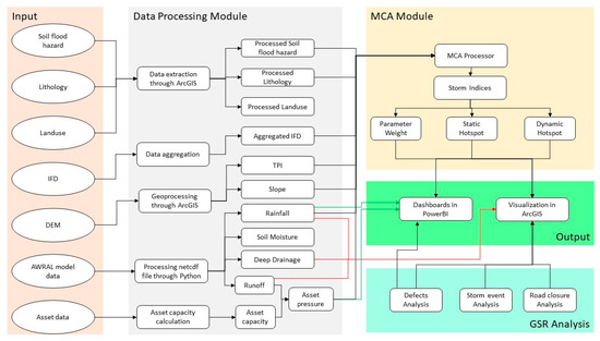
Figure 1.
A Conceptual Framework.
3.1. Data Acquisition, Assimilation, and Integration
Data sources. Various data sources were explored, acquired and assimilated. In particular, stormwater management and asset management data were obtained from Main Roads Western Australia (MRWA) (https://www.mainroads.wa.gov.au/, accessed on 20 December 2022). These included asset inventory data of stormwater drainage and capacity (i.e., culverts, state road network, floodway). We also collected publicly available data in relation to hydro-informatics from several sources, including the Bureau of Meteorology (BoM) (http://www.bom.gov.au/, accessed on 20 December 2022), Shuttle Radar Topography Mission (SRTM) (https://dwtkns.com/srtm30m/, accessed on 20 December 2022), and Landgate (https://www0.landgate.wa.gov.au/, accessed on 20 December 2022). Data from BoM included precipitation, soil moisture, surface runoff, slope of land surface, streamflow, topographic, vegetation, deep drainage, and intensity frequency duration. The data collected from Landgate included state-wide flood records. Lastly, data collected from SRTM included the elevation.
The Australian Landscape Water Balance model (AWRA-L) is a high-resolution (5 km × 5 km) hydrological model developed by the Commonwealth Scientific and Industrial Research Organisation (CSIRO), in collaboration with the BoM and other partners. It estimates the water balance components, such as precipitation, evapotranspiration, soil moisture, and runoff, at a daily time step for the entire Australian continent. The model incorporates a range of datasets, including satellite and radar data, ground-based measurements, and hydrological modelling. The collection of spatial data was processed and handled in Geographic Information Systems (GIS) through ArcGIS (https://www.arcgis.com/index.html, accessed on 20 December 2022) to illustrate the geographical data of the case study area.
Data Processing and Preparation: Slope, topographic wetness index (TWI) and topographic position index (TPI) were derived from DEM. These DEM Derivatives were calculated using ArcGIS Pro and the calculation was automated in Model Builder. Figure 2 shows the final workflow of the model builder. Slope was calculated using an inbuilt tool called “slope” in the geoprocessing toolbox.
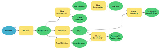
Figure 2.
Workflow from model builder in ArcGIS Pro v3.0.1.
TPI was calculated from the focal statistic and raster calculator [64]. TPI is the difference in elevation at the central point () and the mean elevation across the central point within the local window () (Equation (1)). Furthermore, raster statistics were used to calculate the TPI value using Equation (2) [64]. Mean elevation across the central point within the local window () was calculated using focal statistics. is the elevation value of ith cell and n is the total number of surrounding points employed in the evaluation. The final result produces a tiff file for each pixel showing the topographic position index of that location.
TWI was calculated using the raster calculator in ArcGIS Pro. by applying the following formula in Equation (3) [81]. The final result produces a tiff file for each pixel showing the topographic wetness index of that location. is a specific area and slope angle measured in degree (β) from elevation.
3.2. Pressure on Assets
Pressure on assets was analysed by comparing the capacity of the asset with the runoff received by the asset. Asset capacity was calculated using the dimensions of assets, such as length, radius, height, and slope of culvert or floodway. The flow of water was calculated using the runoff parameters from the AWRAL model. This was used to compare with the capacity of assets. Finally, the pressure was calculated in percentage.
Culvert Capacity: To calculate the capacity (Q) of the culvert, manning’s formula was used (Manning 1891). Equation (4) was used to calculate culvert capacity. Manning’s coefficient value (n) was obtained using Table 3 for every corresponding type of material in the floodway. Values for flow area (A), wetted perimeter (P), and channel slope (S) were obtained from the dimension data of the culvert.
Table 3.
Manning’s coefficient value for different types of material used in construction.
In Equation (5), a simplified method was used to calculate the floodway capacity. Here, is the height of water and L is the length of the floodway. Floodway capacity was calculated using the length of the floodway and assuming the height of 0.3 m.
Furthermore, the catchment data and runoff from AWRA-L model were used to obtain the flow of water at that particular location on the culvert and floodway. The flow of water at the asset’s location and the capacity of the asset were compared to calculate the pressure on the asset in percentage terms.
3.3. Develop Risk Hotspots through a Probabilistic Approach
The factors that could cause the floods were also the factors that could lead to a higher flow of water in asset locations. These parameters were considered for the assessment of hotspots that have a high risk of damage to these assets. The risk is calculated from the hazard and vulnerability following the methodology from [63] using Equation (6). In this study, hazard was the probability of water accumulation conditions calculated through elevation, land use, soil, and factors that affect water flow and accumulation. Similarly, vulnerability was the probability of damage to the assets calculated from the assets receiving high pressure.
The calculation methodology for hazard and vulnerability used in this study is as follows:
Hazard: Hazard referred to the physical parameters that contribute to the potential damage of an asset. In this study, the hazard was calculated based on morphometric and hydrometeorological parameters, which are sourced from various data portals. These parameters included slope, elevation, catchment area, average rainfall intensity, and rainfall duration. To calculate the hazard, the following steps were followed: (i) derived the morphometric parameters, such as slope, elevation, and catchment area, using SRTM data; (ii) obtained the hydrometeorological parameters, such as average rainfall intensity and rainfall duration, from the BoM data, and; (iii) calculated the hazard by combining the morphometric and hydrometeorological parameters using a weighting factor. The weighting factor was derived from AHP analysis, which involved stakeholder input to assess the relative importance of each parameter.
Vulnerability: Vulnerability referred to the susceptibility of an asset to damage from flood events. In this study, the vulnerability was calculated based on the asset pressure, which was the ratio of the water flow (inundation status) in the location of the asset to the capacity of the asset. To calculate the vulnerability, the following steps were followed; (i) obtained the water flow data (inundation status) from the Australian Landscape Water Balance model (AWRA-L) dataset; (ii) determined the capacity of the asset based on asset inventory data regarding stormwater drainage and capacity obtained from MRWA; (iii) calculated the asset pressure by dividing the water flow in the location of the asset by the asset capacity, and; (iv) calculated the vulnerability by normalising the asset pressure value using a sigmoid function, which maps the pressure values across a range between 0 and 1. The sigmoid function was used to model the nonlinear relationship between the asset pressure and the vulnerability. By combining the hazard and vulnerability calculations, a risk map was generated that identified the high-risk hotspots for asset damage from flooding.
Level 1 multi-criteria analysis: The MCA approach was used to create thematic layers of various contributing parameters to generate the risk hotspot map. These parameters for hazard calculation included elevation, slope, aspect, curvature of land, land use, runoff, rainfall, aquifer, and streamflow. Similarly, vulnerability was calculated using asset pressure. This method was the Level 1 option for choosing the parameters based on criteria. In Level 2, the analytical hierarchy process was used for assigning relative importance weight to every parameter. This weight was obtained by creating a pairwise comparison matrix [63]. This matrix was flexible because of its amenability and consideration of the interest of stakeholders by allowing them to input their views and experiences [63].
Level 2 analytical hierarchy process: As mentioned above, this process generated a pairwise comparison matrix [82]. Every parameter was listed in the first column and first row. The value of importance was assigned using the Saaty scale [82]. The format for calculating the pairwise comparison matrix is given in Table 4. Higher weight was given to the most important parameters.
Table 4.
Pairwise comparison matrix calculation.
In MCA, stakeholders could provide their inputs to create criteria for parameter selection via a pairwise comparison matrix; known as the analytic hierarchy process (AHP), it is a widely used method for capturing stakeholders’ preferences and priorities. In our study, stakeholders, including government personnel and academics, were asked to evaluate the importance of each criterion or parameter relative to all the other criteria. Stakeholders were presented with a pairwise comparison matrix, which listed all the criteria in rows and columns; they were then asked to indicate the relative importance of each criterion by assigning numerical values that reflected the strength of the relationship between the criteria.
The numerical values typically ranged from 1 (indicating equal importance) to 9 (indicating very strong importance). The values could also be fractional, such as 1/3, 1/5, etc.; fractional values indicated intermediate levels of importance. Once stakeholders had completed the pairwise comparison matrix, the data were analysed to derive weights for each criterion. These weights reflected the relative importance of each criterion in the decision-making process and were used to weigh the scores of each option in the MCA.
Further estimated eigenvalue () was calculated using Equation (7) [63]. can be the value for row 1 of the pairwise comparison matrix. Similarly, value can be calculated for every row in the pairwise comparison matrix termed as .
Here, each element of the row is denoted by the values of . Furthermore, relative importance weight () was calculated using all eigenvalues in pairwise comparison matrix. Equation (8) is used to calculate relative importance weight of each row in the pairwise comparison matrix [63]
This matrix was checked for consistency using consistency ratio (). Consistency ratio is calculated from relative consistency index () and consistency index (), as shown in Equation (9). The relative consistency index depends on the number of parameters (as shown in Table 5) for n = 1, 2 … 8 (adapted from [82]).
Table 5.
Random consistency index (RI).
The consistency index was calculated using Equation (10) [63]. Here is calculated by summing up the product of RIW and the sum of every column representing the criteria. This is shown in the right most column of Table 4.
A consistency ratio of less than 0.1 shows consistent importance is assigned to the parameters in the respective pairwise comparison matrix.
Level 3 data classification and weighting: Data for every parameter consisted of unique values or numerical ranges. For example, the lithology parameter’s data was in .shp format (Shapefile). It had a unique value depending on whether rock’s classification as sedimentary, metasedimentary, metamorphic, metai, or igneous; this classification was represented by a polygon. Each different type of rock had a different impact on the water flow. Contrastingly, the data of elevation was in .tif format (image file). The values were all numbers ranging from 58 to 864 m. Different elevations all had a different impact on flow of water.
To incorporate this variation into the final hotspot, a pairwise comparison matrix was generated for every parameter. RIW is calculated for every range, while the consistency of that pairwise comparison matrix was confirmed using CI. Steps in level 2 and level 3 were repeated to calculate the vulnerability, using the asset pressure data to generate accurate results. Hazard and vulnerability were calculated using the following equation:
Risk hotspot map: A raster image was generated for each parameter using the original data and relative importance weight. Data was imported into ArcGIS software v.10.8.2. Table 6 shows the source, type of data, and process for each parameter.
Table 6.
Multi-criteria analysis parameters processing.
A shapefile of a 50 m road buffer was generated using a buffer tool. We clipped the data using the road buffer shapefile, reducing the processing time by only focusing on the required area. The clipped data were assigned relative importance weight using the results calculated from the pairwise comparison matrix. Using summary statistics, new hazard layer and vulnerability layer data were generated from all parameter raster layers. The final raster data were converted to vector data to make a hotspot map.
3.4. Validation of Hotspot
The risk map was generated using the vulnerability data from 2020; hence, the road closure that occurred in 2020 was screened from the road closure map in Figure 3. The road closure and risk for 2020 can be observed in Figure 3. To understand the temporal behaviour of risk hotspots, the time series analysis of risk and road closure was performed. Figure 3 shows the maps of road closure and risk from January to June 2020. The large size map for all size months can be observed from Figure 4, Figure 5, Figure 6, Figure 7, Figure 8 and Figure 9. High risk and road closure was identified for Kimberley region, and southern areas of the Mid West-Gascoyne regions. High density of risk spots could be clearly observed around the road closure. However, the road closure in north Kimberley was observed to be persistent for long time duration. Road closure in Mid West-Gascoyne, and high-risk spots, were identified in January 2020 and February 2020.
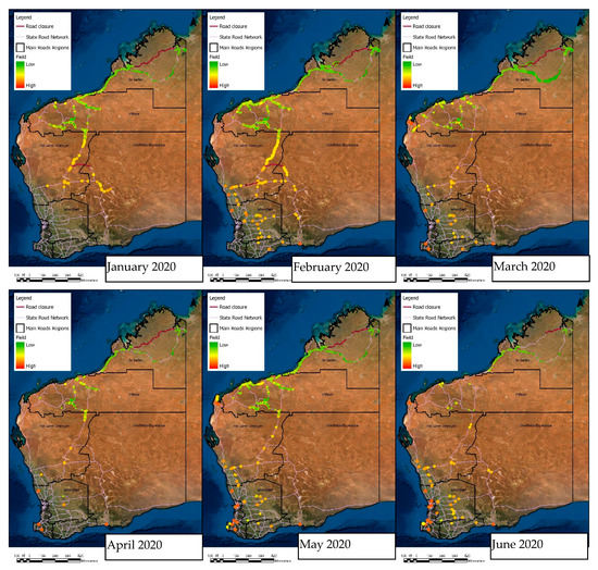
Figure 3.
Time series map of risk and road closure from January to June 2020.
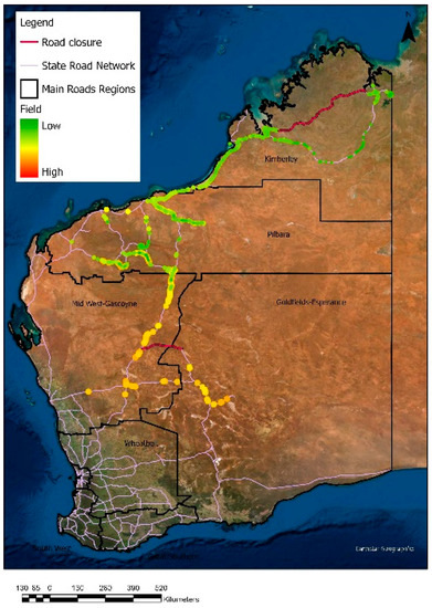
Figure 4.
Risk and road closure in January 2020.
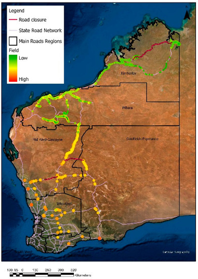
Figure 5.
Risk and road closure in February 2020.
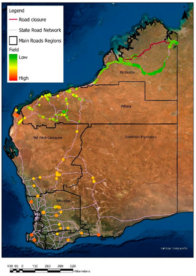
Figure 6.
Risk and road closure in March 2020.
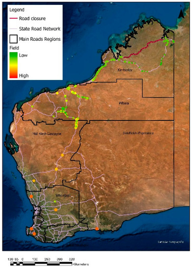
Figure 7.
Risk and road closure in April 2020.
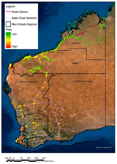
Figure 8.
Risk and road closure in May 2020.
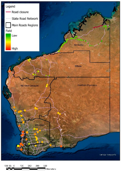
Figure 9.
Risk and road closure in June 2020.
Road closures were a useful metric for verifying the identified hotspots of high risk for asset damage in the study because they are a direct consequence of flooding and can be easily tracked and verified. When a road was closed due to flooding, it was an indication that the floodwater had exceeded the capacity of the stormwater drainage system, leading to the flooding of the road and potential damage to the surrounding assets. Thus, road closures could serve as a reliable proxy for identifying areas of potential asset damage due to flooding. By comparing the identified hotspots with road closures, this study helped to verify the accuracy of the risk maps and provided evidence of the effectiveness of the data-driven approach. If the identified hotspots aligned with areas that experience road closures due to flooding, it provided strong evidence that the risk maps are reliable and could be used to prioritise asset management interventions. On the other hand, if there was a mismatch between the identified hotspots and areas of road closure, it may suggest that there were other factors at play for which the model failed to account, or that the model itself needs to be refined.
4. Results and Discussion
4.1. Data Acquisition
To validate the utility of the proposed approach, a case study was been carried out in Western Australia (WA) state. WA is the largest state in Australia, spanning for around 2.5 million square kilometres. Figure 10 includes the regional map of WA.
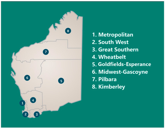
Figure 10.
Regional map of Western Australia [83].
Maps for required parameters were generated from data collection, assimilation, and integration. Figure 11 shows the elevation map of Western Australia. Elevation in Western Australia ranges from 66.8 to 1247 m. Higher elevation is observed inland, decreasing gradually towards the coastal area. Moreover, in northern Western Australia, a high peak can be observed. Figure 12 shows the map of the slope of terrain across Western Australia. Slope varies between 0 to 75.3. Slope can be observed as high in north, north-west and southwestern parts of Western Australia, with the elevation map showing stiff parches of land in these areas. The topographic position index shows the presence of a valley or ridge in the terrain. From Figure 13, it can be observed that regions with varying slope values also have a higher variation in TPI values. TWI is found to be constantly varying across study regions, with higher TWI values recorded in inland regions (as depicted in Figure 14). An Inverse relationship between TWI and slope is found. The flat regions are found to have higher TWI values than can be observed from Figure 12 and Figure 13.
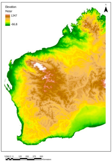
Figure 11.
Elevation map of Western Australia.
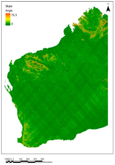
Figure 12.
Map of terrain slope of Western Australia.
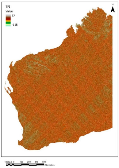
Figure 13.
Topographic position index map of Western Australia.
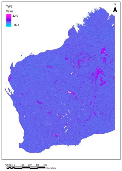
Figure 14.
Topographic wetness index map of Western Australia.
The road closure data was obtained from the Main Roads data portal. The data available dates from after 1996. Figure 15 shows the road closure stretch on the state road network. Frequent road closures can be observed in Kimberley, Pilbara, Mid West-Gascoyne, and Goldfields-Esperance. No road closure was observed in the South West region, while road closures were rare in the Wheatbelt and Great Southern region.
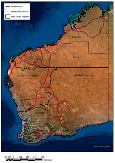
Figure 15.
Road closure due to rain events.
Intensity Frequency duration: BoM provides the design rainfall data in the form of intensity frequency duration; results ranged from a very frequent probability of 12 exceedances per yar (EY) to 0.2 EY, frequent and infrequent probability of 1 EY to 1% Annual Exceedance Probability (AEP), and rare probability of 1-in-100 AEP to 1-in-2000 AEP. Figure 16 illustrates both intensity frequency duration and asset capacity. The graph shows frequency duration with respect to intensity in unit of mm per hours. It can be observed that lower intensity and same intensity both cause frequent exceedance when such rainfall happens in smaller time duration (1 h), compared to the same intensity in a longer time period (24 h).
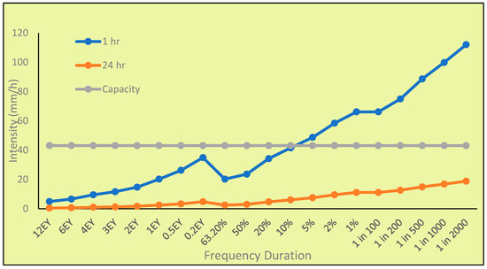
Figure 16.
Illustration of intensity frequency duration and asset capacity.
4.2. Pressure on Assets
Percentage pressure on culverts and floodways in 2020 can be seen in Figure 17 and Figure 18, respectively. It can be observed that culverts received higher pressure compared to the floodways. Culverts received higher pressure in Kimberley and the southwestern region, while floodway pressure was highest in the northern region.
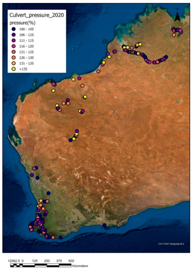
Figure 17.
Pressure on culverts.
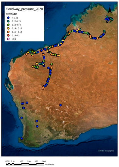
Figure 18.
Pressure on Floodways.
4.3. Multi-Criteria Analysis
The pairwise comparison matrix for all parameters can be seen in Table 7. It can be observed that IFD received the highest weight, followed by slope, elevation, and TPI. In contrast, lithology, land use, and TWI received lower relative importance based on their impact on the behaviour of water, such as flow, infiltration, evapotranspiration, and accumulation.
Table 7.
Pairwise comparison matrix results.
Furthermore, this pairwise consistency matrix was checked for consistency using a consistency ratio. Here, a consistency ratio of 0.03 was observed; as that ratio is less than 0.1, this pairwise comparison matrix can be said to have consistent weighting.
Relative importance weights for all parameters were produced using a pairwise comparison matrix. The resultant RIW for various classes or types of data is shown in Table 8. The consistency ratio of the pairwise comparison matrix was found to be less than 0.1 for consistency. Similarly, for the vulnerability map, the pressure on culvert and floodway was used. Table 9 shows the relative importance weight of different pressure ranges calculated from the pairwise comparison matrix. It is also important to note that the factors do not cause multicollinearity due to the independency between factors and their low correlation.
Table 8.
Relative importance weight and consistency ratio for unique values and range of data.
Table 9.
Relative importance weight and consistency ratio for range pressure of assets.
4.4. Hazard Vulnerability
Relative importance weights from Table 8 and Table 9 were used to reclassify every parameter. New values were assigned by converting the original value to the allocated weight. The reclassified raster images were then multiplied by the relative importance weight of respective parameters given in Table 9. Figure 19 shows the hazard map generated from parameters in Table 9 including Land use, lithology, soil hazard, IFD, elevation, slope, TPI, and TWI. A higher level of hazard is observed along the coastline of Western Australia. From the map of elevation in Figure 11, it can be observed that lower elevation is found along the coastline. It can be also observed that there is an inverse relation of elevation with the hazard level.
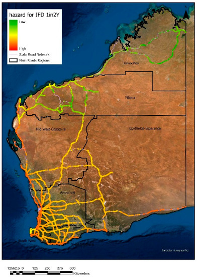
Figure 19.
Map of flood hazard.
The map in Figure 20 shows the vulnerability which was generated from the reclassified value of pressure on culverts and floodways in 2020. A high vulnerability level can be observed to have a direct relation to the topographic position index (Figure 13).
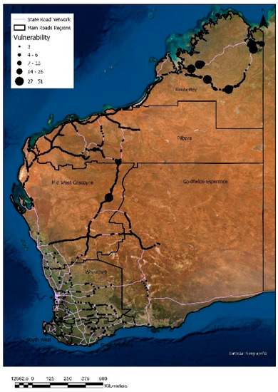
Figure 20.
Map of the vulnerability of assets to damage.
Overall, a higher level of hazard can be observed in the south of Western Australia compared to north regions, such as including Pilbara and Kimberley. On the other hand, high vulnerability spots can be seen in the Kimberley and northern Midwest-Gascoyne regions. Despite major differences, the presence of vulnerability and high levels of hazard can be observed along the western cost and the south west region. It can be noted that regions with a high level of hazard may not have a higher level of vulnerability [63].
Risk map: In this study, the variation in risk across the Western Australia in 2020 was measured. Hazard map and vulnerability in 2020 were merged to visualise the risk map (Figure 21). The resultant map shows the asset damage risk level in 2020. High-risk areas can be observed in Kimberley, the north-west road stretch of Midwest-Gascoyne region, and the South west region.
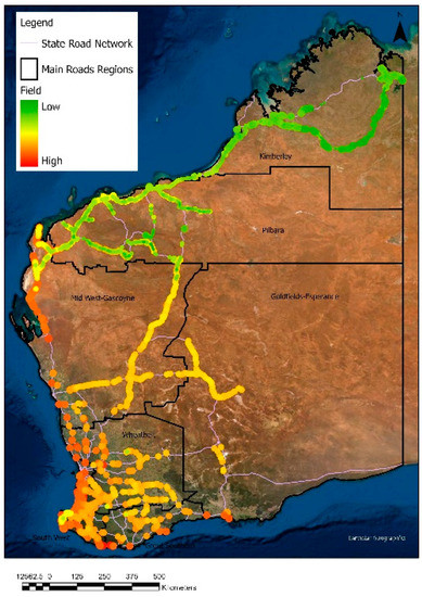
Figure 21.
Map of risk hotspots for asset damage.
Note that the differences in data points and lines, known as mapping scale, are shown in the figures above.
Sensitivity analysis in MCA has been performed using different techniques, such as varying the weights of the criteria within a specified range, or examining the impact of varying weights on the ranking of the alternatives. This has helped us to identify the range of values for the weights of each factor, producing the most stable and reliable rankings of the alternatives. Furthermore, the authors found the consistency ratio for the pairwise comparison matrix to be less than 0.1, which is considered an acceptable level of consistency. This indicates that the judgments made by the decision makers in the pairwise comparison process were reasonably consistent. Moreover, we incorporated a well-established method for deriving the pairwise comparison matrix, and followed standard procedures to ensure consistency and validity. This can increase the reliability and robustness of the results.
5. Discussion and Limitations
The multi-criteria analysis (MCA) technique is a powerful decision making tool that can be used to assess and compare multiple criteria or factors that may influence a particular decision. When MCA is combined with Geographic Information System (GIS) technology, it can enhance decision making processes by incorporating spatial data, analysing spatial relationships and patterns, and visualising the results on maps. Incorporating MCA techniques provide several benefits to regional governments in Australia in terms of preparations for and mitigations during future flood events. MCA can help regional governments make informed decisions by evaluating the different criteria that are relevant to flood preparedness and mitigation. Benefits of using MCA for flood preparedness and mitigation include: (i) identifying and prioritising critical criteria: MCA can help regional governments identify and prioritise the criteria that are most important for flood preparedness and mitigation. This can help to ensure that resources are allocated to the most critical areas, and that the most effective strategies are implemented to address flood risks; (ii) evaluating trade-offs: MCA can help regional governments evaluate the trade-offs between different strategies and criteria. For example, governments can use MCA to evaluate the trade-offs between the costs of flood mitigation strategies and the potential benefits in terms of reducing the impact of floods; (iii) incorporating stakeholder input: MCA can help regional governments incorporate stakeholder input into the decision making process. By involving stakeholders in the development of criteria and the evaluation of strategies, regional governments can ensure that the decision making process is transparent and reflects the interests and concerns of all stakeholders; (iv) supporting data-driven decision making: MCA can help regional governments make data-driven decisions by providing a structured approach to evaluating criteria and strategies. This can help to ensure that decisions are based on objective criteria and data, rather than subjective opinions or biases, and; (v) enhancing communication and transparency: MCA can help to enhance communication and transparency by providing a clear and structured approach to evaluating flood preparedness and mitigation strategies. This can help to build trust and credibility with stakeholders, and improve public understanding of and support for flood preparedness and mitigation efforts.
This paper aims to identify regions that are likely vulnerable to a higher risk of damage to their assets. In the provided case study, we indicate valuable insights into the flood-related parameters in Western Australia that can increase the risk of damage to road and stormwater management assets in 2020. The findings of this study also provide the relationship between parameters and the risk. To sum up, the following are the outcomes of the study:
The topographic index has a relationship to the vulnerability of assets to damage. The presence of ridges and valleys might cause water accumulation.
Intensity frequency duration of design rainfall studies revealed higher pressure on the assets when there is rain in a small duration of time compared to rain in a longer duration. Culverts receive significantly higher pressure compared to the floodways.
The hazard distribution was found to be related to elevation. According to this study lower elevations regions were found to have a higher level of hazard.
Regions with high vulnerability might not have a higher level of hazard.
A high number of road closures and risk spots were found in January 2020 and February 2020. However, parameters were observed at a low level in March–June 2020. The road closure stretch may not align with the hotspot map because of the nature of the risk map.
The focus on damage to roads in the context of flood risk and asset management is due to the critical role that roads play in maintaining access and mobility in urban and rural areas. When roads are damaged or closed due to flooding, it can severely impact the ability of people and goods to move, resulting in economic and social disruptions. Moreover, damage to roads can also have safety implications, such as increased risk of accidents due to damaged road surfaces, or reduced visibility in flooded areas. Roads are also often the most visible and easily quantifiable asset in the floodplain; as a result, they can serve as an important indicator of the potential impacts of flooding on other assets and infrastructure in the area. By focusing on damage to roads, asset managers can prioritise interventions that help reduce the risk of road damage and closure, which can in turn mitigate the impact of flooding on other assets, such as buildings and farmland. In addition, damage to roads can be expensive to repair and have a significant impact on local and regional economies. By focusing on reducing the risk of road damage, asset managers can help minimise the economic impact of flooding events and promote faster recovery in affected areas.
The limitations of this study include the computation capacity; if the hotspot map is generated without limiting it to asset location, this can also provide a stretch of road where there is higher risk. However, because of the limitation of intensity frequency duration data, the assessment calculation is limited to the asset location. Furthermore, studying the state-wise risk distribution can give more insights into the asset management system. Multi-criteria analysis can incorporate the rainfall and a greater number of DEM derivatives that are linked to the flow and accumulation of water. This study could also be improved by adding parameters, such as the road traffic and vegetation in the region, from satellite sources, such as NDVI from Landgate. Road traffic also places stress on the road and alters the strength of the road. Similarly, the presence of vegetation prevents the build-up of fast-moving water that can create the conditions required for flash flooding and increase the risks posed to the stormwater management system.
6. Conclusions
Floodwater is a destructive phenomenon that causes substantial damage to road assets and infrastructure. Sustainable flood management focusing on prevention, protection, and preparedness is the focus of this paper. Sustainable flood management would help government agencies to effectively respond to extreme climate conditions and their impacts by enabling more efficient asset management strategies. The proposed approach serves as a useful tool for government agencies in Western Australia to effectively manage and mitigate the risks associated with flood events. By combining hazard and vulnerability analysis using MCA, the approach offers a comprehensive view of the factors affecting the risk of asset damage and can help prioritise efforts and resources in the most vulnerable areas. With the increasing influence of climate change on extreme weather events, this approach can provide important insights for data-driven asset management, and the development of more accurate flood models and early warning systems.
The data used in this study were collected from various data sources. In particular, rainfall and runoff data were obtained from Australian Water Resources Assessment Landscape (AWRA-L) model. Stormwater management and asset management data were obtained from Main Roads WA. These include asset inventory data of stormwater drainage and capacity. Publicly available data in relation to hydro-informatics were collected from BoM, SRTM, and Landgate. MCA was then used to define the high-risk hotspots for asset damage. These state-wide hotspots were validated using road closure data from Main Roads WA. Road damage risk maps were generated using hazard and vulnerability raster maps. Road damage hazard was calculated from morphometric and hydrometeorological parameters sourced from various data portals. Vulnerability was calculated based on pressure on assets. The hotspot analysis shows high risk can be observed in Kimberley, the north-west road stretch in the Midwest-Gascoyne region, and the South West region. Moreover, after validation with the road closure data. High flooding risk and road closures can be observed in Kimberley region and south of Mid WestGascoyne region. The time series analysis is undertaken in order to understand the temporal variation in risk map. Alignment in the occurrence of risk spots and road closure is observed. However, further work on multiple years could help understand risk distribution more accurately.
Author Contributions
Conceptualization, P.W. and H.P.; Methodology, P.W., J.H. and H.P.; Software, P.W., B.A.-S. and H.P.; Validation, P.W., B.A.-S. and H.P.; Formal analysis, B.A.-S.; Investigation, B.A.-S. and J.H.; Resources, P.W. and K.S.; Writing—original draft, H.P.; Writing—review & editing, B.A.-S. and K.S.; Visualization, B.A.-S. and J.H.; Supervision, P.W. and K.S.; Project administration, K.S. All authors have read and agreed to the published version of the manuscript.
Funding
This research received no external funding.
Institutional Review Board Statement
Not applicable.
Informed Consent Statement
Not applicable.
Data Availability Statement
The data presented in this study are available on request from the corresponding author.
Conflicts of Interest
The authors declare no conflict of interest.
References
- Liu, J.; Zhang, Y.; Yang, Y.; Gu, X.; Xiao, M. Investigating relationships between Australian flooding and large-scale climate indices and possible mechanism. J. Geophys. Res. Atmos. 2018, 123, 8708–8723. [Google Scholar] [CrossRef]
- Berland, A.; Shiflett, S.A.; Shuster, W.D.; Garmestani, A.S.; Goddard, H.C.; Herrmann, D.L.; Hopton, M.E. The role of trees in urban stormwater management. Landsc. Urban Plan. 2017, 162, 167–177. [Google Scholar] [CrossRef] [PubMed]
- Khayan, K.; Husodo, A.H.; Astuti, I.; Sudarmadji, S.; Djohan, T.S. Rainwater as a source of drinking water: Health impacts and rainwater treatment. J. Environ. Public Health 2019, 2019, 1760950. [Google Scholar] [CrossRef] [PubMed]
- Newhart, K.B.; Holloway, R.W.; Hering, A.S.; Cath, T.Y. Data-driven performance analyses of wastewater treatment plants: A review. Water Res. 2019, 157, 498–513. [Google Scholar] [CrossRef] [PubMed]
- Matheswaran, K.; Alahacoon, N.; Pandey, R.; Amarnath, G. Flood risk assessment in South Asia to prioritize flood index insurance applications in Bihar, India. Geomat. Nat. Hazards Risk 2019, 10, 26–48. [Google Scholar] [CrossRef]
- Pallathadka, A.; Sauer, J.; Chang, H.; Grimm, N.B. Urban flood risk and green infrastructure: Who is exposed to risk and who benefits from investment? A case study of three US Cities. Landsc. Urban Plan. 2022, 223, 104417. [Google Scholar] [CrossRef]
- Molinari, D.; De Bruijn, K.M.; Castillo-Rodríguez, J.T.; Aronica, G.T.; Bouwer, L.M. Validation of flood risk models: Current practice and possible improvements. Int. J. Disaster Risk Reduct. 2019, 33, 441–448. [Google Scholar] [CrossRef]
- Scaini, A.; Stritih, A.; Brouillet, C.; Scaini, C. Flood risk and river conservation: Mapping citizen perception to support sustainable river management. Front. Earth Sci. 2021, 9, 510. [Google Scholar] [CrossRef]
- Abu-Salih, B.; Wongthongtham, P.; Zhu, D.; Chan, K.Y.; Rudra, A.; Abu-Salih, B.; Wongthongtham, P.; Zhu, D.; Chan, K.Y.; Rudra, A. Predictive analytics using Social Big Data and machine learning. In Social Big Data Analytics: Practices, Techniques, and Applications; Springer: Singapore, 2021; pp. 113–143. [Google Scholar]
- Hawchar, L.; Naughton, O.; Nolan, P.; Stewart, M.G.; Ryan, P.C. A GIS-based framework for high-level climate change risk assessment of critical infrastructure. Clim. Risk Manag. 2020, 29, 100235. [Google Scholar] [CrossRef]
- Kumar, N.; Poonia, V.; Gupta, B.B.; Goyal, M.K. A novel framework for risk assessment and resilience of critical infrastructure towards climate change. Technol. Forecast. Soc. Chang. 2021, 165, 120532. [Google Scholar] [CrossRef]
- Pathak, S.; Liu, M.; Jato-Espino, D.; Zevenbergen, C. Social, economic and environmental assessment of urban sub-catchment flood risks using a multi-criteria approach: A case study in Mumbai City, India. J. Hydrol. 2020, 591, 125216. [Google Scholar] [CrossRef]
- Brimfield, B.E.; Myers, S.D. An integrated approach to benefits realisation of railway condition monitoring innovations. In Proceedings of the 5th IET Conference on Railway Condition Monitoring and Non-Destructive Testing (RCM 2011), Derby, UK, 29–30 November 2011. [Google Scholar]
- Li, Q.; Kumar, A. National & International Practices in Decision Support Tools in Road Asset Management; CRC for Construction Innovation: Brisbane, QLD, Australia, 2003. [Google Scholar]
- Christodoulou, S.; Deligianni, A. A neurofuzzy decision framework for the management of water distribution networks. Water Resour. Manag. 2010, 24, 139–156. [Google Scholar] [CrossRef]
- Sobieraj, J.; Bryx, M.; Metelski, D. Stormwater Management in the City of Warsaw: A Review and Evaluation of Technical Solutions and Strategies to Improve the Capacity of the Combined Sewer System. Water 2022, 14, 2109. [Google Scholar] [CrossRef]
- Hafeez, F.; Frost, A.; Vaze, J.; Dutta, D.; Smith, A.; Elmahdi, A. A new integrated continental hydrological simulation system. Water J. Aust. Water Assoc. 2015, 42, 75–82. [Google Scholar]
- Viney, N.; Vaze, J.; Crosbie, R.; Wang, B.; Dawes, W.; Frost, A. AWRA-L v5.0: Technical Description of Model Algorithms and Inputs; CSIRO: Perth, SA, Australia, 2015. [Google Scholar] [CrossRef]
- Elmahdi, A.; Hafeez, M.; Smith, A.; Frost, A.; Vaze, J.; Dutta, D. Australian Water Resources Assessment Modelling System (AWRAMS)-informing water resources assessment and national water accounting. In Proceedings of the 36th Hydrology and Water Resources Symposium: The Art and Science of Water, Hobart, TAS, Australia, 7–10 December 2015; Engineers Australia: Barton, CBR, Australia, 2015; p. 979. [Google Scholar]
- Frost, A.J.; Ramchurn, A.; Hafeez, M. Evaluation of the Bureau’s Operational AWRA-L Model; Bureau of Meteorology: Melbourne, VIC, Australia, 2016; p. 80.
- Raupach, M.R.; Briggs, P.R.; Haverd, V.; King, E.A.; Paget, M.; Trudinger, C.M. Australian Water Availability Project (AWAP): CSIRO Marine and Atmospheric Research Component: Final Report for Phase 3; Centre for Australian Weather and Climate Research (Bureau of Meteorology and CSIRO): Melbourne, VIC, Australia, 2009; p. 67.
- Wang, Y.P.; Kowalczyk, E.; Leuning, R.; Abramowitz, G.; Raupach, M.R.; Pak, B.; van Gorsel, E.; Luhar, A. Diagnosing errors in a land surface model (CABLE) in the time and frequency domains. J. Geophys. Res. Biogeosci. 2011, 116, G01034. [Google Scholar] [CrossRef]
- Kowalczyk, E.A.; Wang, Y.P.; Law, R.M.; Davies, H.L.; McGregor, J.L.; Abramowitz, G. The CSIRO Atmosphere Biosphere Land Exchange (CABLE) model for use in climate models and as an offline model. CSIRO Mar. Atmos. Res. Pap. 2006, 13, 42. [Google Scholar]
- Mosavi, A.; Ozturk, P.; Chau, K.-W. Flood prediction using machine learning models: Literature review. Water 2018, 10, 1536. [Google Scholar] [CrossRef]
- Van den Honert, R.C.; McAneney, J. The 2011 Brisbane floods: Causes, impacts and implications. Water 2011, 3, 1149–1173. [Google Scholar] [CrossRef]
- Shrestha, D.L.; Robertson, D.E.; Wang, Q.J.; Pagano, T.C.; Hapuarachchi, H.A. Evaluation of numerical weather prediction model precipitation forecasts for short-term streamflow forecasting purpose. Hydrol. Earth Syst. Sci. 2013, 17, 1913–1931. [Google Scholar] [CrossRef]
- Daley, R. Atmospheric Data Analysis; Cambridge University Press: Cambridge, UK, 1993. [Google Scholar]
- Echeverribar, I.; Morales-Hernández, M.; Brufau, P.; García-Navarro, P. 2D numerical simulation of unsteady flows for large scale floods prediction in real time. Adv. Water Resour. 2019, 134, 103444. [Google Scholar] [CrossRef]
- Yoon, S.-S. Adaptive blending method of radar-based and numerical weather prediction QPFs for urban flood forecasting. Remote Sens. 2019, 11, 642. [Google Scholar] [CrossRef]
- Kundzewicz, Z.W.; Pińskwar, I.; Brakenridge, G.R. Changes in river flood hazard in Europe: A review. Hydrol. Res. 2018, 49, 294–302. [Google Scholar] [CrossRef]
- Shakirah, J.A.; Sidek, L.M.; Hidayah, B.; Nazirul, M.Z.; Jajarmizadeh, M.; Ros, F.C.; Roseli, Z.A. A review on flood events for kelantan river watershed in malaysia for last decade (2001–2010). IOP Conf. Ser. Earth Environ. Sci. 2016, 32, 012070. [Google Scholar] [CrossRef]
- Kenley, R.; Harfield, T.; Bedggood, J. Road asset management: The role of location in mitigating extreme flood maintenance. Procedia Econ. Financ. 2014, 18, 198–205. [Google Scholar] [CrossRef]
- Kim, B.; Sanders, B.F.; Han, K.; Kim, Y.; Famiglietti, J.S. Calibration of stormwater management model using flood extent data. In Proceedings of the Institution of Civil Engineers-Water Management; Thomas Telford Ltd.: London, UK, 2014; pp. 17–29. [Google Scholar]
- Beecroft, A.; Peters, E.; Toole, T. Life-cycle costing of rain and flood events in Queensland—Case studies and network-wide implications. Road Transp. Res. J. Aust. New Zealand Res. Pract. 2017, 26, 22–35. [Google Scholar]
- Costabile, P.; Costanzo, C.; Macchione, F. Comparative analysis of overland flow models using finite volume schemes. J. Hydroinform. 2012, 14, 122–135. [Google Scholar] [CrossRef]
- Lee, T.H.; Georgakakos, K.P. Operational Rainfall Prediction on Meso-γ Scales for Hydrologic Applications. Water Resour. Res. 1996, 32, 987–1003. [Google Scholar] [CrossRef]
- Hu, Z.-J.; Wang, L.-L.; Tang, H.-W.; Qi, X.-M. Prediction of the future flood severity in plain river network region based on numerical model: A case study. J. Hydrodyn. Ser. B 2017, 29, 586–595. [Google Scholar] [CrossRef]
- Costabile, P.; Costanzo, C.; Macchione, F. A storm event watershed model for surface runoff based on 2D fully dynamic wave equations. Hydrol. Process. 2013, 27, 554–569. [Google Scholar] [CrossRef]
- Valipour, M.; Banihabib, M.E.; Behbahani, S.M.R. Comparison of the ARMA, ARIMA, and the autoregressive artificial neural network models in forecasting the monthly inflow of Dez dam reservoir. J. Hydrol. 2013, 476, 433–441. [Google Scholar] [CrossRef]
- Elsafi, S.H. Artificial neural networks (ANNs) for flood forecasting at Dongola Station in the River Nile, Sudan. Alex. Eng. J. 2014, 53, 655–662. [Google Scholar] [CrossRef]
- Deo, R.C.; Şahin, M. Application of the artificial neural network model for prediction of monthly standardized precipitation and evapotranspiration index using hydrometeorological parameters and climate indices in eastern Australia. Atmos. Res. 2015, 161, 65–81. [Google Scholar] [CrossRef]
- Ramana, R.V.; Krishna, B.; Kumar, S.R.; Pandey, N.G. Monthly rainfall prediction using wavelet neural network analysis. Water Resour. Manag. 2013, 27, 3697–3711. [Google Scholar] [CrossRef]
- Shamim, M.A.; Hassan, M.; Ahmad, S.; Zeeshan, M. A comparison of artificial neural networks (ANN) and local linear regression (LLR) techniques for predicting monthly reservoir levels. KSCE J. Civ. Eng. 2016, 20, 971–977. [Google Scholar] [CrossRef]
- Araghinejad, S.; Azmi, M.; Kholghi, M. Application of artificial neural network ensembles in probabilistic hydrological forecasting. J. Hydrol. 2011, 407, 94–104. [Google Scholar] [CrossRef]
- Cunningham, S.C.; Griffioen, P.; White, M.D.; Nally, R.M. Assessment of ecosystems: A system for rigorous and rapid mapping of floodplain forest condition for Australia’s most important river. Land Degrad. Dev. 2018, 29, 127–137. [Google Scholar] [CrossRef]
- Prasad, R.; Deo, R.C.; Li, Y.; Maraseni, T. Input selection and performance optimization of ANN-based streamflow forecasts in the drought-prone Murray Darling Basin region using IIS and MODWT algorithm. Atmos. Res. 2017, 197, 42–63. [Google Scholar] [CrossRef]
- Cannas, B.; Fanni, A.; Sias, G.; Tronci, S.; Zedda, M.K. River flow forecasting using neural networks and wavelet analysis. Geophys. Res. Abstr 2005, 7, 08651. [Google Scholar]
- Tantanee, S.; Patamatammakul, S.; Oki, T.; Sriboonlue, V.; Prempree, T. Coupled wavelet-autoregressive model for annual rainfall prediction. J. Environ. Hydrol. 2005, 13, 1–8. [Google Scholar]
- Mekanik, F.; Imteaz, M.A.; Talei, A. Seasonal rainfall forecasting by adaptive network-based fuzzy inference system (ANFIS) using large scale climate signals. Clim. Dyn. 2016, 46, 3097–3111. [Google Scholar] [CrossRef]
- Kisi, O.; Nia, A.M.; Gosheh, M.G.; Tajabadi, M.R.J.; Ahmadi, A. Intermittent streamflow forecasting by using several data driven techniques. Water Resour. Manag. 2012, 26, 457–474. [Google Scholar] [CrossRef]
- Li, C.; Guo, S.; Zhang, J.; Guo, J. A modified NLPM-ANN model and its application to flood forecasting. Eng. J. Wuhan Univ. 2009, 42, 1–5. [Google Scholar]
- Huang, S.; Chang, J.; Huang, Q.; Chen, Y. Monthly streamflow prediction using modified EMD-based support vector machine. J. Hydrol. 2014, 511, 764–775. [Google Scholar] [CrossRef]
- Bass, B.; Bedient, P. Surrogate modeling of joint flood risk across coastal watersheds. J. Hydrol. 2018, 558, 159–173. [Google Scholar] [CrossRef]
- Tan, Q.-F.; Lei, X.-H.; Wang, X.; Wang, H.; Wen, X.; Ji, Y.; Kang, A.-Q. An adaptive middle and long-term runoff forecast model using EEMD-ANN hybrid approach. J. Hydrol. 2018, 567, 767–780. [Google Scholar] [CrossRef]
- Ravansalar, M.; Rajaee, T.; Kisi, O. Wavelet-linear genetic programming: A new approach for modeling monthly streamflow. J. Hydrol. 2017, 549, 461–475. [Google Scholar] [CrossRef]
- Shafapour Tehrany, M.; Shabani, F.; Jebur, M.N.; Hong, H.; Chen, W.; Xie, X. GIS-based spatial prediction of flood prone areas using standalone frequency ratio, logistic regression, weight of evidence and their ensemble techniques. Geomat. Nat. Hazards Risk 2017, 8, 1538–1561. [Google Scholar] [CrossRef]
- Manfreda, S.; Nardi, F.; Samela, C.; Grimaldi, S.; Taramasso, A.C.; Roth, G.; Sole, A. Investigation on the use of geomorphic approaches for the delineation of flood prone areas. J. Hydrol. 2014, 517, 863–876. [Google Scholar] [CrossRef]
- Papaioannou, G.; Vasiliades, L.; Loukas, A. Multi-criteria analysis framework for potential flood prone areas mapping. Water Resour. Manag. 2015, 29, 399–418. [Google Scholar] [CrossRef]
- Majumder, R.; Bhunia, G.S.; Patra, P.; Mandal, A.C.; Ghosh, D.; Shit, P.K. Assessment of flood hotspot at a village level using GIS-based spatial statistical techniques. Arab. J. Geosci. 2019, 12, 409. [Google Scholar] [CrossRef]
- Aksoy, H.; Kirca, V.S.O.; Burgan, H.I.; Kellecioglu, D. Hydrological and hydraulic models for determination of flood-prone and flood inundation areas. Proc. Int. Assoc. Hydrol. Sci. 2016, 373, 137–141. [Google Scholar] [CrossRef]
- Falguni, M.; Singh, D. Detecting flood prone areas in Harris County: A GIS based analysis. GeoJournal 2020, 85, 647–663. [Google Scholar]
- Pratidina, G.; Santoso, P.B. Detection of satellite data-based flood-prone areas using logistic regression in the central part of Java Island. J. Phys. Conf. Ser. 2019, 1367, 012086. [Google Scholar] [CrossRef]
- Mishra, K.; Sinha, R. Flood risk assessment in the Kosi megafan using multi-criteria decision analysis: A hydro-geomorphic approach. Geomorphology 2020, 350, 106861. [Google Scholar] [CrossRef]
- Rana, V.K.; Suryanarayana, T.M.V. GIS-based multi criteria decision making method to identify potential runoff storage zones within watershed. Ann. GIS 2020, 26, 149–168. [Google Scholar] [CrossRef]
- Rozos, D.; Bathrellos, G.D.; Skillodimou, H.D. Comparison of the implementation of rock engineering system and analytic hierarchy process methods, upon landslide susceptibility mapping, using GIS: A case study from the Eastern Achaia County of Peloponnesus, Greece. Environ. Earth Sci. 2011, 63, 49–63. [Google Scholar] [CrossRef]
- Stefanidis, S.; Stathis, D. Assessment of flood hazard based on natural and anthropogenic factors using analytic hierarchy process (AHP). Nat. Hazards 2013, 68, 569–585. [Google Scholar] [CrossRef]
- Saaty, T.L. A scaling method for priorities in hierarchical structures. J. Math. Psychol. 1977, 15, 234–281. [Google Scholar] [CrossRef]
- Cegan, J.C.; Filion, A.M.; Keisler, J.M.; Linkov, I. Trends and applications of multi-criteria decision analysis in environmental sciences: Literature review. Environ. Syst. Decis. 2017, 37, 123–133. [Google Scholar] [CrossRef]
- Ellis, J.B.; Deutsch, J.-C.; Mouchel, J.-M.; Scholes, L.; Revitt, M.D. Multicriteria decision approaches to support sustainable drainage options for the treatment of highway and urban runoff. Sci. Total Environ. 2004, 334, 251–260. [Google Scholar] [CrossRef]
- Ouma, Y.O.; Yabann, C.; Kirichu, M.; Tateishi, R. Optimization of urban highway bypass horizontal alignment: A methodological overview of intelligent spatial MCDA approach using fuzzy AHP and GIS. Adv. Civ. Eng. 2014, 2014, 182568. [Google Scholar] [CrossRef]
- Zhao, X.-X.; Zheng, M.; Fu, Q. How natural disasters affect energy innovation? The perspective of environmental sustainability. Energy Econ. 2022, 109, 105992. [Google Scholar] [CrossRef]
- Lu, L.-C.; Chiu, S.-Y.; Chiu, Y.-H.; Chang, T.-H. Sustainability efficiency of climate change and global disasters based on greenhouse gas emissions from the parallel production sectors—A modified dynamic parallel three-stage network DEA model. J. Environ. Manag. 2022, 317, 115401. [Google Scholar] [CrossRef] [PubMed]
- Zhang, K.; Chen, G.; Xia, Y.; Wang, S. An Ensemble-Based, Remote-Sensing-Driven, Flood-Landslide Early Warning System. In Remote Sensing of Water-Related Hazards; John Wiley & Sons: Hoboken, NJ, USA, 2022; pp. 123–134. [Google Scholar]
- Rais, A.M.; Nur, A.N.P.; Tricahyaningati, D. Android Real Time Earthquake & Tsunami Warning Alert System Based on Open Data of Indonesia Government Agency of Geophysics. IOP Conf. Ser. Earth Environ. Sci. 2022, 1095, 012008. [Google Scholar]
- Sufi, F.K.; Khalil, I. Automated disaster monitoring from social media posts using AI-based location intelligence and sentiment analysis. IEEE Trans. Comput. Soc. Syst. 2022; early access. [Google Scholar] [CrossRef]
- Kuller, M.; Bach, P.M.; Ramirez-Lovering, D.; Deletic, A. Framing water sensitive urban design as part of the urban form: A critical review of tools for best planning practice. Environ. Model. Softw. 2017, 96, 265–282. [Google Scholar] [CrossRef]
- Radcliffe, J.C. History of water sensitive urban design/low impact development adoption in Australia and internationally. In Approaches to Water Sensitive Urban Design; Elsevier: Amsterdam, The Netherlands, 2019. [Google Scholar]
- Yuan, Z.; Liang, C.; Li, D. Urban stormwater management based on an analysis of climate change: A case study of the Hebei and Guangdong provinces. Landsc. Urban Plan. 2018, 177, 217–226. [Google Scholar] [CrossRef]
- Adugna, D.; Lemma, B.; Jensen, M.B.; Gebrie, G.S. Evaluating the hydraulic capacity of existing drain systems and the management challenges of stormwater in Addis Ababa, Ethiopia. J. Hydrol. Reg. Stud. 2019, 25, 100626. [Google Scholar] [CrossRef]
- Pham, B.T.; Luu, C.; Van Phong, T.; Nguyen, H.D.; Van Le, H.; Tran, T.Q.; Ta, H.T.; Prakash, I. Flood risk assessment using hybrid artificial intelligence models integrated with multi-criteria decision analysis in Quang Nam Province, Vietnam. J. Hydrol. 2021, 592, 125815. [Google Scholar] [CrossRef]
- Pourali, S.H.; Arrowsmith, C.; Chrisman, N.; Matkan, A.A.; Mitchell, D. Topography wetness index application in flood-risk-based land use planning. Appl. Spat. Anal. Policy 2016, 9, 39–54. [Google Scholar] [CrossRef]
- Saaty, T.L. The Analytic Hierarchy Process. In Agricultural Economics Review; Mcgraw Hill: New York, NY, USA, 1980; p. 70. [Google Scholar]
- MRWA. Regional Map. 2021. Available online: https://portal-mainroads.opendata.arcgis.com/datasets/main-roads-regions/explore (accessed on 24 September 2021).


Disclaimer/Publisher’s Note: The statements, opinions and data contained in all publications are solely those of the individual author(s) and contributor(s) and not of MDPI and/or the editor(s). MDPI and/or the editor(s) disclaim responsibility for any injury to people or property resulting from any ideas, methods, instructions or products referred to in the content. |
© 2023 by the authors. Licensee MDPI, Basel, Switzerland. This article is an open access article distributed under the terms and conditions of the Creative Commons Attribution (CC BY) license (https://creativecommons.org/licenses/by/4.0/).