A Model for Determining the Optimal Decommissioning Interval of Energy Equipment Based on the Whole Life Cycle Cost

Abstract

An appropriate technical overhaul strategy is very important for the development of enterprises. Most enterprises pay attention to the design life of the equipment, that is, the point when the equipment can no longer be used as stipulated by the manufacturer. However, in the later stage of the equipment, the operation and maintenance costs may be higher than the benefit of the equipment. Therefore, only the design life of the equipment may cause a waste of funds, so as to avoid the waste of funds, the enterprise’s strategy of technical reform and overhaul are optimized. This paper studies the optimal decommissioning life of the equipment (taking into account both the safety and economic life of the equipment), and selects the data of a 35 kV voltage transformer in a powerful enterprise. The enterprise may have problems with the data due to recording errors or loose classification. In order to analyze the decommissioning life of the equipment more accurately, it is necessary to first use t-distributed stochastic neighbor embedding (t-SNE) to reduce the data dimension and judge the data distribution. Then, density-based spatial clustering of applications with noise (DBSCAND) is used to screen the outliers of the data and mark the filtered abnormal data as a vacancy value. Then, random forest is used to fill the vacancy values of the data. Then, an Elman neural network is used for random simulation, and finally, the Fisher orderly segmentation is used to obtain the optimal retirement life interval of the equipment. The overall results show that the optimal decommissioning life range of the 35 kV voltage transformer of the enterprise is 31 to 41 years. In this paper, the decommissioning life range of equipment is scientifically calculated for enterprises, which makes up for the shortage of economic life. Moreover, considering the “economy” and “safety” of equipment comprehensively will be conducive to the formulation of technical reform and overhaul strategy.

1. Introduction

With the development of the economy, people are consuming more and more energy, and energy supply is gradually decreasing. In order to solve the energy problem, many scholars have conducted research to reduce the waste of energy and optimize the operation of equipment. Jinlong Liu (2018) [1] detailed an optical investigation of flame luminosity inside a conventional heavy-duty diesel engine converted to spark the ignition of the natural gas operation by replacing the diesel fuel injector with a spark plug and adding a port-fuel gas injector in the intake manifold. Jinlong Liu (2023) et al. [2] pointed out that diesel engine performance degraded non-linearly with increasing altitude and soot is more sensitive to altitude than other combustion-related parameters. Meiyao Sun, Zhentao Liu (2023) et al. [3] proposed that the heat exchange of the intercooler fluctuated less with altitude under variable speed conditions, which may benefit the design and optimization of high-altitude engines and turbocharged systems. Dongli Tan, Yao Wu (2023) et al. [4] improved the 3D model, chemical kinetics mechanism were developed, and the performance optimization was carried out by the response surface methodology. In order to optimize the fuel injection strategy in the combustion process of oxygenated fuel, Dongli Tan (2023) et al. [5] adopted the orthogonal experimental design to optimize the timing of pre-injection fuel and the mass ratio of pre-injection fuel, and determined their best combination, which contributed to the mitigation of energy and environmental crisis. In order to better develop new energy sources, Yagang Zhang et al. (2022) [6] adopted a model based on the Monte Carlo and artificial intelligence algorithms to establish a comprehensive wind speed prediction system, and proposed a new method for processing the wind speed error sequence. Over the past years, the optimization of the enterprise management strategy has attracted widespread attention and has become the focus of discussion among many scholars. As companies grow and acquire equipment on an increasingly large scale, it is imperative to optimize the management strategy of the equipment. The entire life-cycle cost (LCC) of equipment studies the costs incurred from the purchase of equipment until its decommissioning. The entire life-cycle cost depends on the service life of the equipment, so it is crucial to decide the optimal life of the equipment to be taken out of service in order to reduce the cost investment and make full use of the capital.

In order to help enterprises optimize the management strategy of equipment and reasonably allocate the capital investment of equipment, more and more scholars are studying the LCC so as to control the cost and optimize the capital allocation. For example, Li Tao et al. (2008) [7] established an LCC model for substation equipment based on the LCC theory and split the costs related to the whole process of substation equipment operation. Gandhi JJ et al. (2017) [8] considered the later operation and maintenance costs based on the upfront investment cost of equipment, and selected the best solution based on the net present value of power generation and generation cost based on the LCC analysis. The first-rate solution was selected on the basis of the net present value and generation cost. Zhang Yong and Wei Cellophane (2008) [9] proposed that grid enterprises should carry out the thinking of the whole-life cycle management of assets in view of the problems faced by traditional power enterprises, which effectively solved the problems in the traditional management mode. Under the assumption of the safe and reliable operation of the power grid, the lowest cost of the whole-life cycle of assets came true. Liu Youwei (2012) [10] took power transformers as an example based on the LCC model by comparing the maximum annual net benefits under two cases of overhaul and replacement, and made the decision of whether to apply overhaul or replacement. Liu, Kai (2006) [11] used techno-economic analysis to determine the economic life of the equipment, and after considering the objective existence of the time value of money, chose the dynamic model analysis to calculate the economic life of the equipment. In order to calculate a more scientific and accurate LCC, some scholars have made an improvement. Guilin Zou (2021) [12] adopted the membership function method based on fuzzy logic to improve the allocation and make the LCC model more scientific and reasonable. Xu Chong (2010) [13] proposed to establish a decision support system suitable for LCC management while affirming the LCC model, using engineering calculation methods and artificial intelligence algorithms to provide more accurate data for the LCC model. Jianpeng Bian (2014) [14] proposed a new LCC model based on probability on the basis of previous studies on LCC and proved the practicability of the probabilistic LCC model on power transformers. Compared with the traditional LCC model, it is more reasonable, more economical, and more effective. The LCC of equipment is related to the service life, and determining the appropriate equipment decommissioning life is also beneficial to the optimization of management strategy, especially the technical overhaul strategy. Most companies use the design life of the equipment as the retirement life, but some scholars have conducted studies on the retirement life and selected the economic life as the retirement life. For example, Wu Guiyi et al. (2014) [15] established a mathematical model for the economic life assessment of high-voltage circuit breakers with the minimum annual average LCC as the objective function by combining LCC theory. Wang Shiming (2018) [16] assessed the economic life of protection devices to determine the optimal retirement time ground on the theory of total life cycle management, which allows power companies to improve the management of secondary equipment such as protection devices.

The Elman neural network is a feedback neural network with an input layer, hidden layer, intermediate layer, inheriting layer, and output layer. It has a good memory of historical data and strong adaptability to abrupt data. Considering the randomness of equipment failure, this paper uses the Elman neural network to conduct a sampling simulation on cost data sets instead of a simple averaging process. The Elman neural network is widely used and has been studied by many scholars. Li Chao et al. (2023) [17] used the Elman neural network to predict the time series of wind speed in different regions of the country, proving the feasibility of neural networks in wind speed prediction. Zhu Qinyue et al. (2023) [18] used the actual output voltage data of the inverter to identify the input parameters of the Elman neural network in order to extract the IGBT micro fault features of the multi-mode output voltage of the inverter, and trained and tested the data to realize the division of different working modes. Kong et al. (2022) [19] used the Elman neural network to train the absorbance data of filtrate, pure formation water and mixed fluid, predicted the absorbance of pure formation water, and calculated the pollution rate of formation water by combining the absorbance of filtrate of drilling fluid collected in the initial stage of pumping. In order to solve the problem of the difficult location of short-circuit faults in the 10 kV distribution network, Gao Yiwen et al. (2022) [20] used the data of the short-circuit fault diagnosis feature database of the distribution network as the data input of the Elman neural network, and achieved fuzzy matching between multi-source data and the type and location of short-circuit faults in the distribution network through data training, and subsequently, verified the feasibility of this model with examples. Cui Xinyuan et al. (2022) [21] took the “weather-power” sample data as the input data of the Elman neural network and conducted the training. Then, CGABC was used to optimize the connection weight of the Elman neural network. In addition, some scholars have proposed other optimization models for prediction. For example, Yagang Zhang et al. (2022) [22] proposed a hybrid wind power generation prediction system. Firstly, the energy entropy theory was used to determine the number of VMD decomposition and solve the problem of the overdecomposition of VMD. Secondly, sample entropy is used to identify the complexity of eigenmodes, and different prediction methods are applied to predict EVMD. In addition, the grey wolf optimizer was improved to optimize the parameters of the prediction method. Finally, on the basis of kernel density estimation, noise signal obtained by EVMD was used to construct a prediction interval.

Through combing the literature, it was found that few scholars have conducted research on the decommissioning life of equipment, and there are some shortcomings, such as not considering the different failure rates of equipment when calculating the cost of equipment, not optimizing the data set before analysis, and selecting a single decommissioning life. In order to calculate the optimal decommissioning life of the equipment, this paper takes the 35 kV voltage transformer of an electric power enterprise as the research object, extracts all the costs to form a data set; firstly, t-SNE is used to reduce the dimension of the data and determine the distribution information of the data, and DBSCAN is used to screen the cost data set for outliers, and the screened outliers and the vacant values of the data set itself are interpolated by a random forest algorithm to achieve the purpose of correcting the data set; then, the Elman neural network is used for random simulation to obtain the annual average LCC cost of equipment, and finally, the Fisher-ordered partitioning is used to find the interval of the decommissioning life. In this paper, firstly, the data are screened and filled with outliers to make the data more reasonable and avoid the anomalies caused by registration errors and so on. Due to the different probabilities of equipment failure, the Elman neural network was used for stochastic simulation to simulate the randomness of equipment failure. In order to make the calculated equipment life more scientific and reasonable, Fisher-ordered partitioning was used to find out the interval of the decommissioning life, which is convenient for enterprises to choose the equipment decommissioning time according to their actual operation situation. We generalize the above model as the Life Cycle Cost–t-SNE–DBSCAN–Elman–Fisher model (LC–TD–EF model). The optimal decommissioning life of the equipment calculated using the LC–TD–EF model is more scientific, which not only ensures the safety and stability of the equipment during the operation period, but also takes into account the efficiency of the enterprise’s capital utilization, avoids the waste of capital, and at the same time gives the enterprise the independent choice to choose the decommissioning life of the equipment according to the operation situation, and to choose the earlier or later decommissioning. The article process is shown in Figure A1.

2. Materials and Methods

2.1. The Constitution of the Life Cycle Cost–t-SNE–DBSCAN–Elman–Fisher Model

In order to obtain the optimal decommissioning life of the energy enterprise equipment, the LC–TD–EF model is proposed. The LC–TD–EF model consists of a variety of algorithms, each of which plays a different role. To make the data set more convenient for subsequent calculation, t-SNE is first used to reduce the data dimension and determine the data distribution. Then, DBSCAN is used to filter the data outliers and mark the abnormal data as vacancy value after filtering. The gap of cost data is unreasonable. In order to make up for the gap of data, a random forest algorithm is used for interpolation. After testing, the degree of data dispersion after interpolation is significantly improved, and subsequent processing will be expanded based on the complete data after interpolation. Considering the randomness of equipment failure, it is unreasonable to average cost data in the whole-life-cycle costing process. In this model, the Elman neural network is used to sample data and random simulation instead of a simple averaging process. The economic life is the service life of the equipment corresponding to the lowest annual average life-cycle cost, but it will no longer be used when the average life-cycle cost curve of the year is in a continuous downward trend. Therefore, this model uses Fisher order segmentation to calculate the decommissioning life interval of the equipment, and the equipment is decommissioned in the obtained interval, which satisfies both “safety” and “economy”.

2.2. The Entire Life Cycle Cost

The LCC takes into account the entire process of equipment, from initial purchase to intermediate operation to final disposal. LCC is more scientific and reasonable than other cost theories, and is, therefore, widely used in various industrial fields. The LCC model is formed by decomposing and modeling the cost of equipment, and there are various LCC models based on the different realities and data in each field. However, in general, LCC models are divided into the following parts: sunk costs, operating costs and exit costs. The traditional LCC model has certain shortcomings and some scholars have improved it. Lee Han et al. (2013) [23] predicted the investment cost and maintenance cost of different transmission equipment and evaluated the LCC in terms of economics and durability. Wang Mianbin (2020) [24] used the techno-economic theory and interval method, considered the operating cost uncertainty risk factors, and constructed a whole-life economic life optimization model for transmission line projects, instead of the previous list trial algorithm, which improves the measurement efficiency and has stronger operability. Lu Liu (2010) [25] combined the association between each element on the basis of the traditional LCC theoretical model and proposed a two-dimensional LCC model dividing the LCC cost into the equipment layer and the system layer with the advantages of considering that Mingxin Zhao (2012) [26] proposed a new model, a whole-life-cycle cost model based on risk estimate, based on the traditional LCC approach. The equipment takes into account the risk and with the help of the risk estimate theory, the equipment value of the entire system can be assessed, and the use of this model in the real distribution network can comprehensively assess the hazard of the equipment and make the decision more economical. With the development of artificial intelligence algorithms, more scientific and reasonable algorithmic models are starting to be incorporated into the LCC model. Huifang Wang (2015) [27] classified and extracted key data from the whole-life data of transformers, and used a distribution-free proportional failure rate model and a Monte Carlo simulation to calculate the probability distribution of failure rate and downtime duration, which provided more accurate data for the whole-life cost model. Sung Hun Lee (2012) [28] verified the scientific validity and superiority of the sensitivity analysis method after establishing the entire life-cycle-cost model for power transformers, and conducted sensitivity analysis on the entire life-cycle-cost model for transformers to obtain cost factors that have a significant impact on the LCC model.

In summary, the LCC administration is not a requirement for the local Pareto optimum but a systematic and global overall optimum, and its pursuit is to maximize economic benefits, which is essentially a systematic management concept.

2.3. Economic Life

Economic life is an economic concept that focuses on determining the optimal service life of equipment or assets. In the field of power equipment, the average purchase cost of a device will decrease with an increase in service life, as the purchase cost remains constant. This means that the economic benefits will increase as the service life of the equipment increases. However, as the equipment becomes older, the annual maintenance and repair costs may increase, leading to a potential decrease in economic benefits with an increase in service life. The average annual total cost (including purchase, operation, and maintenance costs) may show a trend of decreasing first and then increasing. The definition of economic life refers to the period within which the average annual total cost of a device is minimized. This concept involves complex factors such as technical conditions, market demands, and maintenance costs. Technical conditions are an important factor in determining economic life, as technological updates may render older devices unable to meet current market demands, thereby shortening their service life. In addition, maintenance costs are also a critical factor in determining economic life, as maintenance and repair costs tend to increase as equipment ages, and may require timely updates to extend service life. Therefore, determining economic life requires a multidisciplinary approach that combines knowledge from economics, management, and engineering to conduct comprehensive analysis and decision-making.

2.4. Density-Based Spatial Clustering of Applications with Noise

DBSCAN is an unsupervised density-based clustering algorithm based on high-density connected regions, capable of dividing high-density regions into clusters and classifying outliers as outliers, thus achieving the purpose of screening outliers. Compared with other common clustering methods, the DBSCAN clustering algorithm can discover clusters of arbitrary shapes in the sample space, not limited to spheres, without inputting the number of clusters to be divided. Therefore, DBSCAN has been applied in many fields for screening outliers. For example, Ahmed et al. (2022) [29] used DBSCAN to remove noise from SMOTE oversampled data sets. Zhang et al. (2019) [30] performed the detection and identification of multivariate geochemical anomalies based on the DBSCAN method. Mohamed et al. (2022) [31] combined the DBSCAN method with an improved dynamic time warping (DTW) distance algorithm to detect anomalous behavior within the flight phase of the collected aircraft. Sahil et al. (2020) [32] used the DBSCAN algorithm as a basis to construct a BFA-PDBSCAN multi-stage anomaly detection scheme to identify anomalous network flows in the Internet of Things. Juan et al. (2021) [33] used the DBSCAN clustering algorithm for the factor analysis process of reduced information to group and find noise in the data. Gözde et al. (2021) [34] used the DBSCAN clustering algorithm to detect anomalies on the trajectory of a ship at sea to determine whether the ship deviated from its expected trajectory. Fang et al. (2022) [35] used the DBSCAN clustering algorithm to detect anomalous voltages of battery cells in a battery pack. Liu et al. (2020) [36] used the DBSCAN algorithm clustering technique to detect anomalies in daily electric load profiles (DELPs).

The DBSCAN algorithm requires two parameters to be used in the clustering process: the distance metric ($\alpha$) and the minimum number of points within a cluster ($\beta$). Where α is the maximum distance between two samples that can be considered as the same neighborhood, and the larger α is the larger the clusters are generated; β is the minimum number of points within the domain radius, and the larger β is the more clusters and noise points are generated. The DBSCAN algorithm classifies all points in the data space into three categories based on these two parameters, i.e., core points, boundary points, and noise points. Figure 1 shows the basic concepts used by the DBSCAN algorithm. The circle in Figure 1 is drawn with the points as the core and the $\alpha$ radius, where it can be seen that point A is the core point, point B is the boundary point, and N is the noise point. This is because point A is within the radius $\alpha$ and contains more than $\beta$ number of points, and point B is within radius $\alpha$ but the number of points is less than $\beta$ and the neighborhood of the point contains core points. The specific process is shown in Figure A2.

Silhouette coefficient is used to evaluate the effectiveness of clustering. Silhouette coefficient was proposed by Peter J. Rousseeuw in 1986 to evaluate the effectiveness of clustering, and it consists of two factors: cohesion, which reflects the closeness of a sample point to the elements within a class, and separation, which reflects the closeness of a sample point to the elements outside a class.

The formula for the profile factor is as follows.

$$S\left(i\right)=\frac{b\left(i\right)-a\left(i\right)}{\max \left\{a\left(i\right),b\left(i\right)\right\}}$$

(1)

where $a\left(i\right)$ is the cohesiveness of the sample points, calculated as follows.

$$a\left(i\right)=\frac{1}{C_i-1}{\displaystyle \sum _{j\in C_i,i\ne j}\mathrm{distance}\left(i,j\right)}$$

(2)

where $C_i$ is the class in which the sample point is located, $j$ is the other sample points in the same class as the sample point $i$, and $\mathrm{distance}\left(i,j\right)$ is the distance between the sample points $i$ and $j$.

Where $b\left(i\right)$ is the separation of the sample points and is calculated as follows.

$$b\left(i\right)=\underset{k\ne i}{\min }\frac{1}{C_k}{\displaystyle \sum _{j\in {\mathrm{C}}_k}\mathrm{distance}\left(i,j\right)}$$

(3)

From the above equation, we can find that the clustering result is more compact when $a\left(i\right)<b\left(i\right)$; compared to the interclass distance, the intraclass distance is closer. The value of the profile coefficient will converge to 1, and the more it converges to 1, the better the clustering result. On the contrary, when $a\left(i\right)>b\left(i\right)$, the intra-class distance is greater than the inter-class distance, which means that the clustering result is loose. The value of the profile coefficient converges to −1, and the more it converges to −1, the worse the clustering is.

2.5. t-Distributed Stochastic Neighbor Embedding

The t-distributed stochastic neighbor embedding (t-SNE) algorithm is a nonlinear dimensionality reduction method, which is usually used to reduce high-dimensional data to 2 or 3 dimensions for easy visualization. For example, Binu Melit Devassy et al. (2020) [37] used the t-SNE algorithm to reduce the dimensionality of hyperspectral ink data and then used the K-means clustering, and compared it with the PCA dimensionality reduction algorithm to prove that the t-SNE algorithm has a better dimensionality reduction and visualization effect. Edgar Roman-Rangel et al. (2019) [38] used the improved t-SNE algorithm for dimensionality reduction in multi-labeled multi-instance image collections, and the results showed that the improved t-SNE algorithm outperformed other algorithms in low-dimensional space. Honghua Liu et al. (2021) [39] used the t-SNE algorithm to help confirm the number of clusters and the cluster membership of groundwater chemistry data, and illustrated that the t-SNE algorithm cannot be used alone for cluster analysis, but only as an aid to clustering methods. Ndiye M. Kebonye et al. (2021) [40] used the t-SNE algorithm for the downscaling and visualization analysis of agricultural soil quality indicators, illustrating that the algorithm outperforms KSON-NN, and pointed out that the t-SNE algorithm can preserve the local structure of the data well during the downscaling process and can describe data points with similar properties well in the final results. Weipeng Lu et al. (2022) [41] used the t-SNE algorithm to visualize the feature vectors extracted by the VWEDA algorithm and used specific ELMs for each class of data in t-SNE, making the t-SNE algorithm available for the test data. In order to optimize the FCM clustering algorithm, Cancan Yi et al. (2021) [42] used t-SNE for descending and initial cluster center selection, which solved the local optimum problem of the FCM method to some extent.

The predecessor of the t-SNE algorithm is the SNE (stochastic neighbor embedding) algorithm, and the SNE algorithm has certain defects in practical applications, such as complex gradient calculation and crowding problems. To improve the defects of the SNE algorithm, van der Maaten and Hinton (2008) [43] proposed the t-SNE algorithm, which uses symmetric SNE to make the gradient computation simpler and introduces t-distribution instead of Gaussian distribution to express the similarity between two points for the improvement of the crowding problem. For a given n high-dimensional data $X=\left\{x_1,x_2,\cdots ,x_n\right\}$ to downscale them to low-dimensional, the t-SNE algorithm first needs to calculate the point-to-point similarity. The t-SNE downscaling algorithm uses conditional probability density to express the point-to-point similarity and converts the Euclidean distance between points into a probability distribution using Gaussian distribution in high-dimensional space, and the similarity between point $x_i$ and point $x_j$ can be calculated using the following formula

$$p_{ij}=\frac{p_{i|j}+p_{j|i}}{2n}$$

(4)

where

$$p_{j|i}=\frac{\exp \left\{-\Vert x_i-x_j\Vert /2{\sigma }_i^2\right\}}{{\displaystyle \sum _{k\ne i}\exp \left\{-\Vert x_i-x_k\Vert /2{\sigma }_i^2\right\}}}$$

(5)

The similarity measures the probability that the point $x_j$ may become the nearest neighbor of the point $x_i$. A larger $p_{ij}$ indicates a higher probability that point $x_j$ and point $x_i$ will become nearest neighbors. Where ${\sigma }_i$ is the Gaussian mean square error centered on $x_i$, which can be determined by the dichotomous search method. $Y=\left\{y_1,y_1,\cdots ,y_n\right\}$ is a one-to-one correspondence between the high-dimensional data $X=\left\{x_1,x_2,\cdots ,x_n\right\}$ mapped to the low-dimensional data. The t-SNE algorithm in the low-dimensional space uses the t-distribution with the degree of freedom 1 instead of the Gaussian distribution to calculate the similarity between two points, as shown in the following formula

$$q_{ij}=\frac{{\left(1+{\Vert y_i-y_j\Vert }^2\right)}^{-1}}{{\displaystyle \sum _{k\ne i}{\left(1+{\Vert y_i-y_j\Vert }^2\right)}^{-1}}}$$

(6)

This results in two probability distributions in high-dimensional and low-dimensional spaces. The t-SNE algorithm’s purpose is to let the probability distribution in the low-dimensional space to fit the probability distribution in the high-dimensional space, making the two as similar as possible. Specifically, the loss function E is constructed by the KL (Kullback–Leibler) divergences of $p_{ij}$ and $q_{ij}$, which is calculated as shown below

$$E=KL\left(P\left|\right|Q\right)={\displaystyle \sum _i{\displaystyle \sum _j{p}_{ij}{\log }_2\frac{p_{ij}}{q_{ij}}}}$$

(7)

and minimizes the loss function E using the gradient descent method, i.e.,

$$\frac{\partial E}{\partial y_i}=4{\displaystyle \sum _j\left(p_{ij}-q_{ij}\right)\left(y_i-y_j\right){\left(1+{\Vert y_i-y_j\Vert }^2\right)}^{-1}}$$

(8)

and iteratively updates the data $Y$ in the lower dimensional space, i.e.,

$$Y^t=Y^{t-1}+\alpha \frac{\partial E}{\partial Y^{t-1}}+\eta \left(t\right)\left(Y^{t-1}-Y^{t-2}\right)$$

(9)

where $\alpha$ denotes the learning rate and $\eta \left(t\right)$ is the iteration factor. The specific process is shown in Figure A3.

2.6. Random Forest

2.6.1. Random Forests Handle Missing Values

Random forest is an algorithm based on the idea of integrated learning. By constructing decision trees as the basic unit of a random forest, the integration of multiple decision trees constitutes a random forest. The random forest missing value filling method is an algorithm based on the integration of multiple classification decision trees. The random forest missing value filling method has the advantages of strong randomness, not easy to fall into overfitting, large accuracy, and strong processing ability of data sets. Random forests are widely used to solve many real-life problems, and Yanjun Qi (2012) [44] incorporated random forest techniques into modern biology, and in the field of bioinformatics, random forests include a decision set tree that is nonparametric, interpretable, efficient and has high prediction accuracy for many types of data. It has unique advantages in dealing with small sample sizes, high-dimensional feature spaces, and complex data. Yan Li, Ya-Jun Jia (2020) [45] et al. proposed a load forecasting method for power systems that combines fuzzy clustering, as well as random forest regression algorithms, which can predict the short-term load changes of power systems more accurately and guide the safe, economic and efficient operation of power systems. Equuschus Wengang, Tang Libin (2021) [46] and others, in order to control the project cost and plan the project process, combined four common hyperparametric optimization algorithms, such as the particle swarm optimization algorithm, and proposed a random-forest-based prediction model to improve the prediction accuracy of the project digging speed. Some scholars improved the random forest to make it more suitable for research needs, for example, Bin Yu (2012) [47] conducted an in-depth analysis of the random forest model to produce a model that is very close to the original algorithm. The new model adapts to sparsity, i.e., its convergence rate depends only on the number of strong features and not on how many noisy variables are present. Weijie Wu (2021) [48] proposed a feature-selection algorithm based on the random forest multi-feature replacement, a complete random forest algorithm based on k-nearest neighbors, and an ant colony optimization random forest algorithm based on the random forest, respectively, to address the aspects of random forest in terms of low data set processing efficiency and the poor classification of dynamic data streams. The new algorithms not only have improved the time efficiency but also have had better new class detection performance and prediction accuracy. Rao Lei et al. (2022) [49] set up a set of an abnormal state monitoring system based on the random forest to monitor the generator bearings of offshore wind turbines, and verified the model through actual data, and the results showed that the model could effectively monitor. Wentao Yang et al. (2023) [50] used a two-level random forest model based on error compensation to predict the population distribution in urban functional areas, and measured the error with the actual population distribution data in Changsha, China, which proved the validity of this method.

2.6.2. Build a Random Forest

Missing value filling method principle steps are as follows:

Firstly, the metadata set is processed, and the metadata set is randomized to generate a binary tree; secondly, a randomly selected sample set is used to build a decision tree, and then, multiple decision trees are used to form a random forest; the remaining samples after extraction are used for prediction value estimation, and finally, the data are estimated based on the generated random forest for the original data set, i.e., the missing values in the original data set are filled.

The specific algorithm steps are shown below.

Constructing random forests:

Assume that the sample size is $n$ and that there is a put-back to draw $n$.

Times one sample at a time; assume that the sample characteristics are $m$.

• Step 1: The randomly selected $n$ samples are used as the training set, i.e., decision tree.
• Step 2: Use the randomly selected $q$ attributes ($q$ $\le$ $m$) as an attribute of the decision tree node.
• Step 3: Generate each node in the decision tree by Step 2.
• Step 4: Iterate Step 1–Step 3, continuously generating decision trees; a large number of decision trees constitutes a random forest.
• Assume that the original data set has $m$ features and each feature corresponds to a label.
• Step 5: Construct the new feature matrix. New feature matrix = $m$ − 1 feature + original label.
• Step 6: Assume that there are missing values in the feature $q$. The data set without missing values in the feature $q$ and its new feature matrix is used as the relevant training set, xtrain; the data set without missing values in the feature $q$ is used as the response training set, ytrain; the missing values in the feature and its new feature matrix are used as the relevant test set, xtest; the missing values in the feature $q$ are used as the response training set, i.e., the predicted values, ytest.
• Step 7: Iterate Step 1–Step 2, knowing that all the feature sequence data sets containing missing values are traversed, filling all the vacant values of the features, and finally, obtaining the filled data set.

The flowchart of the random forest interpolation steps is shown in Figure A4.

2.7. Elman Neural Network

The Elman neural network model, first proposed by Jeffrey L. Elman in 1990, is a typical dynamic recursive network, which adds a takeover layer equivalent to a delay operator to the original basic structure of the BP neural network, so that the network has a memory function and can adapt to dynamic changes in data input. An Elman-type neural network is generally divided into four layers: input layer, implicit layer, intermediate layer, takeover layer, and output layer, as shown in Figure A5.

The nonlinear state space expression for the Elman neural network is

$$\begin{array}{l}y(k)=g(w^{3}x(k))\\ x(k)=f(w^1{x}_e(k)+w^2(u(k-1)))\\ x_e(k)=x(k-1)\end{array}$$

(10)

where $y$ is $m$ dimensional output node vector; $x$ dimensional $n$ dimensional intermediate layer node unit vector; $u$ is $r$ dimensional input vector; $x_e$ is $n$ dimensional feedback state vector; $w^3$ is the intermediate layer to output layer connection weight; $w^2$ is the input layer to intermediate layer connection weight; $w^1$ is the takeover layer to the intermediate layer connection weight; g(*) is the transfer function of the output neuron; $f(*)$ is the transfer function of the intermediate layer neuron, and S function is often used.

In order to judge the validity of the model, we take MAE, MSE, and RMSE as the standard formulas for judgment, which are as follows.

$$MAE=\frac{1}{n}{\displaystyle \sum _{i=1}^n\left|{\widehat{y}}_i-y_i\right|}$$

(11)

$$MSE=\frac{1}{n}{\displaystyle \sum _{i=1}^n{(y_i-{\widehat{y}}_i)}^2}$$

(12)

$$RMSE=\sqrt{\frac{1}{n}{\displaystyle \sum _{i=1}^n{(y_i-{\widehat{y}}_i)}^2}}$$

(13)

$$R^2=1-\frac{{(y_i-{\widehat{y}}_i)}^2}{{(y_i-{\overline{y}}_i)}^2}$$

(14)

where ${\widehat{y}}_i$ is the predicted overhaul cost, $y_i$ is the true overhaul cost, $\overline{y}$ is the average of the true overhaul costs, $n$ is the number of years in operation. MAE is the average absolute error, MSE is the mean square error, RMSE is the root mean square error. The smaller the value of MAE, MSE, and RMSE, the closer the predicted data are to the true value. $R^2$ is the determination coefficient, the closer the value is to 1, the better the data prediction effect is, and the closer it is to the real value.

The Elman neural network model can be applied in several fields. In the electricity sector, since electricity is difficult to store, the power sector needs to store enough electricity in advance, whether customers use it or not. In order to reduce the cost of the electric power sector in this regard, it is necessary to achieve high accuracy in the power load forecasting. In [51], the Elman neural network and the BP neural network were used to build a model to simulate and forecast the actual historical data of the Gansu power grid, and after analysis and comparison, it was proved that the Elman neural network has the characteristics of fast convergence and high prediction accuracy. This shows that it is feasible to use Elman regression neural network modeling for grid load prediction, which can effectively improve the accuracy of load prediction and has a good application prospect in the field of load prediction. Liu Yongmin et al. (2022) [52] used the Elman neural network to predict the development of the novel coronavirus epidemic. They trained the model with data such as the number of new infections in history, the intensity of media publicity, the intensity of government isolation, and the degree of disinfection in public places, and verified the accuracy of the trained Elman neural network in predicting the development of the epidemic through simulation. Yang An et al. (2022) [53] proposed a data-driven method based on an improved Elman neural network for fault monitoring in order to quickly eliminate the faults of modular multilevel converters. Simulation experiments proved that the method only needed 20 ms for fault monitoring. Guiting Hu et al. (2022) [54] combined the Elman neural network with a correlation entropy estimation to design a robust dynamic data coordination scheme for unknown dynamic systems with random errors and gross errors, and verified the scheme using a styrene radical polymerization process. The results showed that the improved Elman neural network could reduce the error to less than one in ten thousand. The accurate prediction of monthly runoff plays a very important role in water resource management, but it is very difficult to establish a prediction model for monthly runoff. Therefore, Fangqin Zhang et al. (2022) [55] proposed a hybrid prediction model combining the Elman neural network, variational mode decomposition and the Box–Cox transform, and compared it with a single prediction model. The results showed that the hybrid prediction model was an effective method to predict non-stationary inclined monthly runoff. Some scholars optimized the Elman neural network in order to make the algorithm more conducive to achieve the research purpose, for example, Chang Xiaoxue (2019) [56] constructed a short-term load forecasting model based on the fusion of the bagging algorithm and the Elman neural network for the shortcomings of the traditional Elman neural network with high randomness of forecasting results and low prediction accuracy. This model is used to improve the problem of high randomness of the traditional Elman neural network prediction results by using the bagging algorithm to improve the prediction accuracy and stability of the prediction model. Shijian Liu (2022) [57] constructed an Elman neural network (ElmanNN) prediction model based on an improved particle swarm optimization (IPSO) algorithm. The particle swarm optimization (PSO) algorithm was introduced, and the learning factor of the algorithm was optimized for the limitation that the PSO algorithm is easy to obtain local optimal solutions. Finally, the improved algorithm was applied to the ElmanNN. The improved ElmanNN solves the problem of slow training speed and can obtain local minima faster. Some prediction algorithms have limitations and need to be improved. For example, Yagang Zhang et al. (2022) [58], in order to improve the accuracy and stability of wind energy prediction, proposed a research scheme including denoising processing, input data feature optimization, modeling optimization and error correction methods to determine the best prediction model.

2.8. Fisher Ordered Segmentation

Fisher’s ordered partitioning was proposed by Fisher in 1958. Its purpose was to classify the ordered data in such a way that the classification does not change the order of the original data, and the data of the same class are adjacent to each other. The essence of the algorithm is to find some points to partition the data, and each segment of the data after partitioning is regarded as a class, which is equivalent to using classification points to divide the ordered data into several classes. The search for the optimal classification is based on a large difference between classes and a small difference within classes.

The steps for Fisher’s ordered partitioning are as follows.

Let the ordered samples be in the order $Y_1,Y_2,\dots ,Y_m$ ($Y_i$ is the $q$ dimensional vector and $m$ is the sample size)

Define the diameter of the class.

Let a class $A$ contain samples of $\left\{Y_i,Y_{i+1},\dots ,Y_j\right\} (j>i)$,

$${\overline{Y}}_A{}_{}=\frac{1}{j-i+1}{\displaystyle \sum _{t=i}^j{Y}_t}$$

(15)

$$B(i,j)={\displaystyle \sum _{t=i}^j(Y_t-}{\overline{Y}}_A{}_{})\prime (Y_t-{\overline{Y}}_A)$$

(16)

when $q=1$,

$$B(i,j)={\displaystyle \sum _{t=i}^j|}{X}_t-{\tilde{X}}_A|$$

(17)

where ${\overline{Y}}_A{}_{}$ is the mean of the data in that category, $B(i,j)$ is the diameter of the category, and ${\tilde{X}}_A$ is the median of the data in that category.

Define the loss function.

Use $d(n,k)$ to indicate a particular division of the $m$ ordered samples into $k$ classes.

The $d(n,k)$ notation divides the data into

$$\left\{i_1,i_1+1,\dots ,i_2-1\right\},\left\{i_2,i_2+1,\dots ,i_3-1\right\},\dots ,\left\{i_k,i_k+1,\dots ,m\right\}$$

where the subpoints are

$$1=i_1<i_2<\dots <i_k<m=i_{k+1}-1,i_{k+1}=m+1$$

The loss function is

$$S\left[d(n,k)\right]={\displaystyle \sum _{t=1}^{k}A(}{i}_t,i_{t+1}-1)$$

(18)

when classifying $m$ ordered samples, the classification that minimizes the loss function is optimal.

Fisher’s ordered partitioning is widely used and has been studied by many scholars at home and abroad. Wenjia Guo, Qi Zhou et al. (2020) [59] partitioned the cardiac enzyme reference intervals based on Fisher’s ordered partitioning method. Fisher’s ordered partitioning method performs well in terms of multidimensionality, and the limitation is that the effect of partitioning on the whole interval should be studied in depth in the future. Yubing Liu, Chuan Yang et al. (2017) [60] proposed a research method for engine condition monitoring based on Fisher’s ordered partitioning and fuzzy theory. Based on multiple observations of a batch of samples, the parameters that can measure the degree of similarity between samples or indicators are specifically identified, and then, the samples or indicators are categorized using statistical quantities. Using such Fisher-ordered partitioning, the classification of oil–iron spectral analysis data was achieved for engine condition monitoring. Yousif Alyousifi, Mahmod Othman et al. (2019) [61] proposed a Markov-weighted fuzzy time series model based on an optimal partitioning method. The optimal partitioning method was fitted by two stages based on five different partitioning methods. This model greatly improves the performance of the air pollution index and the accuracy of the registered prediction, outperforming several state-of-the-art fuzzy time series models and classical time series models. Yuan Zhou, Junfei Du et al. (2019) [62] proposed an adaptive optimal partitioning method based on the fitting of multiple functions. For data samples with specific trends and characteristics, Fisher’s ordered segmentation method only considers the variance within the sample group, ignoring its specific change law function, and the segmentation results are sometimes poor. Additionally, this method increases the adaptability to data sample segmentation, improves the classification accuracy of complex data, and provides a specific method for function segmentation fitting. Yu Hui, Liu Xinggen et al. (2021) [63] compared the differences of the results of three methods of variance, coefficient, entropy weight, and principal component analysis, in calculating indicator weights and their effects on the results of Fisher-ordered segmentation, and pointed out that the variance coefficient method and entropy weight method are more suitable for the analysis and calculation of indicator weights, and the calculation and analysis of the rationality of indicator weights in Fisher-ordered segmentation, can better distinguish the indicator The variability of the index weights in Fisher’s ordered partitioning can be better differentiated, thus providing reference for reservoir optimization operation and management.

3. Results

3.1. Outlier Screening Using Density-Based Spatial Clustering of Applications with Noise

During the operation and maintenance overhaul costs data collection process, there may be unreasonable points or outliers in the data set due to the wrong operation of the recorder or due to natural contingencies. Outliers have a significant impact on the data set’s mean and standard deviation, leading to deviations in the subsequent calculation of the economic life, so the collected data set needs to be screened for outliers.

In this paper, all the operation and maintenance overhaul costs of 33,940 voltage transformers from the first year of operation are retrieved from ERP and PMS software and organized into a data set as the experimental data for this paper. The five categories of cost data in the data set are projected into two dimensions by t-SNE to determine whether they are divisible in the low-dimensional space and what clustering method is applicable. The parameters of the t-SNE algorithm used in this paper are: learning rate 1000, maximum number of iterations 1000, spatial dimension 2, and gradient norm threshold 1 × 10⁻⁷. Figure 2 shows the projection of the cost data in two dimensions, where the x-axis and y-axis are the two dimensions of the original data after being reduced to two dimensions, respectively. From Figure 2, it could be seen that the cost data had certain divisibility and the clustering shape was non-spherical. The DBSCAN clustering algorithm can find clusters of any shape in the sample space, it is not only limited to spherical shapes. Therefore, in this paper, all operation and maintenance overhaul costs of 35 kV voltage transformers are screened for outliers using the DBSCAN clustering algorithm, and the screened outliers are marked as the vacancy value, and then, the vacant values are filled using the random forest interpolation method.

Two parameters,$\alpha$ and $\beta$, need to be determined before using the DBSCAN algorithm. In this paper, after normalizing the data set, the DBSCAN model is parametrized using an iterative method. Iterations of $\alpha$ values with 0.5 to 1.5 intervals of 0.1 and $\beta$ between 5 and 20 are used to determine the merit of the model in terms of silhouette cofficient (SC).

Table 1. Silhouette coefficient changes with DBSCAN parameters.

$\mathit{\alpha }$	$\mathit{\beta }$	SC	$\mathit{\alpha }$	$\mathit{\beta }$	SC
0.3	17	0.6274	0.9	14	0.7083
0.4	20	0.5464	1.0	15	0.7087
0.5	10	0.7700	1.1	15	0.7083
0.6	12	0.7884	1.2	13	0.7761
0.7	14	0.8141	1.3	11	0.7911
0.8	15	0.8306	1.4	14	0.7884

shows the optimal $\beta$ values corresponding to $\alpha$ and the silhouette cofficient, so the two parameters of the DBSCAN model $\alpha$ and $\beta$ in this paper are 0.8 and 15, respectively.

The clustering of data using the DBSCAN algorithm yields outliers in the data set, but these outliers may not all be outliers, but events that actually occur in reality. The screened outliers require further human investigation, but the outlier screening by the DBSCAN algorithm substantially reduces the workload of screening directly in the original data set. Further study of the screened outliers revealed that most of the outliers occurred during cost apportionment and recording. For example, the cost of overhauling a main transformer is equally apportioned to the voltage transformer, or a device is returned to the factory for replacement in the first year of operation, but the return replacement cost is still retained in all costs. Outliers that are indeed outliers are also flagged for screening. To show the results of the outlier screening, we reduced the normal and outlier values in the cost data to a two-dimensional space for visualization. Figure 3 shows the projection of normal and abnormal data in two-dimensional space, where the x-axis and y-axis are the two dimensions of the data reduced to two dimensions, respectively. As shown in Figure 3, the red dots in the figure were the abnormal values and the green dots were the normal values. Additionally, it can be seen in the figure that the normal values were mostly clustered together to form a cluster in the two-dimensional space, and the abnormal values were scattered in four places in the two-dimensional space, and they were at the edge of the overall data, so it could be considered that the screened abnormal values were sample points that deviate from the rest of the values, so it was feasible to use DBSCAN to screen the data for abnormal values.

The outliers of the data were screened by DBSCAN, and it was found that the outliers accounted for about 1.92%. In order to avoid the existence of outliers affecting the accuracy of subsequent calculations, the outliers in the data were marked as the vacancy value in this paper. However, the data in the data set are the annual costs incurred by the equipment. Simply removing the outliers or filling them with zeros is not in line with the natural pattern of the annual costs of the equipment, so the outliers need to be corrected.

3.2. Interpolation Using Random Forest

Section 3.1 used DBSCAN for outlier screening. In this paper, the screened outliers are marked as the vacancy value, and then, the vacant values are filled using random forest interpolation. The cost data after screening outliers are shown in Figure 4.

As can be seen in Figure 4, white gaps appeared in many places in the data image, indicating that there are vacancy values in the data set. In order to ensure the accuracy of the experiment, the random forest algorithm was used in this paper to fill in the vacancy values.

In this paper, we first iterate through five cost data, inspection cost, transition cost, maintenance cost, overhaul cost, and specific cost, to find out the cost data with missing values, and then, find that all five cost data have missing values. Second, using the random forest missing value filling approach, a random forest is produced for the cost data series with missing values, and the missing values are estimated. Again, for each cost data item, the random forest is built and the missing values are estimated. Finally, the complete data after the filling of the five cost data are obtained. The waveforms of the filled data are shown in Figure 5.

The blue line in Figure 5 is the data curve before filling, and the red asterisk is the value obtained by the interpolation of the random forest algorithm. It could be seen in Figure 5 that the gaps in the data set after random forest processing have been filled, and the cost data set is more complete, in line with the rule that the cost of the equipment would occur every year.

To further display the effect of the data correction, the extreme deviation, standard deviation, and mean of the data set before and after the correction were calculated as shown in

Table 2. Revised before and after comparison table.

Operating Period Costs		Inspection Costs (CHY)	Maintenance Costs (CHY)	Transition Costs (CHY)	Specific Costs (CHY)	Overhaul Costs (CHY)
Range	Before amendment	2883.33	86,061.0271	1654.7366	75,538.1131	19,242.3991
	After correction	619.0997	10,570.5217	360.3662	6835.972	8638.6287
Standard deviation	Before amendment	133.421844	2097.17251	46.8749	1592.1129	469.8207
	After correction	61.819	1006.5618	41.4	601.7104	233.8261
Average value	Before amendment	83.319566	499.514938	35.512819	357.833949	27.646309
	After correction	76.4598	339.816	33.7927	280.8668	14.5349

.

The random forest algorithm was used to fill the gaps in the data set and obtain the complete data set. The revised data set was tested. As shown in Table 2, the polar deviation, standard deviation and mean values of the data were significantly reduced after correction, indicating that the dispersion of the data was significantly improved. The data set was more complete and reasonable after the screening of outliers and the filling of vacant values, and the subsequent conduct was be based on this data set.

3.3. Stochastic Simulation of the Entire Life Cycle Cost of the Device Using the Elman Neural Network

Equipment failure is random, and different equipment failure probabilities are different, so the importance of cost data cannot be treated equally, that is, it is not simple to average the cost of the whole-life cycle of the equipment. Therefore, this paper adopts the Elman neural network to randomly extract cost data and simulate it. We take 600 randomly selected data for each year of each maintenance cost, and to create predictions, the last 100 data are utilized as the prediction set, while the first 500 data serve as the training set. To ensure a better simulation and reduce the volatility of the data, the data are first normalized by the following equation.

$$y_t=\frac{x_t-\min (x_t)}{\max (x_t)-\min (x_t)}$$

(19)

where $x_t$ is the original data, $\min (x_t)$ is the minimum data value, $\max (x_t)$ is the maximum data value, and $y_t$ is the normalized data.

As an example, the inspection cost is used to simulate and predict the maintenance cost spent on grid equipment for different years of operation between 1 year of commissioning and 40 years of operation. For the maintenance cost of each commissioning year, the cost values of 600 devices with the same commissioning years are selected for simulation, where the first 500 data are used as the training set and the last 100 data are used as the test set. Through the Elman neural network, the values of the overhaul cost spent by 100 identical devices in different years of operation are predicted, and the average value is taken as the value of the overhaul cost for that year of operation, which is simulated once. The average value is used as the maintenance cost value for that year of operation, which is a single simulation. The data are stabilized by averaging them over a number of simulations.

As shown in Figure 6, the red curve represents the average overhaul cost of 100 units in the training set for different years of operation; the yellow curve is the average value calculated after simulating the overhaul cost of 100 units at different years of operation three times; the green curve is the average overhaul cost value for each year of operation for 100 units five times; the blue curve is the average overhaul cost for each year of operation for 100 units ten times. The blue curve is the average value of overhaul cost for 100 units in each operation year. It can be observed in the Figure 6 that the four curves were very close to each other, and according to the local zoom in the upper left corner, the predicted values were closer to the real values as the number of simulations increased for the 26–27 years of operation. The value of overhaul cost obtained after ten simulations is closer to the actual overhaul cost spent at different years of operation. Although the number of simulations is small, since each simulation is performed for 100 identical devices, the actual simulation data are large enough to be generalizable and well representative of the overhaul costs spent in the actual grid enterprise.

As can be seen in

Table 3. Error in the number of different cycles of inspection costs.

Number of Simulations	MAE	MSE	RMSE	R2
3-times	0.0243	0.00110	0.0327	0.99355
5-times	0.0146	0.00046	0.0214	0.9936
10-times	0.0114	0.00023	0.0152	0.9970

, the error decreased as the number of simulations increased, but as can be observed from the data $R^2$, the fit was already closer to the original real data at three or five simulations, and the degree of change was smaller, with MAE decreasing by 53% compared to three simulations, MSE decreasing by 50% compared to five simulations, and RMSE decreasing by 54% compared to three simulations when ten simulations were performed. In summary, there was a significant reduction in all errors and a significant improvement in $R^2$. From the above analysis, it can be seen that although the fitting effect was close to the real value when the number of simulations was low, the simulation effect improved when the number of simulations increased, so the value of ten simulations was chosen as the value for the subsequent calculation.

3.4. Calculation of Average Annual the Entire Life Cycle Cost

LCC is the total cost of equipment from the time of purchase until decommissioning, and includes sunk costs, operating costs, and decommissioning costs. Sunk costs are the costs incurred prior to the operation of the equipment, including the acquisition, construction, installation, and commissioning of the equipment. Operating costs are the costs of maintaining the equipment, including overhaul costs, specific costs, and self-operated costs, which include self-operated inspection costs, self-operated maintenance costs, and self-operated conversion costs. Decommissioning costs are the costs incurred in decommissioning the equipment and include disposal revenue and disposal costs, where disposal revenue is the income received from the sale of the equipment and is typically taken as 5% of the sunk cost. The cost components of the LCC are shown in Figure A6. The relevant cost information was obtained from decommissioned equipment data in the power grid company’s ERP system.

Let the sunk cost of unit i be $C_i$, the decommissioning cost be $T_i$, the operating period cost of unit i at a service life of t years be $Y_{it}$, the overhaul cost be $D_{it}$, the specific cost be $Z_{it}$, the captive inspection cost be $X_{it}$, the captive maintenance cost be $J_{it}$, and the captive conversion cost be $A_{it}$, then

$$LC{C}_{it}=C_i+Y_{it}+T_i+D_{it}+Z_{it}+X_{it}+J_{it}+A_{it} i=1,2,\cdots ,j t=1,2,\cdots ,m$$

(20)

$$\overline{LC{C}_{it}}=\frac{LC{C}_{it}}{n} i=1,2,\cdots ,j t=1,2,\cdots ,m n=1,2,3,\cdots$$

(21)

where j is the quantity of such devices, m is the number of years the ith piece of equipment will be in use when the technical change occurs, n is the number of years the devices will be in use, $LC{C}_{it}$ is the full life-cycle cost of the ith device when it is in use for t, and $\overline{LC{C}_{it}}$ is the average annual full life-cycle cost of the ith device when it is in use for t.

The cost data of the 35 kV voltage transformer were discounted at an inflation rate of 2.4% and then substituted into the formula for calculating the annual average LCC cost. To improve accuracy, the annual average LCC cost was normalized to obtain a graph of the normalized annual average LCC cost as follows.

3.5. Calculate the Decommissioning Interval of the Equipment Using the Ordered Partition Fisher

Although the economic life theory can guide the service life of equipment to a certain extent, there are some defects. First, the economic life theory ignores the influence of some non-economic factors, such as the safety of equipment and environmental protection. Secondly, the economic life theory is often based on the principle of the lowest average cost of use of equipment, but this does not necessarily reflect all the economic benefits. For example, in some cases, the maintenance cost of equipment may increase in order to meet production needs, but doing so can ensure the continuity of the production line, and thus, bring higher benefits. Finally, the economic life theory also faces some difficulties in practical application, such as the actual life of the equipment may vary according to different usage environments and working conditions, so it needs to be properly adjusted and optimized in practice. In practice, we find that most scholars choose the economic life point (that is, the service life of equipment corresponding to the lowest average annual LCC cost) as the decommissioning life of equipment. However, the premise of this theory is that the average annual LCC cost curve of equipment decreases first and then increases, and a single decommissioning life point is not conducive to enterprises’ flexible selection based on their own operating conditions. As can be seen in Figure 7, the average annual life-cycle cost of equipment decreased gradually from Year 1 to Year 41.Obviously, this data set does not meet the conditions of this theory. The economic interval is calculated using Fisher’s ordered segmentation method.

Next, the Fisher-ordered partitioning method combined with the average annual LCC curve is used to obtain the decommissioning life interval. Firstly, the average annual LCC costs over 41 years were arranged in ascending order as a set of ordered samples with a capacity of 41, and the paper uses the Euclidean distance method to calculate the diameter of each class to obtain the diameter of each class; secondly, the obtained class diameters were used with the loss function formula to obtain the classification as Class 2, Class 3, and Class 4 … Finally, the loss function values are compared, the classification with the smallest loss function value is obtained as the optimal classification, and the loss function curves are shown in Figure 8.

As can be seen in Figure 8, the red “x” indicates a clear inflection point in the loss function curve when it is divided into 14 categories, which in turn split the average annual LCC costs into 13 groups in an ascending year order. Next, the loss error ratios between two adjacent categories can be obtained from the loss function values for each category, as shown in Figure 9.

As can be seen in Figure 9, when the optimal split was 13 groups, the loss error ratio curve had a clear inflection point at Year 31, so the economic life interval could be taken as 31 to 41 years. In this age range of years, the equipment can still continue to operate according to the current measures, and the equipment still has a relatively good economic efficiency and stable operation level. The design life of the 35 kV voltage transformer is 43 years, that is, the manufacturer believes that the equipment will not have a big safety hazard in 43 years, and can be maintained and used. However, considering the cost and benefit of the enterprise comprehensively, when the service life is less than 31 years, the cost of maintenance and overhaul of the equipment is lower than the benefit generated by the equipment, that is, the equipment is in the state of benefit output, but when the service life is higher than 41 years, the cost of the equipment will rise higher than the benefit generated by the equipment; at this time, the cost input of the equipment will lead to a cost that is greater than the benefit, resulting in the waste of funds. Therefore, the optimal retirement life of the equipment can be selected in the range of 31 to 41 years. Enterprises can choose the decommissioning life appropriately according to their own operating conditions. For example, if the capital turnover of enterprises is not open, the equipment can be decommissioned later.

4. Conclusions

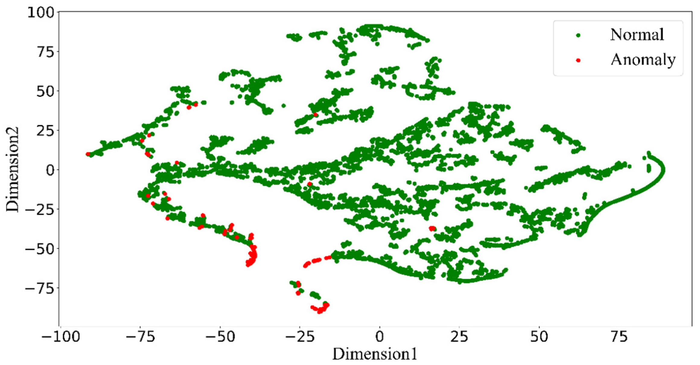
In the Life Cycle Cost–t-SNE–DBSCAN–Elman–Fisher model, the density-based spatial clustering of applications with noise was first used to screen outliers in the cost data set of the equipment, and it was found that outliers accounted for about 1.92%. In order to avoid the existence of outliers affecting the accuracy of subsequent calculations, the outliers in the data were marked as the vacancy value. There were vacancy values in the data set after processing. In order to ensure the rationality of the data, the random forest interpolation method was used to fill the vacancy values, and a complete and reasonable data set was obtained. The degree of dispersion of the data set after filling was obviously improved. Due to the randomness of equipment failure, the Elman neural network was used for random simulation to calculate the average annual entire life-cycle cost of equipment. Finally, Fisher-ordered segmentation was used to calculate the retirement life interval of equipment. In this paper, the density-based spatial clustering of applications with a noise model was used to calculate that the decommissioning interval of a 35 kV voltage transformer of an enterprise is 31 to 41 years. The results can provide references for the equipment decommissioning of enterprises. In other words, the safety and economy of the equipment are considered, which is conducive to the optimization of the technical renovation and overhaul strategy of the equipment. The safe and stable operation of equipment is the basis for the development of energy enterprises. In actual life, most enterprises pay too much attention to the stable operation of equipment and ignore the income generated by the equipment itself. When the equipment fails, they blindly carry out maintenance to keep it working, but this approach can easily cause a waste of funds. When the equipment runs for a certain number of years, its operation and maintenance costs will be greater than the income generated by the equipment itself. At this time, if the equipment can be maintained, it is not conducive to the sustainable development of the enterprise. In practical application, the model presented in this paper can be used to predict the interval of the equipment’s retirement life, and the optimal retirement life can be obtained by combining expert opinions. When the optimal retirement life is reached, the equipment retirement will be conducive to the optimization of the strategy of technical renovation and overhaul of enterprises and the development of enterprises.

Although this model is innovative in relation to the traditional process of finding the entire life-cycle cost and decommissioning life, there are still directions that need to be worked on in the future, for example, the Elman neural network model cannot perfectly represent the real situation of the equipment due to the limitations of the data and the model itself; the interpolation of vacancy values needs to be more scientific and reasonable; the selection of cost types needs to be optimized, and further research should be conducted in the future with the help of equipment costs. Further research should be carried out to find out which costs of the equipment are used to calculate the entire life-cycle cost and decommissioning life more reasonably and accurately; the density-based spatial clustering of applications with noise model should be used to calculate the entire life-cycle cost and decommissioning life of other electrical equipment; to explore these in depth, further research will be carried out in the future.

5. Innovation and Contribution

The safety and stability of energy equipment are the basis for the normal operation of enterprises and the well-being of people, but for the long-term development of enterprises, not only should the safety of the equipment be considered, but the efficiency of the output of the equipment should also be taken into account. When the equipment is past its retirement life, maintenance can lead to costs that are greater than the benefits, resulting in a waste of funds, affecting the long-term development of the enterprise. In order to improve the traditional operation and maintenance model, this paper proposes the LC–TD–EF model to calculate the decommissioning life of the equipment, after reaching the service life, which can effectively reduce the waste of money and energy consumption.

The LC–TD–EF model proposed in this paper improves the traditional method of calculating LCC and decommissioning life to make the calculated equipment decommissioning life more scientific and reasonable. This paper presents the following innovations: (1) Before the LCC cost calculation first used DBSCAN to screen the data set for outliers, the screened outliers were marked as the vacancy, and then, random forest was used to fill in the vacant values. The complete data set was obtained. This pre-processing of the data eliminated errors due to inadvertent recording or misclassification and made the data set more reasonable and accurate; (2) The Elman Neural Network was used to simulate the costs stochastically, instead of the traditional averaging process, taking into account the “haphazardness” and “minor probability” of device failures, making calculated LCC costs more scientific; (3) The use of Fisher’s ordered partitioning to calculate the equipment’s retirement life interval is more reasonable and convincing than the traditional economic life, and the company can choose the equipment’s retirement time in the interval according to the actual operation situation, and has the autonomy.

This paper has the following contributions: (1) The traditional model for calculating LCC and decommissioning life is improved by using the LC–TD–EF model to find the decommissioning life interval of the equipment, which takes into account the outliers and vacancies of the cost and the “haphazardness” and “minor probability” of devices failure. This makes the calculated economic life more accurate; (2) The model calculates the equipment decommissioning life interval, below the decommissioning life, the value of the equipment is not fully developed, above the decommissioning life, the cost invested in the equipment will be greater than the benefits of the equipment itself, resulting in a waste of funds, so the use of the life in the decommissioning life interval is a reference for the optimal decommissioning life of equipment, to optimize the management strategy of the enterprise’s technological reform and overhaul, which is conducive to the long-term development of enterprises. This is beneficial to the long-term development of the enterprise.

For future optimization, the following aspects can be considered. To estimate the LCC, a large amount of accurate historical cost data is required, and it is inevitable that it will take a lot of time, manpower, and material resources to collect historical data and find the cost estimation equation separately for each LCC estimation. The operating environment in which power equipment is located is complex and there are many factors influencing failure. The traditional strategy for companies is to use the design life of the equipment (the manufacturer’s specified equipment retirement life) as the retirement life. It is a difficult challenge to convince companies to accept the retirement life calculated by the LC–TD–EF model, and for some small energy companies with less capital and smaller equipment, the retirement life is no longer fully applicable, and the optimization of the technical overhaul strategy for small companies may be further optimized. The optimization of technical overhaul strategies for small enterprises may be further optimized.