Feature Selection and Damage Identification for Urban Railway Track Using Bayesian Globally Sparse Principal Component Analysis

Abstract

Urban railway track infrastructures often suffer from damage that affects their service performance due to a variety of factors. In this study, an unsupervised feature selection and damage identification method based on globally sparse probabilistic principal component analysis (PCA) is proposed for urban railway tracks using the monitoring data of train-induced dynamic responses. A Bayesian framework is proposed for generating principal components on a basis of vectors (original variables) with a global sparseness pattern instead of separate patterns in a traditional sparse PCA. In this framework, a variational expectation-maximization algorithm is employed to obtain the tractable calculation of the marginal likelihood function for learning all uncertain parameters of the Bayesian model. The obtained principal components are linear combinations of the very same set of important variables, making our method better interpretable than the traditional sparse PCA. We can clearly understand which original variables are most relevant for describing the data. The track damage is identified simply by discriminating the corresponding measured dynamic responses using the binary elements of the latent vector inferred from the Bayesian globally sparse PCA algorithm. The usefulness is demonstrated by successfully identifying the track bed plate crack damage through the actual train-induced dynamic responses collected from the structural health monitoring system of an urban railway track infrastructure, where the method is able to achieve $F_1$ scores of 90% or higher for various scenarios.

1. Introduction

With the development of urbanization in recent years, urban railway tracks have been widely constructed and have become important transportation infrastructure. The track directly bears the train load, and its geometric shape and position are easily affected by the deformation of the foundation, so the track is the work focus of daily maintenance. Under the coupling effect of various factors such as vehicle load, environmental erosion and material aging, the existing track structure performance gradually degrades, resulting in a variety of damages, which usually occur at the rail, fasteners and roadbed. When the damage accumulates to a certain degree, it will seriously threaten the safety of urban railway tracks. Therefore, timely and reliable identification of possible damage to urban railway tracks is an urgent issue that is of great significance for the maintenance and operation of urban railways as well as for ensuring traffic safety [1].

The current track inspection methods mainly include daily manual inspection, static track inspection and dynamic inspection. The most typical one is manual inspection [2], which determines whether damage occurs by visual observation and simple instrumentation measurement. However, there are several problems with manual inspection. First of all, daily manual inspection can only be carried out during daylight hours and cannot be conducted during the normal operation of the track, so the damage cannot be found in time. In addition, a large number of workers are needed for daily inspection to ensure the effectiveness of the inspection. Recently, with the development of artificial intelligence, some machine vision-based inspection algorithms have been developed for efficient automatic surface damage detection [3]. However, it is difficult for hidden or inconspicuous damage to be identified using these techniques.

Structural health monitoring can well solve the above bottlenecks by installing sensors on tracks to sense, collect, transmit and process monitoring data in real time and has become an important way to ensure the safety of urban rail transit and other transportation infrastructure in service. Based on the monitoring data, a wide variety of damage detection methods have been proposed in recent years, including model-based and data-driven methods. In the past, model-based approaches [4,5], which required an accurate structural model to identify possible damage, were the main trend. To ensure the accuracy of the structural model, a large amount of high-quality measured data is required for model calibration and updating. The susceptibility to inevitable modeling errors and the requirement of costly resources have also limited the success of these models. With the advancement of pattern recognition and machine learning in the last decade, data-driven methods [6,7,8] provide a promising computational tool to avoid the issues mentioned above without models. These methods extract some damage-sensitive signal features and recognize (or identify) the damage by the measurement of data abnormalities, that is, changes in the exacted feature pattern. The different types of track damage identification methods and their drawbacks are summarized in

Table 1. Summary of track damage identification methods.

Methods	Identification Means	Drawbacks
Manual inspection [2]	Visual observation and simple instrumentation measurement	Inability to detect damage in time, difficulty in detection of inconspicuous damage
Model-based method [4,5]	Constructing an accurate structural model	Requires large amounts of high-quality data for model calibration and updating
Data-driven method [6,7,8]	Extract damage-sensitive signal features	No physical information about the structure is incorporated

.

Principal component analysis (PCA) [9,10], a well-established technique for feature extraction and dimensionality reduction, has numerous applications in statistical learning, such as handwritten numeral recognition [11,12], face recognition [13,14] and feature analysis [15,16]. This technique is especially effective for dimensionality reduction in big data. For example, Gadekallu et al. [17] applied PCA to tomato disease classification to effectively reduce the relevant features in the dataset, further reducing the training time of the machine learning algorithm. Reddy et al. [18] analyzed and compared dimensionality reduction techniques on big data and found that PCA is superior to linear discriminant analysis. The conventional PCA approaches seek linear projections of the original variables onto a “principal” subspace with the directions of maximum variance by means of eigenvalue decomposition. However, the feature extraction procedure in conventional PCA is not simple to interpret, as the principal components are linear combinations of all single original variables for multivariate data. To tackle such problems, sparse PCA was developed by involving an automatic selection of the appropriate model dimensionality with high-dimensional data; i.e., the principal components obtained by sparse PCA are linear combinations of only a few important variables, which facilitates the interpretation of data feature selection in practice. The main methods commonly used are the addition of a regularization term [19,20] and the use of promoting sparsity of a prior distribution for the coefficients of the projection matrix [21,22]. However, the sparseness patterns of the original variables for each principal component may be different, and thus we need to understand which original variables are active for interpreting each principal component separately. In this study, the monitoring dynamic responses of the track bed plate in each measurement area during the pass of each train are truncated and employed for analysis. Due to the unified structural layout of the track and trains as well as the similar mechanism of the train loads, it is expected that the monitoring vibration data of the track induced by each train should share some common features. These common features need to be robustly mined using an effective PCA method. To this end, a Bayesian globally sparse PCA method [23] is first introduced for urban railway track damage identification in this study, with the aim of globally selecting which original variables are relevant for describing the data. Rather than observing the principal components, the global sparseness pattern of the selected original variables recognized by Bayesian globally sparse PCA is employed as a damage-sensitive indicator. This is because, in a damage identification problem, the damage-induced feature change may not be a global characteristic of the data matrix (may include both the undamaged and damaged signals) and cannot be selected by Bayesian globally sparse PCA considering the infrequent occurrence of the track damage. The method is applied to the actual monitoring data of a subway line, and a comparative study with the state-of-the-art Bayesian sparse PCA method is also performed for demonstrating the superiority of the presented method. The method is effective in identifying potential track damage in time by monitoring data abnormalities, even if the track is in service or the damage is inconspicuous. This is also the main contribution of the paper.

The rest of this paper is organized as follows: A Bayesian globally sparse PCA method for unsupervised feature selection and subway track damage identification is introduced in Section 2. Illustrative examples are presented in Section 3 to validate the proposed method, and the conclusions drawn are presented in Section 4.

2. Bayesian Globally Sparse PCA for Feature Selection and Damage Identification

2.1. Bayesian PCA Model

In this study, the monitoring dynamic response data of the track bed plate in each measurement area during the pass of each train will be truncated and employed for analysis. Each D-dimensional measurement data (column vector) is denoted as $x_n$, and then we have a data matrix $X={\left[x_1,\dots ,x_N\right]}^T\in {ℝ}^{N\times D}$. PCA tries to find a linear projection of the data onto a principal subspace of much lower dimensionality, under which the variance is preserved as much as possible.

Due to the benefits of probabilistic modeling, a probabilistic formulation of PCA [24] was well established, which forms the basis for diverse Bayesian formulations [25,26,27]. The formulation starts from the introduction of an explicit latent vector $z\in {ℝ}^M$ corresponding to the principal-component subspace. A zero-mean and unit-covariance Gaussian prior probability density function (PDF) is assumed for the latent vector $z$:

$$p\left(z\right)=\mathcal{N}(z|\mathbf{0},I_M)$$

(1)

A Gaussian likelihood function of $z$ can also be defined as follows:

$$p\left(x|P,z,{\sigma }^2\right)=\mathcal{N}(x|Pz,{\sigma }^2{I}_D)$$

(2)

Probabilistic PCA assumes that the observed variable $x$ can be expressed by a linear transformation of the latent vector $z$ with a Gaussian prediction error term $\mathsf{\epsilon }$, i.e., $x=Pz+\mathsf{\epsilon }.$ Here, $P\in {ℝ}^{D\times M}$ is a loading matrix, and $\mathsf{\epsilon }~\mathcal{N}(\mathsf{\epsilon }|\mathbf{0},{\sigma }^2{I}_{\mathit{D}})$, which is the maximum entropy distribution [28,29].

It can be seen that the likelihood function of $P$ and ${\sigma }^2$ can be obtained effectively by integrating out the latent vector $z$:

$$\begin{gathered} p\left(x|P,{\sigma }^2\right)={\displaystyle \int }p\left(x|P,z,{\sigma }^2\right)p\left(z\right)dz \\ ={\displaystyle \int }\mathcal{N}(x|Pz,{\sigma }^2{I}_D)\mathcal{N}(z|\mathbf{0},I_M)dz=\mathcal{N}(x|\mathbf{0},P{P}^T+{\sigma }^2{I}_D) \end{gathered}$$

(3)

An automatic relevance determination prior [30] used to be defined for loading matrix $P$ in the Bayesian formulation of PCA [25] for determining the effective dimensionality of the latent vector $z$ automatically. In addition, a non-informative prior can be assigned for the prediction error variance ${\sigma }^2$. Then the uncertain parameters $P$ and ${\sigma }^2$can be learned from their posterior PDF $p\left(P,{\sigma }^2|x\right)$, which is computed from Bayes’ Theorem:

$$p\left(P,{\sigma }^2|x\right)\propto p\left(x|P,{\sigma }^2\right)p\left(P\right)p\left({\sigma }^2\right)$$

(4)

which is proportional to the product of the likelihood function and prior PDF.

For conventional sparse PCA [21,22], its loading matrix $P$ would be expected to have few nonzero coefficients. However, each principal component usually selects different relevant variables (data columns) in data matrix $X$ because we do not have the same sparseness pattern, i.e., they cannot be expressed as the linear combination of the same active variables in $X$. This will lead to the consequence that we must interpret each principal component separately, which may be inconsistent with the analysis of the track monitoring data. Due to the unified structural layout of the track and the similar mechanism of the train loads, it is expected that the monitoring vibration data of the track induced by each train should share some common features. Meanwhile, considering the infrequent occurrence of the track damage, the damage-indued feature may not be a global characteristic of the data matrix $X$ (may include both the undamaged and damaged signals) and cannot be selected by Bayesian globally sparse PCA. Therefore, the same sparseness pattern of all principal components called global sparseness [23] is adopted in this study, and we can use these global characteristics as a damage-sensitive indicator.

In the next subsection, a Bayesian inference framework for globally selecting relevant features is formulated. Note that the other motivation is that we can obtain orthogonal and uncorrelated principal components when performing PCA on the relevant variables with global sparseness [23].

2.2. Bayesian Inference for Globally Sparse PCA

For the purpose of enforcing the global sparseness, all elements in several rows of the loading matrix $P$ should be constrained to be zero [23]. To realize this, a binary vector $o\in {\left\{0,1\right\}}^D$ whose nonzero entries correspond to those relevant variables in $x$ is introduced. This leads to the following linear model:

$$x=OPz+\mathsf{\epsilon }$$

(5)

where $O=\mathrm{diag}\left(o\right)$. Note that the feature selection (selecting the active variables, which are the elements in vector x or the columns of the data matrix $X$) can be realized by simply observing the binary vector $o$, and thus the loading matrix $P$ can be regarded as latent parameters in the formulation below.

Assume that the coefficients in the loading matrix $P$ are independently and identically distributed. The prior for loading matrix $P$ is assigned as an isotropic Gaussian distribution:

$$p\left(P|\alpha \right)={{\displaystyle \prod }}_{d=1}^D{{\displaystyle \prod }}_{m=1}^M\mathcal{N}(P_{dm}|0,{\alpha }^{-1})$$

(6)

Similar to Equation (3), the likelihood function for the loading matrix $P$ given observations $x$ is obtained as follows:

$$\begin{gathered} p\left(x|o,P,{\mathsf{\sigma }}^2\right)={\displaystyle \int }p\left(x|o,P,z,{\mathsf{\sigma }}^2\right)p\left(z\right)\mathrm{d}z \\ ={\displaystyle \int }\mathcal{N}(x|OPz,{\mathsf{\sigma }}^2{I}_{\mathrm{D}})\mathcal{N}(z|\mathbf{0},I_{\mathrm{M}})\mathrm{d}z=\mathcal{N}(x|\mathbf{0},OP{P}^{\mathrm{T}}{O}^{\mathrm{T}}+{\mathsf{\sigma }}^2{I}_{\mathrm{D}}) \end{gathered}$$

(7)

Based on the Bayesian modeling above, the acyclic graph of the hierarchical Bayesian model for Bayesian globally sparse PCA is shown in Figure 1, where each arrow denotes the conditional dependencies used in the model.

From the evidence-maximizing procedure in Bayesian learning [31,32,33], it is known that the uncertain parameters $\left\{o,\mathsf{\alpha },{\sigma }^2\right\}$ can be learned by maximizing the following marginal likelihood function (evidence function) if non-informative priors are assigned for $\left\{o,\mathsf{\alpha },{\sigma }^2\right\}$:

$$p\left(x|o,\mathsf{\alpha },{\mathsf{\sigma }}^2\right)={\displaystyle \int }p\left(x|P,o,{\mathsf{\sigma }}^2\right)p(P|\mathsf{\alpha })\mathrm{d}P$$

(8)

However, this integral of the matrix above seems intractable and hard to be computed analytically. Furthermore, it is a challenging task to determine the value of binary vector o, as there is a total of $2^D$ possible values for o because of its discreteness. It is still difficult even if the marginal likelihood has a closed-form expression. Therefore, a simple continuous relaxation of the problem is considered by replacing o with a continuous vector $v\in {\left[0,1\right]}^D$. Then the linear model for the observations becomes

$$x=VPz+\mathsf{\epsilon }$$

(9)

where $V=\mathrm{diag}\left(v\right)$. For a more concise representation, the uncertain parameter vector to be learned is denoted as $\mathsf{\theta }=\left\{v,\alpha ,{\sigma }^2\right\}$. Both the reduced dimensional data $z_i$ and the matrix $P$ are considered as latent variables. Next, we use the variational approach [34] to maximize the evidence function $p\left(X|\mathsf{\theta }\right)$:

$$p\left(X|\mathsf{\theta }\right)={\displaystyle \sum }_Z{\displaystyle \sum }_{P}p\left(X,Z,P|\mathsf{\theta }\right)$$

(10)

Given a variational distribution q over the space of latent variables, its logarithmic form can be decomposed as follows:

$$\ln p\left(X|\mathsf{\theta }\right)=ℒ\left(q,\mathsf{\theta }\right)+\mathrm{KL}\left(q||p\right)$$

(11)

$$\begin{gathered} ℒ\left(q,\mathsf{\theta }\right)={\displaystyle \sum }_Z{\displaystyle \sum }_{P}q\left(Z,P\right)\ln p\left(X,Z,P|\mathsf{\theta }\right)-{\displaystyle \sum }_Z{\displaystyle \sum }_{P}q\left(Z,P\right)\ln q\left(Z,P\right) \\ ={\mathrm{E}}_q\left[\ln p\left(X,Z,P|\mathsf{\theta }\right)\right]+\mathrm{H}\left[q\left(Z,P\right)\right] \end{gathered}$$

(12)

$$\mathrm{KL}\left(q||p\right)=-{\displaystyle \sum }_Z{\displaystyle \sum }_{P}q\left(Z,P\right)\ln \left\{\frac{p(Z,P|X,\mathsf{\theta })}{q\left(Z,P\right)}\right\}$$

(13)

where $Z={\left[z_1,\dots ,z_N\right]}^T\in {ℝ}^{N\times M},$ $ℒ\left(q,\mathsf{\theta }\right)$ is a generic function of the variational probability distribution q, $\mathrm{KL}(q||p)$ represents the KL divergence between the variational distribution q and the true distribution $p$, and $\mathrm{H}\left[q\left(Z,P\right)\right]$ represents the entropy of the probability distribution $q\left(Z,P\right)$. Since the KL divergence $\mathrm{KL}(q||p)$ is non-negative, $ℒ\left(q,\mathsf{\theta }\right)$ becomes a lower bound on the log-evidence function $ℒ\left(q,\mathsf{\theta }\right)\le \ln p\left(X|\mathsf{\theta }\right)$. The problem now translates into maximizing the $ℒ\left(q,\mathsf{\theta }\right)$. Based on the mean-field theory [35], the distribution of the latent variables is approximated as follows:

$$q\left(Z,P\right)=q\left(Z\right)q\left(P\right)$$

(14)

We can find the maximum likelihood estimations of the uncertain parameters using the expectation maximization (EM) algorithm [34]. For the E-step, $ℒ\left(q,\mathsf{\theta }\right)$ is maximized with respect to q, while the parameter $\mathsf{\theta }$ remains fixed. The variational posterior distribution of the latent variables which maximizes the $ℒ\left(q,\mathsf{\theta }\right)$ is given by

$$q\left(Z\right)={\displaystyle \sum }_{\mathrm{i}=1}^{\mathrm{N}}\mathcal{N}(z_{\mathrm{i}}|{\mu }_{\mathrm{i}},\Sigma )$$

(15)

$$q\left(P\right)={\displaystyle \sum }_{\mathrm{k}=1}^{\mathrm{D}}\mathcal{N}({\mathrm{p}}_{\mathrm{k}}|m_{\mathrm{k}},S_{\mathrm{k}})$$

(16)

where, for all $i\in \left\{1,\dots ,N\right\}$ and $k\in \left\{1,\dots ,D\right\}$

$${\mathsf{\mu }}_{\mathrm{i}}=\frac{1}{{\sigma }^2}\Sigma M^{\mathrm{T}}V{x}_i$$

(17a)

$$m_{\mathrm{k}}=\frac{{\mu }_k}{{\sigma }^2}{S}_{\mathrm{k}}{\displaystyle \sum }_{i=1}^N{\mathrm{x}}_{\mathrm{i},\mathrm{k}}{\mathsf{\mu }}_{\mathrm{i}}$$

(17b)

$${\Sigma }^{-1}=I_{\mathrm{M}}+\frac{1}{{\sigma }^2}{M}^{\mathrm{T}}{V}^{\mathrm{T}}M+\frac{1}{{\sigma }^2}{\displaystyle \sum }_{k=1}^D{\mu }_k^2{S}_{\mathrm{k}}$$

(17c)

$$S_{\mathrm{k}}^{-1}={\alpha }^2{I}_{\mathrm{M}}+\frac{N{\mu }_k^2}{{\sigma }^2}\Sigma +\frac{{\mu }_k^2}{{\sigma }^2}{\mathit{ℳ}}^{\mathrm{T}}\mathit{ℳ}$$

(17d)

where$M={\left(m_1,\dots ,m_D\right)}^T$ and $\mathit{ℳ}={\left({\mathsf{\mu }}_{\mathbf{1}},\dots ,{\mathsf{\mu }}_N\right)}^T$.

In the next M-step, keeping q unchanged, $ℒ\left(q,\mathsf{\theta }\right)$ is maximized with respect to the parameter $\mathsf{\theta }$ to obtain the updated value ${\mathsf{\theta }}^{new}$. The updated parameters are

$${\alpha }^{new}={\left(\frac{1}{DM}{\displaystyle \sum }_{k=1}^D\mathrm{Tr}\left(S_{\mathrm{k}}+m_{\mathrm{k}}{m}_{\mathrm{k}}^{\mathrm{T}}\right)\right)}^{-1/2}$$

(18)

$${\left({\sigma }^2\right)}^{new}=\frac{\mathrm{Tr}\left(X^{\mathrm{T}}X-2XVM\mathit{ℳ}\right)}{ND}+\frac{1}{ND}{\displaystyle \sum }_{i=1}^N{\displaystyle \sum }_{k=1}^D{\mu }_k^2\mathrm{Tr}\left[\left(\Sigma +{\mu }_{\mathrm{i}}{\mu }_{\mathrm{i}}^{\mathrm{T}}\right)\left(S_{\mathrm{k}}+m_{\mathrm{k}}{m}_{\mathrm{k}}^{\mathrm{T}}\right)\right]$$

(19)

and, for $k\in \left\{1,\dots ,D\right\}$,

$$v_k^{new}={\mathrm{argmin}}_{u\in \left[0,1\right]}\frac{v^2}{2}{\displaystyle \sum }_{i=1}^N\mathrm{Tr}\left[\left(\Sigma +{\mathsf{\mu }}_{\mathrm{i}}{\mathsf{\mu }}_{\mathrm{i}}^{\mathrm{T}}\right)\left(S_{\mathrm{k}}+m_{\mathrm{k}}{m}_{\mathrm{k}}^{\mathrm{T}}\right)\right]-v{\displaystyle \sum }_{i=1}^N{x}_{i,k}{m}_{\mathrm{k}}^{\mathrm{T}}{\mathsf{\mu }}_{\mathrm{i}}$$

(20)

In the final step, for global sparse feature selection purpose, the binary vector o$\in {\left\{0,1\right\}}^D$ should be obtained by the transformation from the most probable values of continuous vector $v$. One of the straightforward approaches is to pick a threshold $\tau$, and elements in $v$ greater than this threshold are set to 1. However, determining how to pick a suitable threshold would be an issue.

In [23], a transformation procedure has been formulated based on the formulation of an exact form of the marginal likelihood function. We define the set of vectors $o^{\left(k\right)}$ as the binary vectors such that, for each k, the k top coefficients of $v$ are set to 1 and the others are set to 0. The marginal likelihood function is evaluated for all ${\left\{o^{\left(k\right)}\right\}}_{k=1}^D$, and the number of relevant variables $k$ is chosen such that the marginal likelihood is maximized. The advantage of this is that we only need to deal with a family of D models instead of $2^D$. Even when the number of input variables is large, our method still guarantees high computational efficiency.

After obtaining the binary vector o, the original variables which are most relevant for describing all principal components are determined, so that all principal components obtained are linear combinations of these selected variables. This has better interpretability than traditional sparse PCA in which each principal component is a linear combination of different original variables.

2.3. Feature Selection and Damage Identification Procedure for Urban Railway Track

In Section 2.2, the feature selection of the track monitoring data is realized by the global sparseness pattern of the selected original variables for PCA analysis. The track damage then can be identified from the judgment of abnormalities in the nearby measurement data, if the structural local responses are measured (in the illustrative example in Section 3, the strain responses are collected by fiber optic grating array sensor). The whole procedure for feature selection and urban railway track damage identification can be summarized as follows:

(1)

Based on the inputs of the data matrix $X\in {ℝ}^{N\times D}$ of track monitoring and dimension $M$ of the latent space in $z$, the EM algorithm is performed iteratively from the initially selected values to infer the most probable values of the uncertain parameter $\left\{v,\alpha ,{\sigma }^2,{\mathsf{\mu }}_1,\dots ,{\mathsf{\mu }}_N,m_1,\dots ,m_D,S_1,\dots ,S_D, \Sigma \right\}$ using Equations (17)–(20).

(2)

The most probable values of continuous vector v are transformed into a binary vector $o\in {\left\{0,1\right\}}^D$, and the selected relevant variables (data columns) in the data matrix $X$ correspond to the nonzero entries in vector $o$.

(3)

The binary elements (0 and 1) of the inferred vector $o$ are employed to distinguish whether each monitoring data piece is associated with an abnormal (element value is 0, indicating there is damage occurring in the areas near the sensor) or normal (element value is 1, indicating there is no damage occurring in the areas near the sensor) condition.

(4)

Inspection of the track is performed in the areas near the sensor for precise localization of damage.

3. Engineering Verification

In this section, the analysis of the monitoring data collected from the SHM system of an urban railway track in China is conducted to verify the effectiveness and practicality of the proposed method. To present a further quantitative presentation, three metrics are adopted to evaluate the damage identification performance. Moreover, the influence of the dimensionality of latent variable $z$ on the damage identification performance is also investigated.

3.1. Urban Railway Track Monitoring Data

The urban railway investigated in this study has been put in service in the last few years. The line is laid seamlessly, and welded joints are employed at the track joints. The concrete track bed was cast on-site, and the short rail sleepers were embedded in it to form the integral rail bed.

A fiber optic grating array sensor system is employed for track monitoring (see Figure 2a). The fiber optic cable is arranged on the surface of the track bed plate along the track (parallel to the track) in a long section. The measurement areas are connected in series, and each measurement area has a length of 5 m along the track, which is also the distance between adjacent fiber Bragg gratings (FBGs). The structural vibrations are calculated by detecting the phase change of the optical waves by micro-vibrations between adjacent FBGs, and the measured vibration for each measurement area is the average dynamic strains between the adjacent FBGs. The sampling frequency is 1000 Hz.

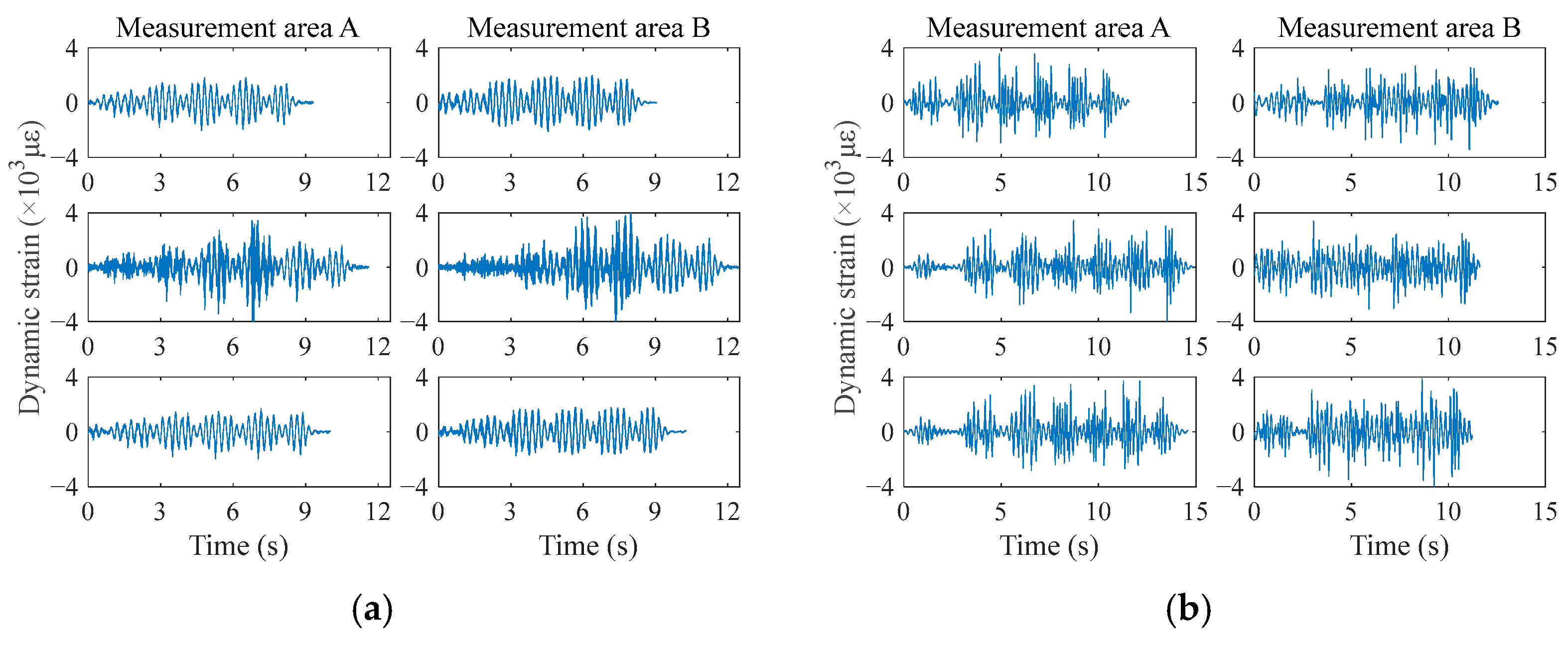
Figure 2b displays a crack occurring in the track bed plate, which may cause groundwater to penetrate into the bed. The length, depth and average width of the crack are around 1.1 m, 0.5 m and 2 mm, respectively. The track plate crack is located near the location where the two measurement areas are connected, and the two measurement areas will be denoted as measurement areas A and B (see Figure 2a). The direction of the crack is somewhat inclined at the edge of the track plate and then becomes approximately perpendicular to the track at the middle of the plate. As each train passes, the monitored train-induced dynamic responses of measurement areas A and B before and after the occurrence of damage are truncated for analysis, and the representative signals are shown in Figure 3.

It can be seen from Figure 3 that the lengths of the signals vary due to the varying speeds of trains passing through the measurement area. In order to align the monitoring data for PCA calculation, one piece of the data corresponding to the passage of a train was referred to as the standard signal, and the initial measurement times and train speeds of other time series were adjusted by translation and scaling in the time domain. Interpolation correction was then carried out for the misaligned data, and the one with the greatest correlation with the standard signal was selected as the alignment result. The signals after data alignment are demonstrated in Figure 4.

From the comparison of the signals during the periods without and with damage in Figure 4, it can be seen that there is some difference in the waveforms; i.e., some waveforms are more spurious in the time domain for damaged signals, but this is not true for all measurements. However, to avoid false and missed identifications, a reliable method is required to identify track damage in a timely manner to guarantee the safe operation of urban railway transportation. In the next subsection, the performance of the damage identification method based on Bayesian globally sparse PCA is investigated.

3.2. Urban Railway Track Damage Identification Performance

As described in Section 2, the binary elements (0 and 1) of the binary vector $o$ inferred from the Bayesian globally sparse PCA algorithm are employed to discriminate whether the monitoring data are associated with damaged (element value is 0) or undamaged (element value is 1) states. To verify the effectiveness of the proposed method, we specifically designed two scenarios. The main difference between these two is whether all data columns in the data matrix $X$ for feature selection are collected from the same measurement area or not. This is useful for practical applications if we are able to identify damage effectively using even monitoring data collected from different measurement areas for PCA analysis.

3.2.1. Scenario 1: Verification in Single Monitoring Area

In this subsection, 130 columns of data pieces, each with the number of points $N=7346$ (each corresponding to the passage of a train, i.e., $D=130$) collected from the same measurement area, are employed to compose the data matrix $X$ for PCA implementation.

Note that the original variables (data columns) for feature selection in the globally sparse PCA here have 130 dimensions, we need to globally determine the most relevant data columns for yielding the principal components of data matrix $X$. The dimension M of the latent variable z is set to be 10. We first run the Bayesian globally sparse PCA approach to analyze the track monitoring data for measurement area B. The measured data are divided into two cases of 130 columns of undamaged data, and 115 columns of undamaged data plus 15 columns of damaged data, and the first six principal components obtained in both cases are shown in Figure 5. The principal components are a small set of summary indices that can retain most of the information in the original set of data variables. The maximum possible information contained in matrix $X$ is squeezed into the first-order principal component, the maximum remaining information is squeezed into the second-order principal component, and so on. However, as can be observed from the figures, the computed principal components are not very sensitive to damage and thus are not applicable for urban railway damage identification. This also indicates that the infrequent damage cannot induce a significant change in the key directions for constructing the data matrix $X$. Next, the global sparseness pattern vector $o$ recognized by Bayesian globally sparse PCA will be investigated.

To examine the damage identification performance of the global sparse pattern vector $o$, we run the Bayesian globally sparse PCA approach using the data matrix $X$ consisting of 115 columns of undamaged data and 15 columns of damaged data from measurement areas A and B, separately. By comparing binary elements (0 and 1) of the vector $o$ with the actual ones and counting the number of correct identifications for both the undamaged and damaged classes, the confusion matrices between the actual damage data and the damage identification results can be obtained, as shown in Figure 6. The results show that for data from measurement area A, our algorithm achieves 100% identification accuracy for the damaged data columns, while for the undamaged data columns, the accuracy decreases to 80.87%; i.e., 19.13% of the undamaged data are incorrectly identified as damaged. Therefore, our method is effective in avoiding missed identifications, even though false identifications sometimes occur. The results are similar for the data from measurement area B: the accuracies are 100% and 87.83% for damaged and undamaged data, respectively.

To further quantify the performance of damage identification, three metrics, precision, accuracy and $F_1$ score, are introduced [36]; they are defined as follows:

$$Precision=\frac{t_p}{t_p+f_p}$$

(21)

$$Accuracy=\frac{t_p+t_n}{t_p+t_n+f_p+f_n}$$

(22)

$$F_1=\frac{2}{\frac{1}{Precision}+\frac{1}{Recall}}=2·\frac{Precision·Recall}{Precision+Recall}\times 100\%$$

(23)

where $Recall=\frac{t_p}{t_p+f_n}$; $t_p,$ $f_p$, $f_n$, and $t_n$ refer to true positive, false positive, false negative and true negative, respectively. Regarding the three indices, precision indicates the proportion of the data which are correctly discriminated as the undamaged class, accuracy indicates the proportion of the data which are correctly discriminated as their associated classes (undamaged or damaged) and $F_1$ score is an index that comprehensively takes precision and recall into consideration. The values of the three metrics corresponding to the results in Figure 6 are shown in

Table 2. Specific values of damage identification performance metrics for Scenario 1.

Metrics (%)	Measurement Area A	Measurement Area B
Precision	100.00	100.00
Accuracy	83.07	89.23
$F_1$	89.42	93.51

. For a more intuitive comparison, we also present the results as a histogram in Figure 7.

Figure 7 and Table 2 show that among the three indices, the accuracy index has the lowest value ($83.07\%$). This means that our algorithm is able to accurately identify the damage status for more than $83\%$ of the monitoring data. The index with the highest values is precision, which can even reach $100\%$, indicating that there is no missed identification occurring for our method, which is essential for reliably finding track damage. $F_1$ scores, as a comprehensive measure of performance, possess the values of $89.42\%$ and $95.31\%$ for the data from the two measurement areas, respectively. These are reasonably high since the monitoring track dynamic responses induced by each train should be similar to each other, and so share some global spareness which can be extracted by the presented globally sparse PCA. Meanwhile, the feature change caused by the damage may not be a global characteristic of the data matrix $X$. Therefore, the damaged data can be discriminated from others with high accuracy.

For further investigation of the damage identification performance purpose, we also investigate the results of the state-of-the-art Bayesian sparse PCA presented in [21], in which the prior of the loading matrix is modeled as a spike-and-slab prior, to analyze the monitoring data for the track structure. Global sparseness can also be achieved by restricting the sparse mode to joint row sparsity. The confusion matrices between the actual damage data and the damage identification results are shown in Figure 8. It can be observed that almost all data columns are identified as undamaged; thus, this method is not effective in identifying damage, although global sparsity is also imposed in this method.

In Figure 9, we also examine the sensitivity of the proposed method to the latent variable dimension $M$. Three other values, namely $15$, $20$ and $25$, are chosen to calculate the three indices in Equations (21)–(23). There are only slight variations for all three indices, indicating that our method is robust to the latent variable dimensions. This is presumably because the latent variable dimensions only determine the number of principal components, which has no significant influence on the globally selected variables, and so the damage identification results.

3.2.2. Scenario 2: Verification across Monitoring Areas

In this subsection, we also investigate the scenario in which data columns in the data matrix $X$ are collected from both measurement areas. The same size of data matrix $X$ (the number of data columns is $D=130$) as that in Scenario 1 is selected. We use “A-B” to indicate the data combination in matrix $X$ in which $100$ of the columns of undamaged data are collected from measurement area A, and $15$ columns of undamaged and $15$ columns of damaged data are collected from measurement area B; “B-A” represents the data combination in which $100$ columns of undamaged data are collected from monitoring area B, and $15$ columns of undamaged and $15$ columns of damaged data are collected from monitoring area A. The algorithm parameter settings remain the same as those in Scenario 1.

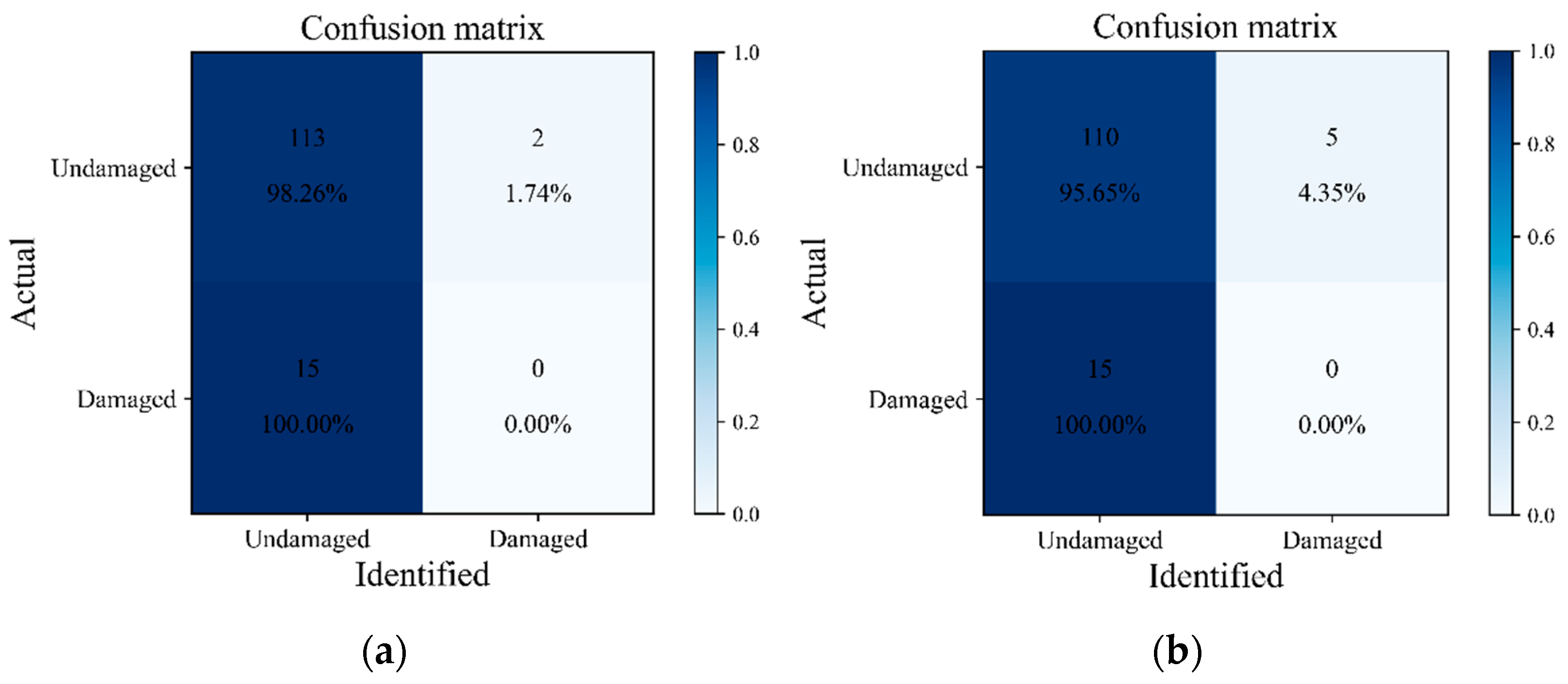
As in Figure 6, the confusion matrices between the actual and identified damage results are presented in Figure 10. The results demonstrate that for the undamaged data from different measurement areas, our algorithm is still able to identify their associated status with very high accuracy (over 90%). For the damaged data, it is also effective: 100% of the data in the first data combination are successfully identified, although for the second data combination, we only discriminate 60% of the damaged data correctly.

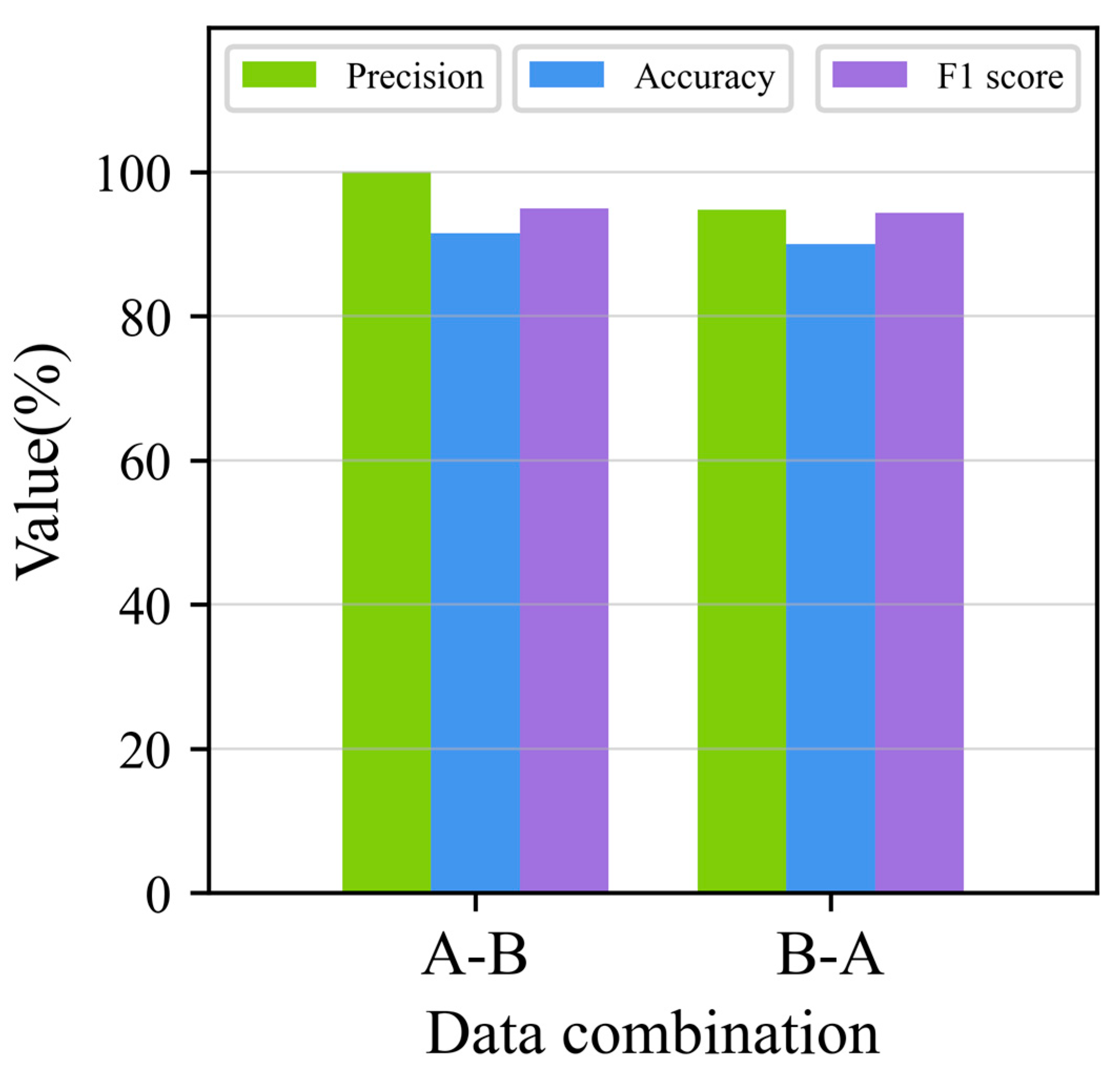
The results of the three metrics in Equations (21)–(23) for Scenario 2 are demonstrated in Figure 11 and

Table 3. Specific values of damage identification performance metrics for Scenario 2.

Metrics (%)	Measurement Area A	Measurement Area B
Precision	100.00	94.74
Accuracy	91.54	90.00
$F_1$	94.98	94.32

. Similar to the results in Figure 7 and Table 2, the lowest and highest values are found for the accuracy and precision indices, which are 90% and 100%, respectively. Moreover, $F_1$ scores of 94.98% and 94.32% can be obtained for the two data combinations, respectively. These results imply that our method still produces excellent damage identification performance even when using data from different measurement areas for PCA analysis.

Similar to Scenario 1, we also present the confusion matrices between the actual damage results and damage results identified by running Bayesian sparse PCA from [21] in Figure 12. Similar to the results in Figure 8, very few damaged data columns (6.67% and 13.33%) can be correctly identified, and this method cannot be applied for track damage identification.

It is worth noting that different crack locations and forms will result in different variations in the monitoring data features. However, in our study, track damage is identified by the judgment of abnormalities in the measurement data. On this basis, even with different crack locations and forms, we can still determine the occurrence of the track damage in the areas close to the sensor with data abnormalities.

4. Conclusions

Feature selection and extraction are essential for data-driven detection of damage to civil infrastructure. In this paper, a Bayesian approach for globally sparse probabilistic principal component analysis (PCA) is presented for unsupervised feature selection and damage identification using urban railway track monitoring dynamic response data. This is motivated by the fact that the monitoring data of train-induced dynamic responses may lie close to a principal-component subspace spanned by variables with a shared sparseness pattern and the global sparseness pattern is a damage-sensitive indicator since the damage-caused feature may be local. Different from the conventional sparse PCA methods that only find the local sparseness structures of variables for explaining the single principal components, our method aims at globally selecting the relevant features for all principal components; that is, the same active features for all principal components can be extracted automatically in an unsupervised manner. A variational expectation-maximization algorithm is employed to obtain the analytical solution of the most probable uncertain parameters by maximizing the marginal likelihood function.

The superior performance of the presented Bayesian globally sparse PCA method over the state-of-the-art Bayesian sparse PCA method is verified by the actual train-induced vibration data collected from the structural health monitoring system of an urban railway track infrastructure. Our method can handle the unsupervised feature selection problem of high-dimensional SHM data, and the track bed plate crack damage has been successfully identified by the inferred global sparse pattern. Three indexes are also presented to quantify the performance of damage identification results. With the high accuracy of actual damage identification performance, we believe that a promising method has been developed toward practical damage identification for urban railway tracks. Timely and reliable identification of possible damage to urban railway tracks based on structural health monitoring data is an urgent issue. When the damage accumulates to a certain degree, it will seriously threaten the safety of urban railway tracks. Even if the damage is not very serious, it may cause severe vibrations in the wheels and the rails during train operation, affecting the comfort of subway passengers.

In future studies, it would be useful to establish a physics-informed supervised deep learning method for track damage localization and classification, to address the limitations of the proposed approach, including the absence of the physical model information of the track plate and the incapability of estimating the damage severities and classifying the damage types. Moreover, the application of other types of tracks, including highspeed railway tracks, may also be a future direction.

References

1. Thomas, B.; DeRobertis, M. The safety of urban cycle tracks: A review of the literature. Accid. Anal. Prev. 2013, 52, 219–227. [Google Scholar] [CrossRef] [PubMed]
2. FRA (Federal Railroad Administration). Track Inspector Rail Defect Reference Manual. 2015. Available online: https://railroads.dot.gov/elibrary/track-inspector-rail-defect-reference-manual (accessed on 25 January 2023).
3. Karakose, M.; Yaman, O.; Baygin, M.; Akin, E. A new computer vision based method for rail track detection and fault diagnosis in railways. Int. J. Mech. Eng. Robot. Res. 2017, 6, 22-17. [Google Scholar] [CrossRef]
4. Xiang, C.; Li, Z.; Qi, X.; Cao, S.; Liu, H. Research on track damage identification based on the response of vehicle-rail contact point. Transp. Eng. 2022, 10, 100149. [Google Scholar] [CrossRef]
5. Alves, V.N.; de Oliveira, M.M.; Ribeiro, D.; Calcada, R.; Cury, A. Model-based damage identification of railway bridges using genetic algorithms. Eng. Fail. Anal. 2020, 118, 104845. [Google Scholar] [CrossRef]
6. Xie, J.; Huang, J.; Zeng, C.; Jiang, S.; Podlich, N. Systematic literature review on data-driven models for predictive maintenance of railway track: Implications in geotechnical engineering. Geosciences 2020, 10, 425. [Google Scholar] [CrossRef]
7. Wang, S.; Gao, J.; Lin, C.; Li, H.; Huang, Y. Condition assessment of high-speed railway track structure based on sparse Bayesian extreme learning machine and Bayesian hypothesis testing. Int. J. Rail Transp. 2022, 1–25. [Google Scholar] [CrossRef]
8. Li, S.; Wei, S.; Bao, Y.; Li, H. Condition assessment of cables by pattern recognition of vehicle-induced cable tension ratio, Eng. Struct. 2018, 155, 1–15. [Google Scholar]
9. Wold, S.; Esbensen, K.; Geladi, P. Principal component analysis. Chemom. Intell. Lab. Syst. 1987, 2, 37–52. [Google Scholar] [CrossRef]
10. Chan, T.H.; Jia, K.; Gao, S.; Lu, J. PCANet: A simple deep learning baseline for image classification? IEEE Trans. Image Process. 2015, 24, 5017–5032. [Google Scholar] [CrossRef] [Green Version]
11. W, J.; H, Y.; Z, G.; W, C. Offline handwritten numeral recognition based on principal component analysis. In Proceedings of the 2007 8th International Conference on Electronic Measurement and Instruments, Xian, China, 16–18 August 2007. [Google Scholar]
12. Almotiri, J.; Elleithy, K.; Elleithy, A. Comparison of autoencoder and Principal Component Analysis followed by neural network for e-learning using handwritten recognition. In Proceedings of the 2017 IEEE Long Island Systems, Applications and Technology Conference (LISAT), Farmingdale, NY, USA, 5 May 2017. [Google Scholar]
13. Bahurupi, S.P.; Chaudhari, D.S. Principal component analysis for face recognition. Int. J. Eng. Adv. Technol. 2012, 1, 91–94. [Google Scholar]
14. Abdullah, N.A.; Saidi, M.J.; Rahman, N.H.A.; Wen, C.C.; Hamid, I.R.A. Face recognition for criminal identification: An implementation of principal component analysis for face recognition. In AIP Conference Proceedings; AIP Publishing LLC.: Melville, NY, USA, 2017; Volume 1891, p. 020002. [Google Scholar]
15. Lu, Y.; Cohen, I.; Zhou, X.S.; Tian, Q. Feature selection using principal feature analysis. In Proceedings of the 15th ACM international conference on Multimedia, New York, NY, USA, 25–29 September 2007; pp. 301–304. [Google Scholar]
16. Ren, Y.; Koops, H.V.; Bountouridis, D.; Volk, A.; Swierstra, W.S.; Veltkamp, R.C.; Holzapfel, A.; Pikrakis, A. Feature analysis of repeated patterns in dutch folk songs using principal component analysis. In Proceedings of the 8th International Workshop on Folk Music Analysis (FMA2018), Aristotle University of Thessaloniki, Thessaloniki, Greece, 26–29 June 2018; pp. 86–88. [Google Scholar]
17. Gadekallu, T.R.; Rajput, D.S.; Reddy, M.P.K.; Lakshmanna, K.; Bhattacharya, S.; Singh, S.; Alazab, M. A novel PCA–whale optimization-based deep neural network model for classification of tomato plant diseases using GPU. J. Real-Time Image Process. 2021, 18, 1383–1396. [Google Scholar] [CrossRef]
18. Reddy, G.T.; Reddy, M.P.K.; Lakshmanna, K.; Kaluri, R.; Rajput, D.S.; Srivastava, G.; Baker, T. Analysis of dimensionality reduction techniques on big data. Ieee Access 2020, 8, 54776–54788. [Google Scholar] [CrossRef]
19. Zou, H.; Hastie, T.; Tibshirani, R. Sparse principal component analysis. J. Comput. Graph. Stat. 2006, 15, 265–286. [Google Scholar] [CrossRef] [Green Version]
20. Zou, H.; Xue, L. A selective overview of sparse principal component analysis. Proc. IEEE 2018, 106, 1311–1320. [Google Scholar] [CrossRef]
21. Ning, B. Spike and slab Bayesian sparse principal component analysis. arXiv 2021, arXiv:2102.00305. [Google Scholar]
22. Zeng, J.; Liu, K.; Huang, W.; Liang, J. Sparse probabilistic principal component analysis model for plant-wide process monitoring. Korean J. Chem. Eng. 2017, 34, 2135–2146. [Google Scholar] [CrossRef]
23. Bouveyron, C.; Latouche, P.; Mattei, P.A. Bayesian variable selection for globally sparse probabilistic PCA. Electron. J. Stat. 2018, 12, 3036–3070. [Google Scholar] [CrossRef]
24. Tipping, M.E.; Bishop, C.M. Probabilistic principal component analysis. J. R. Stat. Soc. Ser. B (Stat. Methodol.) 1999, 61, 611–622. [Google Scholar] [CrossRef] [Green Version]
25. Christopher, M.B. Bayesian PCA. In Proceedings of the 1998 Conference on Advances in Neural Information Processing Systems II, July 1999; pp. 382–388. [Google Scholar]
26. Bouveyron, C.; Latouche, P.; Mattei, P.A. Exact dimensionality selection for Bayesian PCA. Scand. J. Stat. 2020, 47, 196–211. [Google Scholar] [CrossRef]
27. Cai, M.; Shi, Y.; Liu, J.; Niyoyita, J.P.; Jahanshahi, H.; Aly, A.A. DRKPCA-VBGMM: Fault monitoring via dynamically-recursive kernel principal component analysis with variational Bayesian Gaussian mixture model. J. Intell. Manuf. 2022, 1–29. [Google Scholar] [CrossRef]
28. Jaynes, E.T. Probability Theory: The Logic of Science; Cambridge University Press: Cambridge, UK, 2003. [Google Scholar]
29. Beck, J.L. Bayesian system identification based on probability logic. Struct. Control Health Monit. 2010, 17, 825–847. [Google Scholar] [CrossRef]
30. MacKay, D.J.C. Bayesian methods for backpropagation networks. In Models of Neural Networks III; Springer: New York, NY, USA, 1996; pp. 211–254. [Google Scholar]
31. Tipping, M.E. Sparse Bayesian learning and the relevance vector machine. J. Mach. Learn. Res. 2001, 1, 211–244. [Google Scholar]
32. Huang, Y.; Beck, J.L.; Li, H. Bayesian system identification based on hierarchical sparse Bayesian learning and Gibbs sampling with application to structural damage assessment. Comput. Methods Appl. Mech. Eng. 2017, 318, 382–411. [Google Scholar] [CrossRef] [Green Version]
33. Huang, Y.; Shao, C.; Wu, B.; Beck, J.L.; Li, H. State-of-the-art review on Bayesian inference in structural system identification and damage assessment. Adv. Struct. Eng. 2019, 22, 1329–1351. [Google Scholar] [CrossRef]
34. Bishop, C.M.; Nasrabadi, N.M. Pattern Recognition and Machine Learning; Springer: New York, NY, USA, 2006. [Google Scholar]
35. Murphy, K.P. Machine Learning: A Probabilistic Perspective; MIT Press: Cambridge, MA, USA, 2012. [Google Scholar]
36. Murugesan, V.; Selvaraj, M.S.; Yang, M.H. HPSIPT: A high-precision single-packet IP traceback scheme. Comput. Netw. 2018, 143, 275–288. [Google Scholar] [CrossRef]
Figure 1. Acyclic graph of the hierarchical Bayesian model.
Sustainability 15 05391 g001
Figure 2. (a) Fiber optic grating array sensor for track monitoring; (b) crack damage of the track bed plate.
Sustainability 15 05391 g002
Figure 3. Original monitoring data collected from two different measurement areas for time periods: (a) without damage; and (b) with damage.
Sustainability 15 05391 g003
Figure 4. Monitoring data after data collected from two different measurement areas for time periods: (a) without damage; and (b) with damage.
Sustainability 15 05391 g004
Figure 5. The first six principal components obtained by Bayesian globally sparse PCA approach for cases with (a) 130 columns of undamaged data and (b) 115 columns of undamaged data plus 15 columns of damaged data.
Sustainability 15 05391 g005
Figure 6. Confusion matrix between the actual and identified damage results using data collected from (a) measurement area A and (b) measurement area B.
Sustainability 15 05391 g006
Figure 7. Three indicators for damage identification results in Scenario 1.
Sustainability 15 05391 g007
Figure 8. Confusion matrix between the actual and identified damage results after running Bayesian sparse PCA from [21] using data collected from (a) measurement area A; and (b) measurement area B.
Sustainability 15 05391 g008
Figure 9. Damage identification indices under different latent variable dimensions using data collected from (a) measurement area A and (b) measurement area B.
Sustainability 15 05391 g009
Figure 10. Confusion matrix between the actual and identified damage results for data combinations (a) A-B and (b) B-A.
Sustainability 15 05391 g010
Figure 11. Three indicators for damage identification results in Scenario 2.
Sustainability 15 05391 g011
Figure 12. Confusion matrix between the actual and identified damage results after running Bayesian sparse PCA from [21] for data combinations (a) A-B and (b) B-A.
Sustainability 15 05391 g012