Abstract
Climate change will affect Southeast Asian countries, particularly Thailand. There are still insufficient studies on rainfall, streamflow, and future floods in the Upper Nan Watershed, northern Thailand. This study examined how future climate change will affect the rainfall, streamflow, and flooding in the Upper Nan Watershed. SWAT and HEC-RAS models were utilized to assess the future streamflow and flooding in this area. The models used data from 1980–2020, which were taken from seven Upper Nan meteorological stations and two discharge stations. In this study, the impact of future climate change was predicted using three GCMs, under RCP4.5 and RCP8.5 scenarios. The historical data analyzed in this study indicated that rainfall in the study area has a positive trend. Climate change will increase further, from 18% to 19%, which will cause more fluctuations and lead to wetter conditions, both in the wet and dry seasons. Climate change delayed the hydrograph peak and the SWAT-modelled streamflow in the N1 and N64 stations by between 0.3% and 5.1%. RCP8.5 inundated all of the stations more than RCP4.5. Our models showed that in the medium future (2041–2060), the inundated area will be similar to that during the 100-year flood probability. Thus, monitoring and preparation are necessary to avoid repeating the considerable 2011 flood losses in Thailand.
1. Introduction
In the future, it has been predicted that the hydrologic cycle will be disturbed by climate change [1,2,3]. In some areas, the water levels are predicted to increase [4,5,6], while in others they are predicted to decrease [7,8]. Furthermore, due to the disturbances, the water balance will also be altered and will fluctuate more, which will drive more frequent and intense extreme weather events [1]. Such events could lead to hydro-meteorological disasters, including floods.
Flooding is the most common natural disaster, globally. As reported by Shen [9], globally, between 1900 and 2015, hydrological disasters, including floods, occurred more than other natural disasters. Floods not only occur in developing countries, such as Indonesia [10] and Thailand [11] but also occur in developed countries, for example, in Germany [12] and Japan [13]. Financial losses, injuries, and death tolls driven by flood events are rapidly increasing and are projected to continue to increase in the future [9]. According to Dottori et al. [14], a 1.5 °C air temperature rise could increase human deaths by 76%, flood destruction by 200%, and welfare by 0.6%. Moreover, a 2 °C air temperature increase would double direct economic damage, deaths, and welfare losses caused by flooding. Thus, flood assessment is crucial in mitigating their future impacts.
Recently, interest in studying the progression of climate change has been rising tremendously around the globe [15,16,17,18]. The future of climate change needs to be understood immediately to mitigate the possible risks that it will pose [19]. In order to study this, various climate models have already been developed. The global climate models (GCMs), under CMIP6 (Coupled Model Intercomparison Project Phase 6), are the most recent and have updated the CMIP5 (Coupled Model Intercomparison Project Phase 5). However, several studies have mentioned that, until now, the CMIP5 model was still considered to be reliable and was used to predict the future of climate change in various studies [20,21,22,23,24,25].
CMIP5 consisted of 59 GCMs (https://esgf-node.llnl.gov/ (accessed on 8 January 2023)), which were developed by various agencies, worldwide. Out of all of these GCMs, the most popular ones in Thailand have been the MPI-ESM-MR (Max Planck Institute Earth System Model—Medium Resolution) [4,26,27], HadGEM2 (Hadley Centre Global Environment Model version 2) [28,29], and the EC-Earth [26,30,31,32] models. Therefore, these three GCMs were used in this study to predict the future rainfall, streamflow, and flood areas in the Upper Nan Watershed.
Previous studies have revealed that the effects of climate change vary from place to place. As mentioned in IPCC’s fifth AR [33], most locations—i.e., equatorial Pacific, mid-latitude wet regions, and wet tropical regions—will have more rainfall than they normally would. However, mid-latitude and dry subtropical regions will experience the opposite of this [33,34,35].
In recent years, many studies have discussed flood assessment worldwide, using various methods, including the SWAT (Soil and Water Assessment Tool) and HEC-RAS models (RAS models). For example, studies have been conducted in America [36,37,38], Europe [39,40,41], Africa [42,43,44], and Asia [45,46,47]. These include studies that were conducted in Thailand [48,49,50]. The SWAT model is a robust model that can predict streamflow and other parameters, such as sediment and nutrients, in a watershed system. However, in the cases that have been used in previous flood assessment studies, this model has not been able to directly inform researchers about the extent of a flooded area.
However, we believe that a coupled model, using SWAT and HEC-RAS, has the potential to provide us with a holistic analysis, covering rainfall, discharge, and the extent of future flooding in our study area. Such a study has been conducted by Roy et al. [51] in the Arial Khan River of Bangladesh and by Loi et al. [52] in the Vu Gia-Thu Bon River Basin of Vietnam. On the other hand, HEC-RAS is a good model for simulating the hydraulic model, including the extent of the flooded area. However, this model does not fully consider the water balance equation in a watershed, whereas the SWAT model could fully consider this.
Regional studies about flood susceptibility are crucial. This is because the characteristics of different regions and, thus, how they will interact with future climate change differ [53,54]. However, despite this, there are few existing studies on flood assessment in the Upper Nan Watershed—and studies that have used a coupled model of SWAT and HEC-RAS are particularly lacking. Similar previous studies were conducted in Upper Nan Watershed using another method, as conducted by Promping and Tingsanchali [55], Gunathilake et al. [5], and Igarashi et al. [56]. These studies focus on understanding the effect of climate change on future streamflow. Both Promping and Tingsanchali and Gunathilake et al. use using HEC-HMS model instead of a coupled model of SWAT and HEC-RAS and RCM (regional climate model) instead of GCM (global climate model). A study by Igarashi et al. used the return period and the SWAT model to predict future streamflow. However, this study only uses a single model of SWAT and is not targeted at assessing the flood in Upper Nan Watershed.
The lack of research that has been conducted on the Upper Nan Watershed is due to the characteristics of floods in this area being flash floods, which are harder to understand using regular flood modelling. Therefore, this study has aimed to fill this research gap to support our understanding of the future impact of climate change on flood hazards in the Upper Nan Watershed.
This study aimed to assess the variation of future rainfall, streamflow, and flooding, which will be driven by climate change. This assessment was conducted using three GCMs, under RCP4.5 and RCP8.5 scenarios, in the Upper Nan Watershed. As a part of the watershed management and mitigation efforts, the current study has enhanced our understanding of the future flood hazards that we can expect, particularly in the Upper Nan Watershed. This paper is organized as follows: The research background and the purpose of this study are discussed in Section 1, and the data and methodology used in this study, including the SWAT model, the HEC-RAS model, and future climate change projection, are explained in Section 2. Results and discussions are provided in Section 3 and Section 4, respectively, and the summary of this study is provided in Section 5.
2. Materials and Methods
2.1. Study Area
Upper Nan Watershed (18°27′55.72″ N to 19°38′ 26.97″ N, and 100° 21′39.14″ E to 101° 21′ 7.52″ E) is situated in northern Thailand and encompasses most of the Nan Province (Figure 1). The Upper Nan Watershed covers 8734.7 km2 and has elevations ranging from 179 to 2072 msl. This watershed flows north to south, as far as 215.8 km, and combines with Wang, Ping, and Yom Watersheds to form the larger Chao Phraya Watershed.
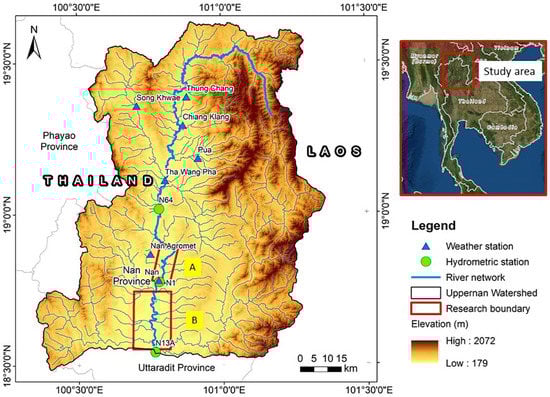
Figure 1.
Location map of Upper Nan Watershed. A: Muang Nan and B: Wiangsa.
Upper Nan Watershed is a fifth-order watershed, with an elongated shape, and is considered a rough watershed, with a drainage density of less than 2 km/km2, according to Smith [57]. The slope of this watershed is dominated by hilly (17–24%) and steep (25–35%) areas, which cover more than half of the watershed. Based on FAO [58], Upper Nan Watershed has four soil types: Orthic Acrisols (Ao90-2/3c), Ferric Acrisols (Af60-1/2ab), Orthic Acrisols (Ao108-2ab), and Dystric Nitosols (Nd65-3ab). The Orthic Acrisols (Ao90-2/3c) is the dominant soil type, which covers more than half of the total area.
The climate is tropical, with two distinct seasons: the dry season (from October to March) and the wet season (from April to September). It has an average annual rainfall of as much as 1385 mm. The average annual air temperature ranges between 4.5 °C and 43.3 °C. The annual flow at the watershed outlet (N13A station at Wiangsa) ranges between 29,765 and 158,033 m3/s.
According to the Land Development Department of Thailand, the majority of the land in the Upper Nan Watershed is forested, with an area of 5215.8 km2, followed by 25% dryland farming. Several previous studies have reported that deforestation and agricultural and built-up land encroachment is the main issue related to land use in this study area [59,60,61,62]. Moreover, these previous studies also report that the land use change in the study area led to several problems, such as increased streamflow fluctuation and sediment.
In this research, the study area inside Upper Nan Watershed was separated into two smaller areas, periodically inundated by flooding events: Muang Nan (A) and Wiangsa (B), as presented in Figure 1. Muang Nan, which covers 82 km2, is a study area located in the heart of economic activity in Nan Province. This area, located in the low-lying middle stream of Upper Nan, is supplied by discharge from the N64 station. Wiangsa is located downstream of Upper Nan Watershed. The N1 station supplies this area with a total area of 287 km2.
2.2. Data Collection
2.2.1. Topographic, Soil, and Land Use Data
The USGS DEM SRTM was used in this study to represent the topographic condition of the study area. This digital elevation model has a resolution of 30 m. These data were retrieved from Google Earth Engine (https://earthengine.google.com (accessed on 25 December 2021)).
In this study, we relied on the FAO digital soil map of the world for our soil data (DSMW). The DSMW was obtained from the United Nations Food and Agriculture Organization (https://www.fao.org (accessed on 11 January 2022)). These soil data have a 1:5,000,000 scale and cover the entire world, including the Upper Nan Watershed.
This study used a land use map of Upper Nan Watershed, created by Thailand’s Land Development Department. This study used a land use map from 2018, at a scale of 1:50,000 to emphasize the impact of climate change.
2.2.2. Hydro-Meteorological Data
Daily precipitation data from 1980 to 2020 were obtained from the Thai Meteorological Department (https://www4.tmd.go.th/ (accessed on 20 December 2021)). There are seven meteorological stations within Upper Nan Watershed: Nan, Nan Agromet, Tha Wang Pha, Thung Chang, Song Khwae, Chiang Klang, and Pua.
2.2.3. Discharge Data
Daily discharge data in this study were obtained from two different stations, managed by the Upper Northern Region Irrigation Hydrology Center, Royal Irrigation Department Thailand (www.hydro-1.net (accessed on 11 January 2022)). These stations are N64 (Baan Pakhwang) and N1 (Muang Nan). The data from each of these stations span a different number of years. Baan Pakhwang Station’s (N64) data cover April 1994–March 2022 and Muang Nan Station’s (N1) data cover April 1923–March 2021.
2.2.4. Observed Flood Map
The observed flood map was obtained from Thailand Flood Monitoring System, under Geo-Informatics and Space Technology Development (GISTDA), Thailand (https://flood.gistda.or.th (accessed on 3 March 2022)). The flood map provided by GISTDA has a scale of 1:5,000,000, which covers the entire country of Thailand. The observed flood map is available from 2005 to 2020 each month. However, the biggest flood in the study area occurred in 2008. Thus, this study used observed floods from this year only.
2.3. Model Description
2.3.1. SWAT Model
The SWAT model was created by The Agricultural Research Service of the USDA. It is a process-based, semi-distributed, continuous-time watershed hydrological model [63,64,65]. The SWAT model was developed to determine how management decisions affect water resources and pollution from non-point sources in large river basins [64]. Several data are required in the SWAT model: terrain, land use, soil, and meteorological data. Furthermore, multi-temporal observed discharge is also needed for calibration and validation requirements. Meteorological data include rainfall amount, air temperature, wind speed, solar radiation, and air humidity.
In this study, the SWAT model started by creating a delineated watershed and then separated it into multiple sub-watersheds, based on terrain data. The second step was to make the hydrologic response unit (HRU), which used land use, soil type, and slope data. Land use types from the Land Development Department, Thailand, were reclassified into nine major land use types: rice fields, built-up areas, dryland farming, forests, shrub grasses, water bodies, and miscellaneous. According to the DSMW map from FAO, there are four soil types in the study area. The slope in the study area is separated into five slope classifications: flat (0–8%), sloping (9–16%), hilly (17–24%), steep (25–35%), and very steep (>35%).
A water balance equation was the basis for the SWAT model [46,49]. The equation used in the SWAT model can be seen in Equation (1), as follows:
where SWt is the final soil water content (mm); SW0 is the initial soil water content (mm); t is the time (days); Rday is the rainfall amount on the day (mm); Wseep is the seepage water amount on the day (mm); and Qgw is the return flow on the day.
In the SWAT model, the Soil Conservation Service Curve Number (SCS-CN) method was applied to calculate the surface runoff in the study area. The SCS-CN equation is shown by Equation (2), as follows:
where Qsurf is daily surface runoff (mm); Rday is daily rainfall depth (mm); Ia is the initial abstraction (mm); and S is the retention parameter (mm). The value of S, or the retention parameter, is not fixed. It can be varied by several parameters such as slope, soil, and land use management. Mathematically, the value of the retention parameter can be expressed as Equation (3), as follows:
where S is the retention parameter (mm), and CN is the curve number. The curve number value is between 0 and 100, with 100 representing no potential retention, and 0 representing an infinite potential retention [66].
2.3.2. HEC-RAS Model
For 1D and 2D unsteady river hydraulic calculations, sediment transport predictions, and assessments of water quality, many researchers have turned to the United States Army Corps of Engineers’ HEC-RAS model [66]. In this study, we focused solely on 2D flood inundation, even though this model can perform various tasks.
The HEC-RAS model requires several datasets, including terrain, land use, and unsteady discharge. This model uses the same terrain as the SWAT model, a DEM SRTM with a 30 m resolution. In this model, land use defines the land surface’s manning value or the coarse level. The result of the SWAT model is an unsteady discharge.
A mesh or grid represents the terrain as a continuous surface in a 2D flood model. The water in this model can move through the mesh in longitudinal and lateral directions. In this study, a 50 × 50 m grid was used for the perimeter area, while the refinement area in the river valley and the area next to it used a 10 × 10-meter grid. These grids are generated in the RAS Mapper of HEC-RAS.
2.3.3. Coupled SWAT Model and HEC-RAS Model
SWAT model has been widely used in predicting the streamflow under various climatic and HRU conditions, whereas HEC-RAS 2D model has been widely used in river flood analyses. In this study, we used the versatility of these two models to predict the flood hazards that will occur in the study area as a result of climate change. The coupled SWAT and HEC-RAS model scheme used in this research is indicated in Figure 2.
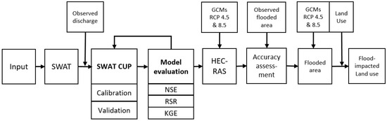
Figure 2.
Procedure for flood analysis using a coupled model, under climate change conditions.
2.4. Model Setup
2.4.1. SWAT Model
This study used two small areas within Upper Nan Watershed: Muang Nan and Wiangsa. The SWAT model setup in each of these study areas is described as follows:
- (1)
- Muang Nan (N64): This study area was divided into 29 sub-watersheds and 1414 HRUs. Data available for Muang Nan are from 1990 to 2020. Using the available data, the SWAT model was set up with a warm-up period of 5 years, calibration for 15 years, and validation for 11 years.
- (2)
- Wiangsa (N1): This study area was divided into 25 sub-watersheds and 1437 HRUs. Data available for Wiangsa were from 1980 to 2020. Using the available data, the SWAT model was set up with a warm-up period of 5 years, calibration for 20 years, and validation for 14 years.
SWAT model for all study areas was run by monthly time step for calibration and validation, then by daily time step for the input of the HEC-RAS model. SWAT model was run for the input of the HEC-RAS model using the maximum hydro-meteorological data available for the study area (from 1980 to 2020), with a warm-up period of five years.
2.4.2. HEC-RAS Model
The flood map in this study is generated by using HEC-RAS 2D model based on the SWAT-modelled streamflow. DEM SRTM, with a resolution of 30 m, was the input for terrain data. For the HEC-RAS model, the size of the area used was not the same as the size of the SWAT model’s area. This study emphasized the historically flooded area, based on the flood observation map from GISTDA. This was much smaller than the SWAT model area. The HEC-RAS study areas for Muang Nan and Wiangsa were 82.1 km2 and 286.98 km2, respectively.
All two study areas were covered by a 50 × 50 m grid perimeter area and a 10 × 10 m grid refinement area for the river valley and the area next to it. Manning information for this HEC-RAS model was based on the 2018 land use map, obtained from the Land Development Department of Thailand. This land use map was updated using 2021 Google Earth satellite imagery to improve the data updates and geometry. This study used a manning value based on Chow [67], Jung et al. [68], and Jansen [69]. This manning value was divided into normal, minimum, and maximum. This group was selected for calibrating the flood inundation model.
Each study area had different inputs. Muang Nan obtained input from Baan Pakhwang Station (N64), and Wiangsa obtained input from Muang Nan Station (N1). The input discharge in this study consisted of the following five groups:
- (1)
- August 2018, daily discharge.
- (2)
- Historical (1980–2020), daily discharge by using the return period.
- (3)
- Future (2021–2080), daily discharge by using the return period.
- (4)
- Future (2021–2080), daily discharge by using maximum flood in the near future (2025–2040), medium future (2041–2060), and far future (2061–2080).
The return period analysis in this study was based on the Log Pearson Type-III flood frequency method [70,71]. The return periods used in this study were 1, 2, 5, 10, 20, 50, and 100 years.
2.5. Model Evaluation
2.5.1. SWAT Model
A SWAT model should go through three processes before it is fit to use. These three processes are sensitivity analysis, calibration, and validation. Measures of sensitivity and significance, such as the t-value and the p-value, are applied to each parameter. The null hypothesis is rejected if the p-value is less than 0.05. In this study, a parameter with a high t-value and a low p-value was considered highly sensitive to streamflow changes [72,73].
The Nash–Sutcliffe efficiency (NSE) index, the RMSE-observations standard deviation ratio (RSR), and Kling–Gupta Efficiency (KGE) were selected in our study to evaluate the model’s monthly discharge performance at the calibration and validation phases. The RSR is the ratio of the measured data’s RMSE and standard deviation (Equation (4)). RSR ranges from 0 (optimal) to a large positive value. A lower RSR and RMSE improves model simulation performance [74]. NSE compares simulated and measured values to assess model efficiency, expressed in Equation (5) [75]. Model validity increases when NSE approaches 1 [76]. Calibration issues can develop when utilizing the commonly used NSE or the un-normalized mean square error criterion. Gupta et al. [77] introduced the KGE to lessen these issues. KGE values vary from −∞ to 1, with values closer to 1 suggesting a more effective model [78].
With α = σs/σo and β = μs/μo
Oi and Si are the observed and simulated values, n is the number of pairs, Ō is the mean observed value, and S is the mean simulated value. In this study, monthly NSE and RSR were deemed satisfactory based on performance rating statistics suggested by Moriasi et al. [79]. The NSE value of the model should be more than 0.50, while the RSR should not be more than 0.7. KGE can be categorized as good (KGE ≥ 0.75), intermediate (0.75 > KGE ≥ 0.5), poor (0.5 > KGE > 0), and very poor (KGE ≤ 0) [78].
2.5.2. HEC-RAS Model
An HEC-RAS-modelled flood needs to be evaluated to choose the best combination and understand the per cent error of the model. In this study, the HEC-RAS model was evaluated using a per cent accuracy assessment, by comparing the observed floods from the GISTDA- and HEC-RAS-modelled flood. According to the GISTDA flood database, the floods in the study area mostly occurred in August 2018. Thus, it was selected to examine the accuracy of the modelled flood.
This study’s parameters were chosen to vary the flood date and manning value. The flood date was chosen by the peak of the hydrograph, found during August 2018. The manning value had three categories: low, normal, and high. The combination of the flood on the selected date and the selected manning value categories was then used to generate the flood, using the HEC-RAS model. After that, the flood area was extracted using 50 × 50 m fishnet grids. The per cent accuracy assessment (A) was calculated using Equation (7), as follows:
where M is match which is the condition if the fishnet point (FP) from the observed flood and the modelled flood show the same condition, which can be all flooded or not flooded. The total numbers of fishnet points in Muang Nan and Wiangsa were 32,178 and 114,113 grid cells, respectively.
2.6. Future Climate Change Projection
This study used climate projection based on three GCMs in CMIP5, under the RCP4.5 and RCP8.5 scenarios: EC-Earth, HadGEM2, and MPI-ESM-MR, from 2006 to 2080. Climate data from 2006 to 2020 was used to select the most fitting GCM, which was able to predict future rainfall, streamflow, and flooded areas in our study area. Under Representative Concentration Pathway (RCP) 4.5, radiation forcing was seen to stabilize at 4.5 W m−2, (650 ppm CO2-equivalent) in 2100 [80]; therefore, we considered this RCP to be a future climate projection with a moderate impact. However, we consider Representative Concentration Pathway (RCP) 8.5 to be a high-emission scenario, with a high impact on the future environment. This RCP was seen to have a radiative forcing of 8.5 W m−2 in 2100, which is the highest scenario projected to date [1,81].
2.7. Statistical Test
The statistical test in this research was used to analyze the differences among the groups. In this study, a t-test was used with the equation shown below (Equation (8)). t-tests compare two groups’ means. The t-test assumes the datasets are independent, normally distributed, and have similar variance within each group [82]. Since the population variance was not similar, this study used a t-test for two samples, assuming unequal variances. We used a two-tailed t-test to compare populations, as follows:
Here, t is the t-value; x1 and x2 are the means of the two groups being compared; s2 is the pooled standard error of the two groups; and n1 and n2 are the numbers of observations in each group. This study employed a confidence interval of 95% or an alpha of 0.05. Two groups were considered significantly different if P(T ≤ t) was less than alpha.
3. Results
3.1. Future Precipitation
Precipitation is the input of a watershed. Understanding how the rainfall characteristics in our study area will change in the future as a result of climate change is crucial.
3.1.1. Selecting the Fittest GCM
In this study, we used three GCMs of CMIP5: EC-Earth, HadGEM2, and MPI-ESM-MR, under RCP4.5 and RCP8.5 scenarios. However, this study did not use all the GCMs to predict future streamflow and flooding. Instead, we only used the projection models that were suitable for the study area. The most suitable GCMs were chosen by comparing the minimum deviation from the observed rainfall with the projected rainfall between 2006 and 2020 (Table 1). As shown in Table 1, the minimum deviation was found in the MPI-ESM-MR’s dataset. Thus, this study only used a single GCM—MPI-ESM-MR—for the rest of the study.

Table 1.
Total deviation of GCMs value, compared to historical data.
3.1.2. Change in Rainfall Characteristics
The historical rainfall in the study area, between 1980 and 2020, showed particular features. The monthly rainfall showed that the wet season occurred in the middle of the year (between April and September), while the rest of the year was the dry season. The peak rainfall was seen to be in August, with a depth of as much as 309.4 mm. The annual rainfall was seen to fluctuate year-on-year; however, a rising tendency was observed. The average annual rainfall in the study area was seen to be 1385 mm, with a maximum rainfall of as much as 1957 recorded in 1995.
According to our projections, in the future, our study area will be wetter in both the dry and wet seasons. As shown in Figure 3a, our rainfall projections under RCP4.5 and RCP8.5 tended to predict more rainfall. In the dry season, we predict that the rainfall will increase by as much as 84% under RCP4.5 and by 83% under RCP8.5. Meanwhile, in the wet season we predict that under RCP4.5 and RCP8.5, the future rainfall will increase by as much as 11% and 10%, respectively. However, we do not predict any pattern changes in future rainfall: the dry season will still occur at the beginning and the end of the year, and the peak rainfall will still occur in August. Nevertheless, we predict the rainfall peak value under RCP4.5 to increase by as much as 4%; whereas, under RCP8.5, we predict it to decrease by 2%.
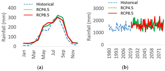
Figure 3.
Comparison of historical and future projections in Upper Nan Watershed: (a) monthly rainfall and (b) annual rainfall.
Similar to the monthly rainfall, we predict that the future annual rainfall will increase by as much as 19% under RCP4.5, and by 18% under RCP8.5 (Figure 3b). We predict the average annual rainfall under RCP4.5 and RCP8.5 to be 1650 mm and 1639 mm, respectively. Unlike the annual historical rainfall, we predict that future rainfall will fluctuate more. The rainfall projections under RCP4.5 and RCP8.5 had standard deviation values of as much as 281.9 and 261.2, respectively, while the historical rainfall only had a standard deviation value of 210.8.
In order to clarify the difference between the historical rainfall levels and our predicted future rainfall levels, we used t-test statistics in this study. As seen in Table 2, our future rainfall predictions were proven to have significant statistical differences under RCP4.5 and RCP8.5.
Table 2.
Statistical difference test among different rainfall conditions at Upper Nan Watershed.
3.2. Future Streamflow
The results of our study proved that climate change will significantly affect future rainfall in the Upper Nan Watershed. The next point that needed to be assessed was whether the streamflow would also be affected significantly. Thus, this part of the paper will highlight the effects of climate change on the streamflow within our research area and the future rainfall–runoff ratio.
3.2.1. Parameter Sensitivity, Calibration, and Validation
In order to model the future streamflow, the SWAT model needed to pass the sensitivity analysis, calibration, and validation. For the SWAT model at the N1 and N64 stations, we settled on eighteen parameters for calibration. Both the t-stat and the p-value were used to establish the sensitivity of the parameters [63,83]. The most sensitive parameters in each station were varied, as presented in Table 3.
Table 3.
Sensitive parameters for N1 and N64 stations.
The calibration and validation phase in SWAT model development relies on the observed streamflow [64,72]. The two stations, N1 and N64, had different periods of observation data available. The observation data from the N1 station were from between 1980 and 2020, while the data from the N65 station were from between 1990 and 2020. Therefore, the model configuration for the N1 station and N64 station was different. As shown in Figure 4a,b, the calibrated SWAT model at the N1 station and N64 station followed the pattern of the observed data well. This study used the NSE, RSR, and KGE values for the statistical evaluation. During the calibration and validation periods, both runoff stations had a good or very good NSE value—above 0.75. The RSR values, the calibration, and validation periods for stations N1 and N64 indicate satisfactory to very good values. Validation of N1 and calibration of N64 reveal intermediate KGE values, while calibration of N1 and validation of N64 show poor category.
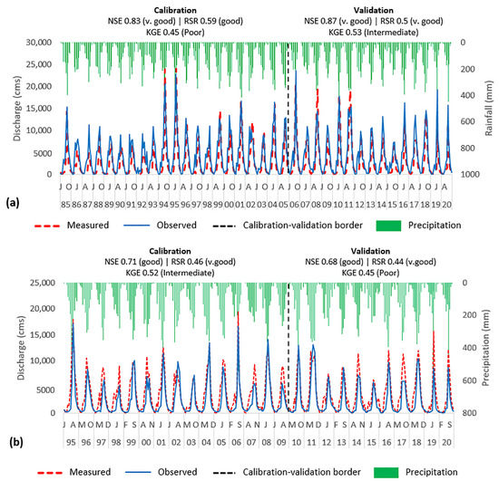
Figure 4.
Monthly time step: simulated and observed hydrograph at (a) N1 (Muang Nan Station) and (b) N64 (Ban Pakwang Station), with calculated statistics on calibration and validation periods.
3.2.2. Effect of Climate Change on Streamflow
The SWAT-modelled streamflow in this study used input from two sources: (1) the historical-modelled streamflow, which used the observed rainfall; and (2) the future-modelled streamflow, which used the MPI-ESM-MR, under RCP4.5 and RCP8.5 scenarios. The monthly historical streamflow was similar to the historical rainfall (Figure 5a). A low discharge was found at the beginning and the end of the year, while the peak discharge was found in August, with the values at the N1 and N64 stations as much as 12,260 m3/s and 9664 m3/s, respectively. The average annual streamflow of the historical period at the N1 and N64 stations was found to be as much as 51,538 m3/s and 40,869 m3/s, respectively. Meanwhile, the maximum discharge at N1 and N64 was 79,148 m3/s and 61,948 m3/s, respectively.
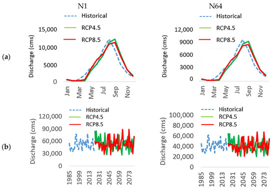
Figure 5.
Variation of streamflow, both historical and forecast, in Upper Nan Watershed at (a) monthly discharge and (b) annual discharge.
The predicted future monthly discharges showed a similar pattern as the historical streamflow. However, the future discharge had a one-month lag in the peak discharge compared to the historical streamflow. In the N1 station, the peak future discharge under RCP4.5 and RCP8.5 was lower by 7.7% and 11.9%, respectively, compared to the historical streamflow. In the N64 station, the peak future discharge under RCP4.5 and RCP8.5 was lower by 4.1% and 11.2%, respectively, compared to the historical streamflow. Furthermore, our predictions of the monthly future streamflow indicated that the dry season would be 43% wetter under RCP4.5 and 36% wetter under RCP8.5 at the N1 station, and 35.9% wetter under RCP4.5 and 29.3% wetter under RCP8.5 at the N64 station. Conversely, our predictions also showed that the wet season would be dryer by as much as 4.8% under RCP4.5 and by 2.4% under RCP8.5 in the N1 station, and by 8.4% under RCP4.5 and by 6% under RCP8.5 in the N64 station. This result corresponds with the study conducted by Tabucanon et al. [30]. Tabucanon et al. find that in the dry season under RCP4.5 and RCP8.5, streamflow in Chao Phraya’s tributary was predicted to increase, while the opposite occurred in the wet season.
Furthermore, according to our predictions, the future annual discharges also had a higher average, compared to the historical period. In the N1 station, we predicted the average annual discharge to be as much as 53,829 m3/s under RCP4.5, and 54,148 m3/s under RCP8.5. Meanwhile, in the N64 station, the average annual discharge was predicted to be as much as 41,001 m3/s under RCP4.5, and 41,244 m3/s under RCP8.5.
In order to clarify the difference between the historical and future streamflows, this study used t-test statistics. Using the value of the streamflow, the future streamflow was predicted to increase by between 0.3% and 5.1%, annually. However, the t-test analysis (shown in Table 4) found no significant difference between the future discharge and the historical discharge, even though the future rainfall was seen to be statistically different from the historic rainfall. This result is in line with a study conducted by Promping and Tingsanchali [55] which found that under RCP4.5, annual streamflow in Upper Nan Watershed was not significantly changed.
Table 4.
Statistical difference test among different streamflow conditions in N1 and N64 stations at Upper Nan Watershed.
3.3. Effect of Climate Change on Flood Events
In this study, we proved that climate change will affect the input of the Upper Nan Watershed. In order to further understand the effects of climate change on flood events, this section of the paper will explain the flood probability in the near future to the far future, changes in the flooded area, and the floods’ impact on the land use in our study area.
3.3.1. Model Evaluation
In order to choose the best model setup and understand the flood model’s accuracy, this study incorporated model evaluation, using accuracy assessment. Our accuracy assessment was based on the per cent matching of the observed flood and the modelled flood, according to a 50 × 50 m fishnet in the study area (shown in Table 5).
Table 5.
HEC-RAS model evaluation.
The results of the model evaluation in all of our study areas within the Upper Nan Watershed showed that the accuracy of the flood model was more than 80%. The highest accuracy was shown in Muang Nan—at 91.8%—while Wiangsa showed the lowest— 87.2%. Furthermore, the results showed that each study area’s manning range was best when used differently. This manning range was used in each study area, separately, to model the historical and future flood areas.
3.3.2. Flood Probability
In this particular study area, a flood is a recurrent event. According to probability, bigger floods occur less often than smaller ones. As shown in Figure 6, we found that the highest probability of a flood occurring was under the return period (RP) of 1 year, while the lowest probability was under the return period of 100 years.
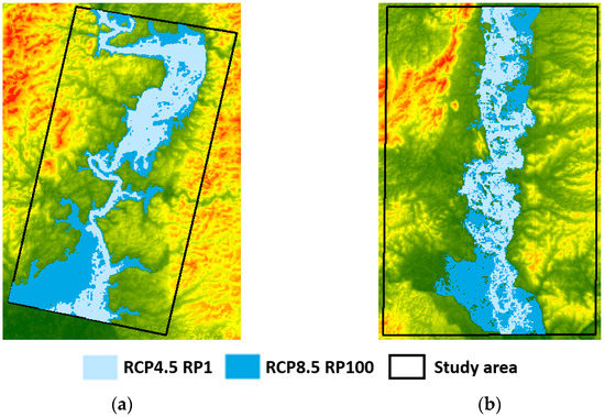
Figure 6.
Future flood extent of 1–100 years flood probability, under RCP4.5 and RCP8.5: (a) Muang Nan/N64 and (b) Wiangsa/N1.
The spatial extent of the flooded areas under the highest and lowest probability of a flood in both of the study areas (shown in Figure 6) had an obvious difference. In Muang Nan (N64), the area impacted by flooding under scenario RCP4.5, at a 1-year return period, was as large as 13.3 km2. As the size of the impacted area decreased, the probability of flooding in the area increased. Under the lowest probability under the RCP4.5 scenario that we calculated in this study—100 years—we predicted that the flood would impact an area as large as 26.5 km2. The same pattern was found in scenario RCP8.5, with the highest flood probability (RP1) affecting 14.3 km2, whereas the lowest flood probability (RP100) would potentially affect 27.6 km2. Similarly, in Wiangsa (N1), the same pattern was also observed. Under RCP4.5 and RCP8.5, from the highest probability (RP1) to the lowest probability (RP100), the flooding was predicted to affect as much as 32.1 km2, 64 km2, 33.9 km2, and 66.7 km2, respectively.
3.3.3. Flooding in Near Future, Medium Future, and Far Future
The MPI-ESM-MR projection projects the climate until the end of the 21st century. Due to this, it is possible to predict the future climate and its impact, including floods. As mentioned by Punyawasiri et al. [26], the future climate conditions can be broken down as follows: the near future (NF), from 2025 to 2040; the medium future (MF), from 2041 to 2060; and the far future (FF), from 2061 to 2080.
Our predictions of the flooding in the near future (NF), medium future (MF), and far future (FF) in Muang Nan and Wiangsa are presented in Figure 7. As seen in Figure 7, in all scenarios and in both locations, the flooding in the area will be the worst in the medium future period (2041–2060). In the Muang Nan (N64) location, the areas predicted to be submerged by flooding events in the medium future, under RCP4.5 and RCP8.5, are 26.3 km2 and 28.9 km2, respectively. While in the Wiangsa (N1), the flooded area in the medium future, under RCP4.5 and RCP8.5, was predicted to be as large as 61.6 km2 and 69.6 km2, respectively.
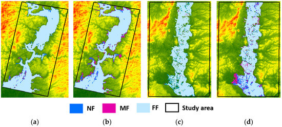
Figure 7.
Future extent of flooding in the medium future (2041–2060), under RCP4.5 and RCP8.5: (a) Muang Nan, RCP4.5; (b) Muang Nan, RCP8.5; (c) Wiangsa, RCP4.5; and (d) Wiangsa, RCP8.5.
3.3.4. Change in Flooded Area
We predict that the future floods in the Upper Nan Watershed will have more inundated areas, compared to the historical period studied. As presented in Table 6, we predict that future floods will inundate between 12.5% and 37.3% more of the area in Muang Nan. In Wiangsa, we predict that flooding will affect between 2.7% and 10% more of the area. We predict that the highest flood probability (RP1) in Muang Nan, under RCP4.5 and RCP8.5, will cover 12.5% and 20.6% more of the area, respectively. Meanwhile, in Wiangsa, we predict that the flooded area under RCP4.5 will decrease by 2.8%; whereas, under RCP8.5, we predict that the flooded area will increase by 2.7%.
Table 6.
Per cent difference between the flooded areas in historical floods and future flood predictions, under RCP 4.5 and RCP 8.5.
3.3.5. Impact on Land Use
Flood events, both directly and indirectly, impact the use of the land that is inundated by excess water. The future flood events that we have predicted in this study would inundate various land use types in our specific study areas. By overlaying the spatial flood extent with the land use map provided by Land Development of Thailand, 2018, with the adjustments made by using 2021 Google Earth imagery, we revealed the land uses that would be impacted by the flood events in both study areas.
In Muang Nan (N64), the three most impacted land use types would be tree plantations (TPs), between 3.9 and 6.8 km2 of this land would be affected; built-up areas (BAs), between 2.6 and 8.9 km2 of this land would be affected; and rice fields (RFs) between 1.8 and 3.1 km2 of this land would be affected. In Wiangsa (N1), the three most impacted land use types would be rice fields (RFs), between 9.4 and 25.5 km2 of this land would be affected; intercrop trees (ITs), between 8.4 and 15.3 km2 of this land would be affected; and built-up areas (BAs), between 3.1 and 11.1 km2 of this land would be affected. The total area that would be impacted by flooding among these three land use types, both in Muang Nan and Wiangsa, would be more than half of the total flooded area. The rest of the land use types impacted by the flood—such as dryland farming, forests, shrub grasses, water bodies, and miscellaneous—would account for a total of approximately 20% of the total flooded area.
4. Discussion
4.1. Change in Rainfall Characteristics
This study showed that the future rainfall will be significantly different from the historic rainfall. In the future, we predict that the Upper Nan Watershed will be wetter and have a high rainfall fluctuation. An increase in the amount of rainfall has already occurred in Thailand, as we can see by comparing the rainfall in the historical period with the rainfall today. A study conducted by Thailand’s Meteorological Department mentioned that between 1980 and 2021, the rainfall nationwide in Thailand has shown an increasing trend in the northern part of Thailand, including in the study area.
The future rainfall in the Upper Nan Watershed, as predicted by the MPI-ESM-MR, under the scenarios RCP4.5 and RCP8.5, will continue to increase until the end of the 21st century. The results of this study were in line with previous studies, conducted by Komori et al. [6] and Nontikansak et al. [84]. Both of these previous studies revealed that, according to future climate predictions, extreme rainfall will occur more frequently and with more intensity in most areas of Thailand.
The increase in the amount and intensity of rainfall and extreme events (as defined by IPCC [85]) will be a result of the increase in the global temperature, which is intensifying the global water cycle. Hotter air temperatures are accelerating evaporation in the water bodies, such as oceans and seas. However, the increase in surface temperature does not occur evenly in all locations, globally. Instead, surface temperatures are becoming hotter in some places and less hot in others. Under these conditions, the wind will become even stronger than it is at present, which will bring the water vapor from high-pressure areas to lower-pressure areas such as Southeast Asia. As predicted by IPCC [85], Southeast Asia will be one of the regions in the world that experiences more precipitation in the future.
Furthermore, the region of Southeast Asia, including Thailand, is frequently affected by tropical cyclones in the South China Sea and the Andaman Sea. According to Vongvisessomjai [86], Thailand is mostly affected by moderate north-westerly cyclone tracks in the rainy season. This phenomenon brings abundant water to Thailand and pours down in the Upper Nan Watershed, the first watershed in Thailand that faces the storm. Moreover, the orientation of this watershed is perpendicular to the tropical cyclone path, which leads to the occurrence of orographic rainfall by the watershed ridge. It is predicted that these tropical cyclones will intensify due to the increased temperature and air pressure differences worldwide, which will bring more rainfall to the Upper Nan Watershed.
4.2. Effect on Future Streamflow
This study discovered that the streamflow at both stations (N1 and N64) is not currently significantly different. However, the annual streamflow is predicted to increase in the future. Furthermore, the monthly streamflow peak is predicted to have a one-month lag, even if the future peak rainfall does not come one month later. Even if the rainfall, as the input of the study area, is significantly increased, it will not automatically lead to a significant rise in streamflow in the future.
Based on the principle of the hydrologic cycle in the watershed, some of the rainfall will be stored first in several places—such as the leaves of the plants; in the unsaturated zone, as soil moisture; and even stored further in the saturated zone, as groundwater. However, much of the excess rainfall water will flow from the watershed system as surface runoff. The lag time between the occurrence of the rainfall and the streamflow reaching the outlet of the watershed could explain the one-month lag in the predicted future streamflow peak.
The future rise in the streamflow that was predicted in this study was also confirmed by previous studies conducted in the same region. These were studies by Kure and Tebakari [87], Tabucanon et al. [30], and Hunukumbara and Tachikawa [88]. Kure and Tebakari explained that, under scenario A1B of SRES, using MRI atmospheric general circulation models 3.1 and 3.2, the mean annual river discharge is expected to increase in the Chao Phraya River Basin. Furthermore, a study by Tabucanon et al. in Bhumibol Dam, Ping River, Northern Thailand, found that under EC-EARTH, the discharge inflow to the dam will experience enormous fluctuation, especially in the wet season. In another study by Hunukumbara and Tachikawa, it was discovered that the predicted discharge will increase both in the near future (2015–2039) and in the far future (2075–2099) in the north-central and the south-western parts of the Chao Phraya Watershed.
4.3. Effect on Future Flood Events
Both Muang Nan and Wiangsa are situated in the intermontane basin, a low-lying floodplain valley, surrounded by a mountainous area. A steep slope with high drainage density characteristics makes the study area prone to flash floods, since the streamflow rapidly accumulates downstream, in the lowest part of the watershed. Thus, the spatial flood pattern in this particular study area follows the low-lying, flat-sloped floodplain around the river. Muang Nan has more flat areas, which is why the extent of the floods in Muang Nan is larger than in Wiangsa.
It is still necessary to consider mitigation efforts before the actual floods occur in the far future, as part of the disaster risk reduction; however, we also need to be cautious and prepared in the medium future (2041–2060) for a flood in Muang Nan, under both RCP4.5 and RCP8.5. This flood is more likely to be of the same magnitude as that calculated for the 100-year flooding probability. The medium future flood of Wiangsa, under RCP4.5, is more likely to be of the same magnitude as that calculated for the 50-year flood probability, whereas the flood under RCP8.5 is likely to be of a similar magnitude to that calculated for the 100-year flood probability. Furthermore, the flooding of Muang Nan and Wiangsa, under both RCP4.5 and RCP8.5, in the near future (2025–2040), is predicted to be of a similar magnitude to the 50-year flood probability. Compared to the flood probabilities, the far future flood (2061–2080) is one that we should worry less about since the magnitude is only predicted to be similar to the 10–20-year flood probability.
Several of the areas that we predict will be inundated are considered vast, and possibly produce a huge amount of rice, which is a staple food for the local community and for neighboring countries. This study revealed that the three most impacted land uses in the study area will be rice fields, built-up areas, and intercrop trees. Of these three types of land use, the rice field will be the most largely impacted. In summation, in Muang Nan and Wiangsa, the area of rice fields that will potentially be impacted by the least frequent flood probability, at a return period of 100 years, could be as much as 28.5 km2. This number is 138.2% higher than the most common of the predicted flood probabilities (1-year flood).
The inundation of rice fields after a flood event in Thailand has been reported several times in previous studies. These reports are mostly from the 2011 flood since it was the worst flood that has been experienced in the modern period. Son et al. [89] reported that, due to the 2011 flood in Thailand, 16.8% of the rice cultivation area in the Chao Phraya River Delta, which is dominated by land used for double-cropped rice, was inundated by flood water, causing damage to the rice. Similarly, Kotera et al. [90], also reported on the same flood event, stating that at least 52.3% of the inundated area was categorized as damaged. Furthermore, Nara et al. [91] mentioned that, due to the 2011 flood event, Thailand reported experiencing an economic slowdown because it had lost a considerable amount of rice, which is its major export commodity.
The great flood of 2011, in Thailand, caused a considerable amount of disruption. As it is, this flood will continue to be used as a reference point for the worst flood event in Thailand. Although we predict that floods will occur in the near future (2025–2040), we predict that the worst will occur in the middle future (2041–2060); therefore, we need to monitor the situation closely and prepare for it very well to reduce our potential losses in the future and avoid the considerable disruption that we experienced as a result of the 2011 flood.
5. Conclusions
The impacts of climate change in Thailand varied between the regions. The northern part of Thailand, represented by the Upper Nan Watershed, is predicted to be significantly impacted by climate change. Our study revealed that the rainfall in the Upper Nan Watershed, which has already shown an increasing trend, is predicted to increase further due to climate change. This will lead to a wetter Upper Nan Watershed in the future, both in the dry and wet seasons. Furthermore, increasing rainfall will change the characteristics of future discharge in the area. The change in the characteristics of the future discharge, such as the one-month delay in the timing of the discharge peak, the annual amount of the discharge peak increasing from 0.3% to 5.1%, and the discharge fluctuation. Moreover, this change in the discharge in the study area will increase the flooded area of land within the Upper Nan Watershed by between 12.5% and 37.3% in Muang Nan and between 2.7 and 10% in Wiangsa.
This study found that in the medium future (2041–2060), both Muang Nan and Wiangsa will potentially experience the magnitude of flooding associated with the 100-year flood probability. At the same time, we predict that the magnitude of flooding associated with the 50-year flood probability will also face these particular study areas in the near future (2025–2040). The rice field is the most common land use type in the area and, thus, will be the most impacted by these potential flood events. Therefore, it is essential that we closely monitor the situation and prepare well to reduce our potential losses in the future and avoid repeating the disruption that we experienced after the 2011 flood.
This study only focused on small and specific regions, so that the HEC-RAS model could focus more on the riverine flood modelling. However, floods that are caused by other phenomena, i.e., flash floods, were not covered. Furthermore, we did not discuss the best management practices (BMPs) for the watershed’s land use utilization and we did not consider the simulation of flood mitigation infrastructure (i.e., dikes, dams, gabions, and riparian zones) to reduce the impact of future floods. Therefore, we suggest that the next study should include a larger coverage area for the HEC-RAS model and that it should explore several BMPs and flood mitigation scenarios.
Author Contributions
Conceptualization, methodology, analysis, investigation, visualization, and writing—original draft, M.C.S.; supervision, review, and editing, P.T. and N.K. All authors have read and agreed to the published version of the manuscript.
Funding
This research was funded by DAAD and Southeast Asian Regional Center for Graduate Study and Research in Agricultural (SEARCA).
Institutional Review Board Statement
Not applicable.
Informed Consent Statement
Not applicable.
Data Availability Statement
Not applicable.
Acknowledgments
We thank the Thailand Meteorological Department for providing climatic data, including the down-scaled CMIP5 GCMs.
Conflicts of Interest
The authors declare no conflict of interest.
References
- Pörtner, H.-O.; Roberts, D.C.; Poloczanska, E.S.; Mintenbeck, K.; Tignor, M.; Alegría, A.; Craig, M.; Langsdorf, S.; Löschke, S.; Möller, V.; et al. Climate Change 2022: Impacts, Adaptation and Vulnerability Summary for Policymakers; Cambridge University Press: Cambridge, UK, 2022. [Google Scholar] [CrossRef]
- Held, I.M.; Soden, B.J. Robust Responses of the Hydrological Cycle to Global Warming. J. Clim. 2006, 19, 5686–5699. [Google Scholar] [CrossRef]
- Trenberth, K.E. Changes in precipitation with climate change. Clim. Res. 2011, 47, 123–138. [Google Scholar] [CrossRef]
- Petpongpan, C.; Ekkawatpanit, C.; Bailey, R.T.; Kositgittiwong, D.; Saraphirom, P. Evaluating Surface Water-groundwater Interactions in Consequence of Changes in Climate and Groundwater Extraction. Water Resour. Manag. 2022, 36, 5767–5783. [Google Scholar] [CrossRef]
- Gunathilake, M.B.; Amaratunga, Y.V.; Perera, A.; Chathuranika, I.M.; Gunathilake, A.S.; Rathnayake, U. Evaluation of Future Climate and Potential Impact on Streamflow in the Upper Nan River Basin of Northern Thailand. Adv. Meteorol. 2020, 2020, 1–15. [Google Scholar] [CrossRef]
- Komori, D.; Rangsiwanichpong, P.; Inoue, N.; Ono, K.; Watanabe, S.; Kazama, S. Distributed probability of slope failure in Thailand under climate change. Clim. Risk Manag. 2018, 20, 126–137. [Google Scholar] [CrossRef]
- Akpodiogaga-a, P.; Odjugo, O. General Overview of Climate Change Impacts in Nigeria. J. Hum. Ecol. 2010, 29, 47–55. [Google Scholar] [CrossRef]
- Almazroui, M.; Islam, M.N.; Athar, H.; Jones, P.D.; Rahman, M.A. Recent climate change in the Arabian Peninsula: Annual rainfall and temperature analysis of Saudi Arabia for 1978–2009. Int. J. Climatol. 2012, 32, 953–966. [Google Scholar] [CrossRef]
- Shen, G.; Hwang, S.N. Spatial–Temporal snapshots of global natural disaster impacts Revealed from EM-DAT for 1900–2015. Geomat. Nat. Hazards Risk 2019, 10, 912–934. [Google Scholar] [CrossRef]
- Farid, M.; Gunawan, B.; Syahril, M.; Kusuma, B.; Habibi, S.A. Assessment of flood risk reduction in Bengawan Solo river: A case study of Sragen Regency. Int. J. Geomate 2020, 18, 229–234. [Google Scholar] [CrossRef]
- Thamtanajit, K. The Impacts Of Natural Disaster On Student Achievement: Evidence From Severe Floods in Thailand. J. Dev. Areas 2020, 54. [Google Scholar] [CrossRef]
- Ozturk, U.; Wendi, D.; Crisologo, I.; Riemer, A.; Agarwal, A.; Vogel, K.; López-Tarazón, J.A.; Korup, O. Science of the Total Environment Rare flash floods and debris flows in southern Germany. Sci. Total Environ. 2018, 626, 941–952. [Google Scholar] [CrossRef]
- Tay, C.W.J.; Yun, S.-H.; Chin, S.T.; Bhardwaj, A.; Jong, J.; Hill, E.M. Rapid flood and damage mapping using synthetic aperture radar in response to Typhoon Hagibis, Japan. Sci. Data 2020, 7, 1–9. [Google Scholar] [CrossRef]
- Dottori, F.; Szewczyk, W.; Ciscar, J.-C.; Zhao, F.; Alfieri, L.; Hirabayashi, Y.; Bianchi, A.; Mongelli, I.; Frieler, K.; Betts, R.A.; et al. Increased human and economic losses from river flooding with anthropogenic warming. Nat. Clim. Chang. 2018, 8, 781–786. [Google Scholar] [CrossRef]
- Chokkavarapu, N.; Mandla, V.R. Comparative study of GCMs, RCMs, downscaling and hydrological models: A review toward future climate change impact estimation. SN Appl. Sci. 2019, 1, 1698. [Google Scholar] [CrossRef]
- Collins, M.; Chandler, R.E.; Cox, P.M.; Huthnance, J.M.; Rougier, J.; Stephenson, D.B. Quantifying future climate change. Nat. Clim. Chang. 2012, 2, 403–409. [Google Scholar] [CrossRef]
- Vecchi, G.A.; Wittenberg, A.T. El Niño and our future climate: Where do we stand? Wiley Interdiscip. Rev. Clim. Chang. 2010, 1, 260–270. [Google Scholar] [CrossRef]
- Ulbrich, U.; Leckebusch, G.C.; Pinto, J.G. Extra-tropical cyclones in the present and future climate: A review. Theor. Appl. Climatol. 2009, 96, 117–131. [Google Scholar] [CrossRef]
- Zscheischler, J.; Westra, S.; Van Den Hurk, B.J.J.M.; Seneviratne, S.I.; Ward, P.J.; Pitman, A.; AghaKouchak, A.; Bresch, D.N.; Leonard, M.; Wahl, T.; et al. Future climate risk from compound events. Nat. Clim. Chang. 2018, 8, 469–477. [Google Scholar] [CrossRef]
- Chen, C.A.; Hsu, H.H.; Liang, H.C. Evaluation and comparison of CMIP6 and CMIP5 model performance in simulating the seasonal extreme precipitation in the Western North Pacific and East Asia. Weather Clim. Extrem. 2021, 31, 100303. [Google Scholar] [CrossRef]
- Rojpratak, S.; Supharatid, S. Regional extreme precipitation index: Evaluations and projections from the multi-model ensemble CMIP5 over Thailand. Weather Clim. Extrem. 2022, 37, 100475. [Google Scholar] [CrossRef]
- Niu, Z.; Feng, L.; Chen, X.; Yi, X. Evaluation and future projection of extreme climate events in the yellow river basin and yangtze river basin in china using ensembled cmip5 models data. Int. J. Environ. Res. Public Health 2021, 18, 6029. [Google Scholar] [CrossRef] [PubMed]
- Wang, Z.; Han, L.; Zheng, J.; Ding, R.; Li, J.; Hou, Z.; Chao, J. Evaluation of the performance of CMIP5 and CMIP6 models in simulating the victoria mode-el niño relationship. J. Clim. 2021, 34, 7625–7644. [Google Scholar] [CrossRef]
- Deng, X.; Perkins-Kirkpatrick, S.E.; Lewis, S.C.; Ritchie, E.A. Evaluation of Extreme Temperatures Over Australia in the Historical Simulations of CMIP5 and CMIP6 Models. Earth’s Futur. 2021, 9, e2020EF001902. [Google Scholar] [CrossRef]
- Chen, H.; Sun, J.; Lin, W.; Xu, H. Comparison of CMIP6 and CMIP5 models in simulating climate extremes. Sci. Bull. 2020, 65, 1415–1418. [Google Scholar] [CrossRef]
- Punyawansiri, S.; Kwanyuen, B. Forecasting the Future Temperature Using a Downscaling Method by LARS-WG Stochastic Weather Generator at the Local Site of Phitsanulok Province, Thailand. Atmos. Clim. Sci. 2020, 10, 538–552. [Google Scholar] [CrossRef]
- Babel, M.S.; Sirisena, T.A.J.G.; Singhrattna, N. Incorporating large-scale atmospheric variables in long-term seasonal rainfall forecasting using artificial neural networks: An application to the Ping Basin in Thailand. Hydrol. Res. 2017, 48, 867–882. [Google Scholar] [CrossRef]
- Pattnayak, K.C.; Kar, S.C.; Dalal, M.; Pattnayak, R.K. Projections of annual rainfall and surface temperature from CMIP5 models over the BIMSTEC countries. Glob. Planet. Chang. 2017, 152, 152–166. [Google Scholar] [CrossRef]
- Pomoim, N.; Zomer, R.J.; Hughes, A.C.; Corlett, R.T. The sustainability of thailand’s protected-area system under climate change. Sustainability 2021, 13, 2868. [Google Scholar] [CrossRef]
- Tabucanon, A.S.; Rittima, A.; Raveephinit, D.; Phankamolsil, Y.; Sawangphol, W.; Kraisangka, J.; Talaluxmana, Y.; Vudhivanich, V.; Xue, W. Impact of climate change on reservoir reliability: A case of bhumibol dam in ping river basin, Thailand. Environ. Nat. Resour. J. 2021, 19, 266–281. [Google Scholar] [CrossRef]
- Ankit, P.C.; Sangam, S. Climate Change Impacts and Adaptation Strategies on Maize and Rice Yield in Nan River Basin, Thailand. In Proceedings of the AGU Fall Meeting Abstracts, New Orleans, LA, USA, 13–17 December 2021. [Google Scholar]
- Kyaw, K.M.; Rittima, A.; Phankamolsil, Y.; Tabucanon, A.S.; Sawangphol, W.; Kraisangka, J.; Vudhivanich, V. Assessing Reservoir Reoperation Performances through Adapted Rule Curve and Hedging Policies under Climate Change Scenarios: In--depth Investigation of Case Study of Bhumibol Dam in Thailand. Eng. Access 2022, 8, 179–185. [Google Scholar] [CrossRef]
- IPCC. Climate Change 2014 Synthesis Report Summary for Policymakers; IPCC: Cambridge, UK, 2014. [Google Scholar]
- Dukat, P.; Bednorz, E.; Ziemblińska, K.; Urbaniak, M. Trends in drought occurrence and severity at mid-latitude European stations (1951–2015) estimated using standardized precipitation (SPI) and precipitation and evapotranspiration (SPEI) indices. Meteorol. Atmos. Phys. 2022, 134, 1–21. [Google Scholar] [CrossRef]
- Daneshvar, M.R.M.; Ebrahimi, M.; Nejadsoleymani, H. An overview of climate change in Iran: Facts and statistics. Environ. Syst. Res. 2019, 8, 7. [Google Scholar] [CrossRef]
- Cheng, C.; Yang, Y.C.E.; Ryan, R.; Yu, Q.; Brabec, E. Assessing climate change-induced flooding mitigation for adaptation in Boston’s Charles River watershed, USA. Landsc. Urban Plan. 2017, 167, 25–36. [Google Scholar] [CrossRef]
- Kharel, G.; Zheng, H.; Kirilenko, A. Can land-use change mitigate long-term flood risks in the Prairie Pothole Region? The case of Devils Lake, North Dakota, USA. Reg. Environ. Chang. 2016, 16, 2443–2456. [Google Scholar] [CrossRef]
- Novelo-Casanova, D.A.; Rodríguez-Vangort, F. Flood risk assessment. Case of study: Motozintla de Mendoza, Chiapas, Mexico. Geomat. Nat. Hazards Risk 2016, 7, 1538–1556. [Google Scholar] [CrossRef]
- Boithias, L.; Sauvage, S.; Lenica, A.; Roux, H.; Abbaspour, K.C.; Larnier, K.; Dartus, D.; Sánchez-Pérez, J.M. Simulating flash floods at hourly time-step using the SWAT model. Water 2017, 9, 929. [Google Scholar] [CrossRef]
- Eingrüber, N.; Korres, W. Climate change simulation and trend analysis of extreme precipitation and floods in the mesoscale Rur catchment in western Germany until 2099 using Statistical Downscaling Model (SDSM) and the Soil & Water Assessment Tool (SWAT model). Sci. Total Environ. 2022, 838, 155775. [Google Scholar] [CrossRef]
- Urzică, A.; Mihu-Pintilie, A.; Stoleriu, C.C.; Cîmpianu, C.I.; Huţanu, E.; Pricop, C.I.; Grozavu, A. Using 2D HEC-RAS modeling and embankment dam break scenario for assessing the flood control capacity of a multireservoir system (Ne Romania). Water 2021, 13, 57. [Google Scholar] [CrossRef]
- Birhanu, D.; Kim, H.; Jang, C.; Park, S. Flood Risk and Vulnerability of Addis Ababa City Due to Climate Change and Urbanization. Procedia Eng. 2016, 154, 696–702. [Google Scholar] [CrossRef]
- Hounkpè, J.; Diekkrüger, B.; Afouda, A.A.; Sintondji, L.O.C. Land use change increases flood hazard: A multi-modelling approach to assess change in flood characteristics driven by socio-economic land use change scenarios. Nat. Hazards 2019, 98, 1021–1050. [Google Scholar] [CrossRef]
- Desalegn, H.; Mulu, A. Mapping flood inundation areas using GIS and HEC-RAS model at Fetam River, Upper Abbay Basin, Ethiopia. Sci. Afr. 2021, 12, e00834. [Google Scholar] [CrossRef]
- Liu, Y.; Xu, Y.; Zhao, Y.; Long, Y. Using SWAT Model to Assess the Impacts of Land Use and Climate Changes on Flood in the Upper Weihe River, China. Water 2022, 14, 2098. [Google Scholar] [CrossRef]
- Kartikasari, A.N.I.; Halik, G.; Wiyono, R.U.A. Land Use Scenario Modelling for Floods Mitigation in Bedadung Watershed, East Java Indonesia. J. Eng. Sci. Technol. 2022, 17, 2020–2034. [Google Scholar]
- Rohmat, F.I.W.; Sa’adi, Z.; Stamataki, I.; Kuntoro, A.A.; Farid, M.; Suwarman, R. Flood modeling and baseline study in urban and high population environment: A case study of Majalaya, Indonesia. Urban Clim. 2022, 46, 101332. [Google Scholar] [CrossRef]
- Prasanchum, H.; Sirisook, P.; Lohpaisankrit, W. Flood risk areas simulation using SWAT and Gumbel distribution method in Yang Catchment, Northeast Thailand. Geogr. Tech. 2020, 15, 29–39. [Google Scholar] [CrossRef]
- Wangpimool, W.; Pongput, K.; Supriyasilp, T.; Sakolnakhon, K.P.N. Hydrological Evaluation with SWAT Model and Numerical Weather Prediction for Flash Flood Warning System in Thailand. J. Earth Sci. Eng. 2013, 6, 349–357. [Google Scholar]
- Maskong, H.; Jothiyangkoon, C.; Hirunteeyakul, C. Flood Hazard Mapping Using on-Site Surveyed Flood Map, HECRAS V.5 and GIS Tool: A Case Study of Nakhon Ratchasima Municipality, Thailand. Int. J. Geomate 2019, 16, 1–8. [Google Scholar] [CrossRef]
- Roy, B.; Khan, M.S.M.; Islam, A.K.M.S.; Mohammed, K.; Khan, M.J.U. Climate-induced flood inundation for the Arial Khan River of Bangladesh using open-source SWAT and HEC-RAS model for RCP8.5-SSP5 scenario. SN Appl. Sci. 2021, 3, 1–13. [Google Scholar] [CrossRef]
- Loi, N.K.; Liem, N.D.; Tu, L.H.; Hong, N.T.; Truong, C.D.; Tram, V.N.Q.; Nhat, T.T.; Anh, T.N.; Jeong, J. Automated procedure of real-time flood forecasting in vu gia—Thu bon river basin, vietnam by integrating swat and hec-ras models. J. Water Clim. Chang. 2019, 10, 535–545. [Google Scholar] [CrossRef]
- Warren, R.; Arnell, N.; Nicholls, R.; Levy, P.; Price, J. Understanding the Regional Impacts of Climate Change. Tyndall Cent. Clim. Chang. Res. Work. Pap. 2006, 27–60, Working Paper 90. Available online: http://www.tyndall.ac.uk/publications/working_papers/twp90.pdf (accessed on 5 October 2022).
- Artlert, K.; Chaleeraktrakoon, C.; Van Nguyen, V.T. Modeling and analysis of rainfall processes in the context of climate change for Mekong, Chi, and Mun River Basins (Thailand). J. Hydro-Environ. Res. 2013, 7, 2–17. [Google Scholar] [CrossRef]
- Promping, T.; Tingsanchali, T. Effects of Climate Change and Land-use Change on Future Inflow to a Reservoir: A Case Study of Sirikit Dam, Upper Nan River Basin, Thailand. Gmsarn Int. J. 2022, 16, 366–376. [Google Scholar]
- Igarashi, K.; Koichiro, K.; Tanaka, N.; Aranyabhaga, N. Prediction of the Impact of Climate Change and Land Use Change on Flood Discharge in the Song Khwae District, Nan Province, Thailand. J. Clim. Chang. 2019, 5, 1–8. [Google Scholar] [CrossRef]
- Smith, K.G. Standards for grading texture of erosional topography. Am. J. Sci. 1950, 248, 655–668. [Google Scholar] [CrossRef]
- FAO. FAO Digital Soil Map of the World (DSMW). Available online: https://www.fao.org/land-water/land/land-governance/land-resources-planning-toolbox/category/details/en/c/1026564/ (accessed on 3 March 2023).
- Pakoksung, K.; Takagi, M. Effect of land cover change in runoff estimation on flood event; case study in the upper part area of Nan river basin, Thailand. In Proceedings of the 37th Asian Conference on Remote Sensing, ACRS 2016, Colombo, Sri Lanka, 17–21 October 2016; Volume 3, pp. 1788–1797. [Google Scholar]
- Koontanakulvong, S.; Pakoksung, K. Impact of Land Use Change on Runoff Volume in Upper Nan Basin Area. In Proceedings of the 2nd EIT International Conference on Water Resources Engineering, Chiangrai, Thailand, 5–6 September 2013. [Google Scholar]
- Paiboonvorachat, C.; Oyana, T.J. Land-cover changes and potential impacts on soil erosion in the nan watershed, Thailand. Int. J. Remote Sens. 2011, 32, 6587–6609. [Google Scholar] [CrossRef]
- Jirasirichote, A.; Ninsawat, S.; Shrestha, S.; Tripathi, N.K. Performance of AnnAGNPS model in predicting runoff and sediment yields in Nan Province, Thailand. Heliyon 2021, 7, e08396. [Google Scholar] [CrossRef]
- Li, C.; Fang, H. Assessment of climate change impacts on the streamflow for the Mun River in the Mekong Basin, Southeast Asia: Using SWAT model. Catena 2021, 201, 105199. [Google Scholar] [CrossRef]
- Arnold, J.G.; Moriasi, D.N.; Gassman, P.W.; Abbaspour, K.C.; White, M.J.; Srinivasan, R.; Jha, M.K. SWAT: Model Use, Calibration, and Validation. Am. Soc. Agric. Biol. Eng. 2012, 55, 1491–1508. [Google Scholar]
- Gassman, P.W.; Sadeghi, A.M.; Srinivasan, R. Applications of the SWAT Model Special Section: Overview and Insights. J. Environ. Qual. 2014, 43, 1–8. [Google Scholar] [CrossRef]
- Aawar, T.; Khare, D. Assessment of climate change impacts on streamflow through hydrological model using SWAT model: A case study of Afghanistan. Model. Earth Syst. Environ. 2020, 6, 1427–1437. [Google Scholar] [CrossRef]
- Chow, V.T. Open-Channel Hydraulics; McGraw Hill: New York, NY, USA, 1959. [Google Scholar]
- Jung, I.K.; Park, J.Y.; Park, G.A.; Lee, M.S.; Kim, S.J. A grid-based rainfall-runoff model for flood simulation including paddy fields. Paddy Water Environ. 2011, 9, 275–290. [Google Scholar] [CrossRef]
- Curtis, J. Manning’s n Values for Various Land Covers. To Use for Dam Breach Analyses by NRCS in Kansas, No. February, pp. 1–2, 2016. Available online: https://rashms.com/wp-content/uploads/2021/01/Mannings-n-values-NLCD-NRCS.pdf (accessed on 8 October 2022).
- Bobee, B.B.; Robitaille, R. The Use of the Pearson Type 3 and Log Pearson Type 3 Distribution Revisited. Water Resour. Res. 1977, 13, 427–443. [Google Scholar] [CrossRef]
- Kumar, R. Flood Frequency Analysis of the Rapti River Basin using Log Pearson Type-III and Gumbel Extreme Value-1 Methods. J. Geol. Soc. India 2019, 94, 480–484. [Google Scholar] [CrossRef]
- Abbaspour, K.C. SWAT-CUP: SWAT Calibration and Uncertainly Programs—A User Manual; Swiss Federal Institute of Aquatic Science and Technology, Eawag: Dübendorf, Switzerland, 2015. [Google Scholar] [CrossRef]
- Guo, J.; Su, X. Parameter sensitivity analysis of SWAT model for streamflow simulation with multisource precipitation datasets. Hydrol. Res. 2019, 50, 861–877. [Google Scholar] [CrossRef]
- Golmohammadi, G.; Prasher, S.; Madani, A.; Rudra, R. Evaluating three hydrological distributed watershed models: MIKE-SHE, APEX, SWAT. Hydrology 2014, 1, 20–39. [Google Scholar] [CrossRef]
- Gitau, M.W.; Chaubey, I. Regionalization of SWAT model parameters for use in ungauged watersheds. Water 2010, 2, 849–871. [Google Scholar] [CrossRef]
- Yang, M.; Xu, J.; Yin, D.; He, S.; Zhu, S.; Li, S. Modified Multi–Source Water Supply Module of the SWAT–WARM Model to Simulate Water Resource Responses under Strong Human Activities in the Tang–Bai River Basin. Sustainability 2022, 14, 15016. [Google Scholar] [CrossRef]
- Gupta, H.V.; Kling, H.; Yilmaz, K.K.; Martinez, G.F. Decomposition of the mean squared error and NSE performance criteria: Implications for improving hydrological modelling. J. Hydrol. 2009, 377, 80–91. [Google Scholar] [CrossRef]
- Towner, J.; Cloke, H.L.; Zsoter, E.; Flamig, Z.; Hoch, J.M.; Bazo, J.; de Perez, E.C.; Stephens, E.M. Assessing the performance of global hydrological models for capturing peak river flows in the Amazon basin. Hydrol. Earth Syst. Sci. 2019, 23, 3057–3080. [Google Scholar] [CrossRef]
- Moriasi, D.N.; Arnold, J.G.; Van Liew, M.W.; Bingner, R.L.; Harmel, R.D.; Veith, T.L. Model Evaluation Guidelines for Systematic Quantification of Accuracy in Watershed Simulations. Trans. ASABE 2007, 50, 885–900. [Google Scholar] [CrossRef]
- Thomson, A.M.; Calvin, K.V.; Smith, S.J.; Kyle, G.P.; Volke, A.; Patel, P.; Delgado-Arias, S.; Bond-Lamberty, B.; Wise, M.A.; Clarke, L.E.; et al. RCP4.5: A pathway for stabilization of radiative forcing by 2100. Clim. Chang. 2011, 109, 77–94. [Google Scholar] [CrossRef]
- Riahi, K.; Rao, S.; Krey, V.; Cho, C.; Chirkov, V.; Fischer, G.; Kindermann, G.E.; Nakicenovic, N.; Rafaj, P. RCP 8.5-A scenario of comparatively high greenhouse gas emissions. Clim. Chang. 2011, 109, 33–57. [Google Scholar] [CrossRef]
- Bevans, R. An Introduction to t Test: Definitions, Formula and Examples; Scribbr: Amsterdam, The Netherlands, 2022; Available online: https://www.scribbr.com/statistics/t-test/ (accessed on 18 December 2022).
- Tuo, Y.; Duan, Z.; Disse, M.; Chiogna, G. Evaluation of precipitation input for SWAT modeling in Alpine catchment: A case study in the Adige river basin (Italy). Sci. Total Environ. 2016, 573, 66–82. [Google Scholar] [CrossRef]
- Nontikansak, P.; Shrestha, S.; Shanmugam, M.S.; Loc, H.H.; Virdis, S.G.P. Rainfall extremes under climate change in the Pasak River Basin, Thailand. J. Water Clim. Chang. 2022, 13, 3729–3746. [Google Scholar] [CrossRef]
- Masson-Delmotte, V.; Barros, V.; Burton, I.; Campbell-Lendrum, D.; Cardona, O.-D.; Cutter, S.L.; Dube, O.P.; Ebi, K.L.; Field, C.B.; Handmer, J.W.; et al. Climate Change 2021: The Physical Science Basis Summary for Policymakers; Cambridge University Press: Cambridge, UK, 2021. [Google Scholar] [CrossRef]
- Vongvisessomjai, S. Tropical cyclone disasters in the Gulf of Thailand. Songklanakarin J. Sci. Technol. 2009, 31, 213–227. [Google Scholar]
- Kure, S.; Tebakari, T. Hydrological impact of regional climate change in the Chao Phraya River Basin, Thailand. Hydrol. Res. Lett. 2012, 6, 53–58. [Google Scholar] [CrossRef]
- Hunukumbura, P.B.; Tachikawa, Y. River discharge projection under climate change in the Chao Phraya River basin, Thailand, using the MRI-GCM3.1S dataset. J. Meteorol. Soc. Jpn. 2012, 90, 137–150. [Google Scholar] [CrossRef]
- Son, N.T.; Chen, C.F.; Chen, C.R.; Chang, L.Y. Satellite-based investigation of flood-affected rice cultivation areas in Chao Phraya River Delta, Thailand. ISPRS J. Photogramm. Remote Sens. 2013, 86, 77–88. [Google Scholar] [CrossRef]
- Kotera, A.; Nagano, T.; Hanittinan, P.; Koontanakulvong, S. Assessing the degree of flood damage to rice crops in the Chao Phraya delta, Thailand, using MODIS satellite imaging. Paddy Water Environ. 2016, 14, 271–280. [Google Scholar] [CrossRef]
- Nara, P.; Mao, G.-G.; Yen, T.-B. Climate Change Impacts on Agricultural Products in Thailand: A Case Study of Thai Rice at the Chao Phraya River Basin. APCBEE Procedia 2014, 8, 136–140. [Google Scholar] [CrossRef]
Disclaimer/Publisher’s Note: The statements, opinions and data contained in all publications are solely those of the individual author(s) and contributor(s) and not of MDPI and/or the editor(s). MDPI and/or the editor(s) disclaim responsibility for any injury to people or property resulting from any ideas, methods, instructions or products referred to in the content. |
© 2023 by the authors. Licensee MDPI, Basel, Switzerland. This article is an open access article distributed under the terms and conditions of the Creative Commons Attribution (CC BY) license (https://creativecommons.org/licenses/by/4.0/).