Large-Eddy Simulation of Wind Turbine Wakes in Forest Terrain

Abstract

In this study, large-eddy simulation was employed to investigate the influence of the forest canopy on wind turbine wakes. Nine forest case studies were carried out with different vertical distributions of leaf area density (LAD) and values of leaf area index (LAI). It was found that the wake in forest canopies recovers at a faster rate when compared with the flat terrain. An interesting observation was the significant reduction in turbulence kinetic energy (TKE) in the lower part of the wake above the forest in comparison with the inflow TKE, which occurred for a wide range of turbine downstream positions. The increase of TKE, on the other hand, was mainly located in the region around the top tip. Analyses of the power spectral density showed that the increase in TKE happened at a certain range of frequencies for the forest canopy cases and at all the examined frequencies for the flat case. Wake meandering was also examined and was found to be of a higher amplitude and a lower dominant frequency for the forest cases compared with the flat case. In terms of the influence of forest canopy parameters, the LAI was found to have an impact greater than the vertical distribution of LAD. Specifically, the wake-added TKE and wake-added Reynolds shear stress were found to be approximately the same for cases with the same LAI, regardless of the vertical distribution of LAD.

1. Introduction

The aggravation of climate change, the development of related technologies, and the continuous introduction of environmental protection policies are leading to the continuous prosperity of wind energy in the foreseeable future [1,2]. Wind turbine wakes are generated by the wind turbine while extracting wind energy, which is characterized by low speed and high turbulence intensity. It negatively affects the power output and dynamic loads of downstream turbines and thus needs to be accounted for in both the design and operation of wind farms [3,4]. As the process of global sustainability accelerates, an increasing number of wind farms are planned and constructed not only on flat terrain but also on forest-covered lands, which account for 35% of the world’s land area [5]. In this work, the way the forest canopy flow affects wind turbine wakes, which is yet to be fully understood, is investigated using large-eddy simulation.

The wake has been extensively studied in the literature, but mostly in offshore or flat terrain scenarios. For example, the characteristics of wind turbine wake under different turbulent incoming flows caused by different roughness lengths were investigated in wind tunnel experiments [6,7]. The effects of surface roughness on horizontal axis wind turbines and vertical axis wind turbines of the same size and power rating were investigated by Mendoza et al. [8]. Kethavath et al. [9] investigated the effect of abrupt transition of rough-to-smooth surface on wind turbine wakes. Wu et al. [10] found that the effect of wind shear on the wind turbine wake was weaker than the effect of turbulence intensity in a large-eddy simulation (LES) study. The wakes from wind turbines of different sizes were examined by Yang et al. [11], showing significant differences in the velocity deficit and increased turbulent kinetic energy. As for the effects of wind turbines on incoming turbulence, suppression by the wind turbine was observed in wind tunnel experiments by Tobin et al. [12]. Jin et al. [13] concluded that the turbulence integration scale at the hub height increases linearly with increasing distance downstream of the wind turbine, regardless of the level of incoming turbulence intensity. The atmospheric stability affects wake dynamics [14,15,16,17], such as the wake recovery rate and the characteristics of wake meandering (low frequency, large-scale motion of wind turbine wakes). The turbine operating condition is another important factor affecting the wake dynamics, such as the yaw angle [18] and the oscillation of floating platforms [19]. Overall, studies from numerical simulations [20,21], wind tunnel experiments [22,23], and field experiments [24,25,26] have been carried out to understand the evolution of wind turbine wake characteristics.

Relatively fewer studies have focused on the forest canopy and its effects on power production, loads, and wind turbine wakes [27]. A significant increase in turbulence intensity in the forest compared to flat terrain was shown by Zendebad et al. [28] in field measurements. They also showed that the forest canopy increased the tower deflection in their studies. The effect of forest density on the fatigue load of a wind turbine was studied by Nebenführ et al. [29], showing an increase with forest cover when compared with grass cover. The aerodynamic efficiency and power loss caused by forests were examined by Agafonova et al. [30] using LES. Chougule et al. [31] studied the wind characteristics and wind turbine loads in forest and agricultural areas. They observed a higher rate of energy dissipation for turbulent flows in forest areas. As for the effects of forests on the wake of a wind turbine, Adedipe et al. [32] found that the presence of forests accelerates the recovery of wind turbine wakes for different leaf area densities (LADs) using the Reynolds-Averaged Navier–Stokes (RANS) method. Cheng et al. [33] investigated the influence of different forest densities on the wake of a model wind turbine and showed that the forest canopy had a significant modulation effect on the wind turbine wakes via a quadrant analysis.

The above-mentioned literature review shows that very few studies have been carried out to investigate the effect of forests on wind turbine wakes [34,35,36]. Specifically, it is not clear how different forest canopies affect the momentum mixing and the dynamic behavior of wind turbine wakes. Therefore, in this paper, we investigated the wind turbine wakes for different vertical distributions of LAD (leaf area density) and different values of LAI (leaf area index) and analyzed their effects on the average flow, turbulence statistics, and meandering of wind turbine wakes using the LES code VFS-Wind (Virtual Flow Simulator) [37]. A flowchart explaining the employed method and analyses carried out in this study is shown in Figure 1. The objective was to understand the evolution of wind turbine wakes and to provide physical insights into placing wind turbines in a forest terrain.

The remainder of the paper is structured as follows. Section 2 explains the LES method, wind turbine parameterization method, and the canopy model employed in this work. The computational details for the simulation setup are provided in Section 3. The results are analyzed and discussed in Section 4. A summary of the work as well as conclusions are presented in Section 5.

2. Large-Eddy Simulation Framework

2.1. Numerical Methods

The large-eddy simulations were performed using the VFS-Wind code [38,39]. The air was assumed to be incompressible and Newtonian. The buoyancy and the Coriolis forces were not considered. The spatially-filtered incompressible Navier—Stokes equations governing the flow read as follows:

$$\frac{\partial {\tilde{u}}_i}{\partial x_i}=0,$$

(1)

$$\frac{\partial {\tilde{u}}_i}{\partial t}+\frac{\partial {\tilde{u}}_i{\tilde{u}}_j}{\partial x_j}=-\frac{1}{\rho }\frac{\partial \tilde{p}}{\partial x_i}+\nu \frac{{\partial }^2{\tilde{u}}_i}{\partial x_j\partial x_j}-\frac{\partial {\tau }_{ij}}{\partial x_j}+f_i^{\epsilon }+f_i^f,$$

(2)

where $i,j=1,2,3$ are directional indices, $u_i$ are the velocity components, p is the pressure, $\nu$ is the kinematic viscosity, and $\widetilde{·}$ is the spatial filtering operator. Additionally, ${\tau }_{ij}$ is the residual stress tensor resulting from the spatial filtering process, which is defined as follows:

$${\tau }_{ij}-\frac{1}{3}{\tau }_{kk}{\delta }_{ij}=-2{\nu }_t{\overline{S}}_{ij},$$

(3)

where ${\overline{S}}_{ij}$ is the filtered strain-rate tensor and ${\nu }_t$ is the eddy viscosity calculated by

$${\nu }_t=C{s}^2{\mathsf{\Delta }}^2\left|\overline{S}\right|,$$

(4)

where $\left|\overline{S}\right|=\sqrt{2\left|{\overline{S}}_{ij}\right|\left|{\overline{S}}_{ij}\right|}$, $\mathsf{\Delta }$ is the filter size, and $Cs$ is the Smagorinsky coefficient computed using the dynamic approach [40]. In Equation (2), the source terms $f_i^{\epsilon }$ and $f_i^f$ represent the actions of wind turbine and the forest on the flow, respectively. These source terms are computed using parameterization models, which will be explained in the following subsections.

The VFS-Wind code has been systematically validated against experiments [37,39] and extensively applied to the investigation of wakes of wind turbines, hydrokinetic turbines, and wind farms [41,42,43,44,45,46,47,48,49,50].

2.2. Parameterization of Rotor and Nacelle

Wind turbine parameterization models [51,52] are often employed for wake turbulence investigation to avoid the prohibitive cost of resolving the blade aerodynamics. In this work, the actuator disc (AD) model was employed with a focus on the far wake of the wind turbine. The thrust of the rotor T, which is uniformly distributed on the disc, was computed by specifying the thrust coefficient $C_T$ as follows:

$$T=\frac{1}{2}\rho C_T{U}_{\infty }^{2}A,$$

(5)

where $\rho$ is the air density, $U_{\infty }$ is the incoming wind speed, and A is the rotor-swept area.

A nacelle model [39] was also employed in the simulations to model its effect on the hub vortex and wake meandering.

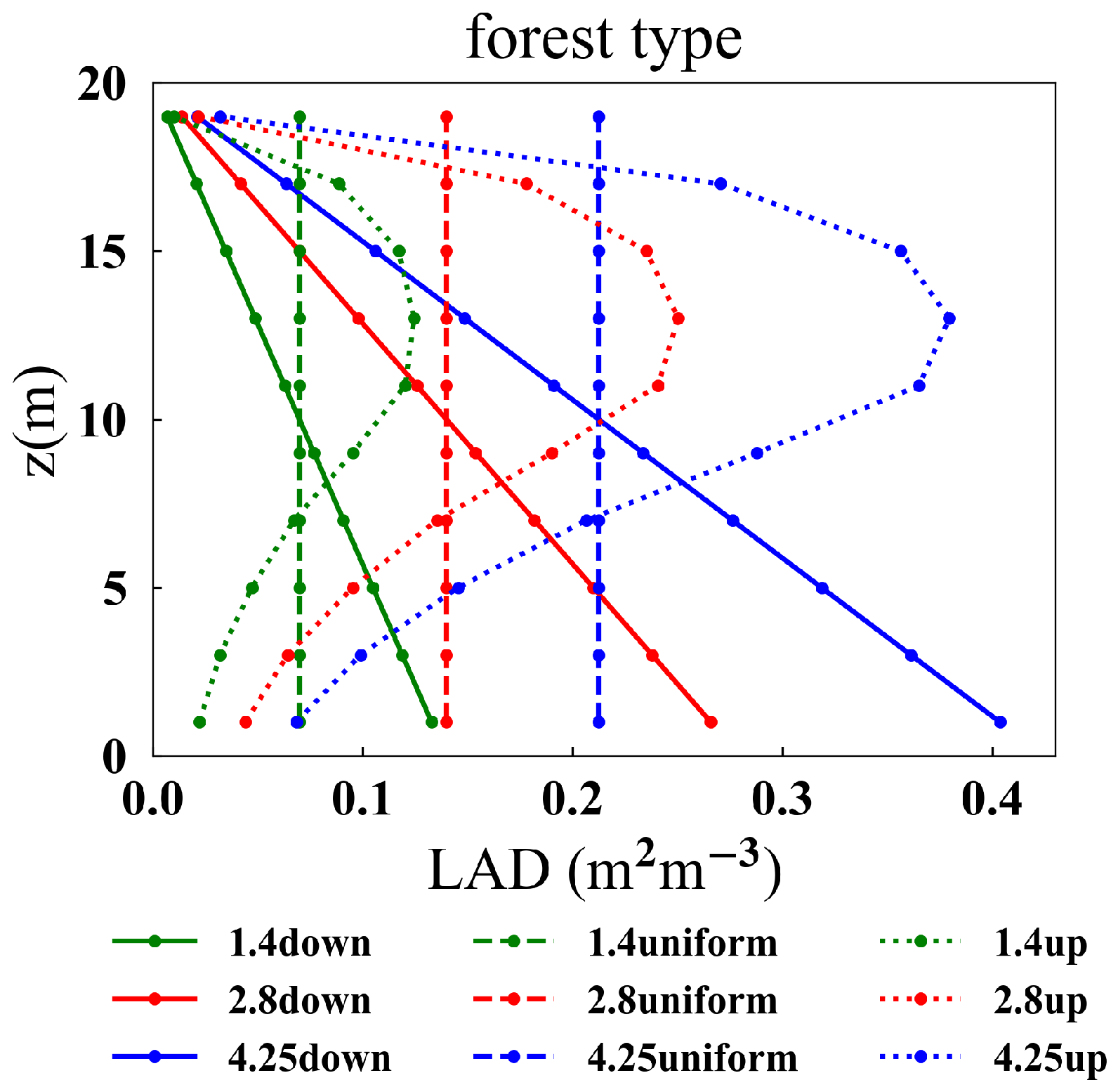
2.3. Forest Canopy Model

The aerodynamic drag by canopy elements was modeled using the porous body assumption. Specifically, the forest drag force ($f_i^f$) in Equation (2) was computed as

$$f_i^f=-C_d\alpha \left(z\right)\left|U\right|u_i,$$

(6)

where $C_d$ is the drag coefficient, $a\left(z\right)$ [$1/m$] is the LAD profile, U is the mean wind speed, and $u_i$ is the velocity component in the ith direction. In this work, $C_d$ is set to 0.15 according to refs. [53,54].

3. Computational Details and Test Case

3.1. Case Setup

The simulations were conducted in a rectangular computational domain, as shown in Figure 2. The domain size is $L_x\times L_y\times L_z=16D\times 8D\times 4D$ with the corresponding grid number $N_x\times N_y\times N_z=193\times 97\times 136$, where $x,y$, and z denote the streamwise, spanwise and vertical directions, respectively. The size of $L_y$ is twice as large as $L_z$ according to ref. [55]. Such a computational domain is widely used in the study of wind resources in forest terrain [56,57]. The wind turbine simulated has a hub height of 100 m, a rotor diameter of 100 m, and a thrust coefficient of $0.68$. The turbine model was placed at $(x,y)=(0,0)$. As in the experiments, a canopy height of $h=20$ m was used in the simulation. In the horizontal directions, the grid nodes were uniformly distributed $\mathsf{\Delta }x=\mathsf{\Delta }y\approx D/12$. In the vertical direction, 10 grid cells were used to discretize the canopy with a constant grid spacing of $\mathsf{\Delta }z=2$ m. The grid spacing was gradually stretched to $\mathsf{\Delta }z=2.5$ m from $z=20$ m to 50 m, and kept constant until $z=2D$. For $z>2D$, the grid was gradually stretched until the top boundary. Appendix A shows the grid dependency study for testing the employed grid resolution, showing converged results for the far wake characteristics, including both the time-averaged ones and the wake meandering statistics. As for the grid resolution required for the canopy flow, similar grid resolution was employed in the literature [29], which is enough to resolve the vertical variation in the canopy layer. The free-slip boundary condition was applied at the top boundary. At the bottom, the logarithmic law for rough walls was applied, using a roughness length $z_0=0.4$ m according to ref. [58]. The periodic boundary condition was applied in the transverse direction, being consistent with the precursory simulations.

The leaf area parameters were employed in the canopy model to mimic different forest types. For each forest canopy setup, two types of simulations with and without the wind turbine were conducted to provide a reference for the background turbulent boundary layer flow. The two simulations were performed with exactly the same settings, including the same boundaries, initial conditions, and time steps to produce synchronized results for analyses of instantaneous flow fields.

In order to examine the influence of the forest canopy on the wake characteristics of wind turbines, a set of canopy parameters was employed, consisting of three different vertical distributions of the LAD profile with three different values of LAI, which is defined as

$$\mathrm{LAI}={\int }_0^h\alpha \left(z\right)dz,$$

(7)

where $h=20$ m is the canopy height and $\alpha \left(z\right)$ is the vertical LAD profile data. The three distributions of the LAD profiles are shown in Figure 3, which are similar with those employed by Ma et al. [59]. The considered LAI are $\mathrm{LAI}=4.25,2.8,$ and $1.4$ for the dense, sparse, and very sparse forest cases, respectively [32,57].

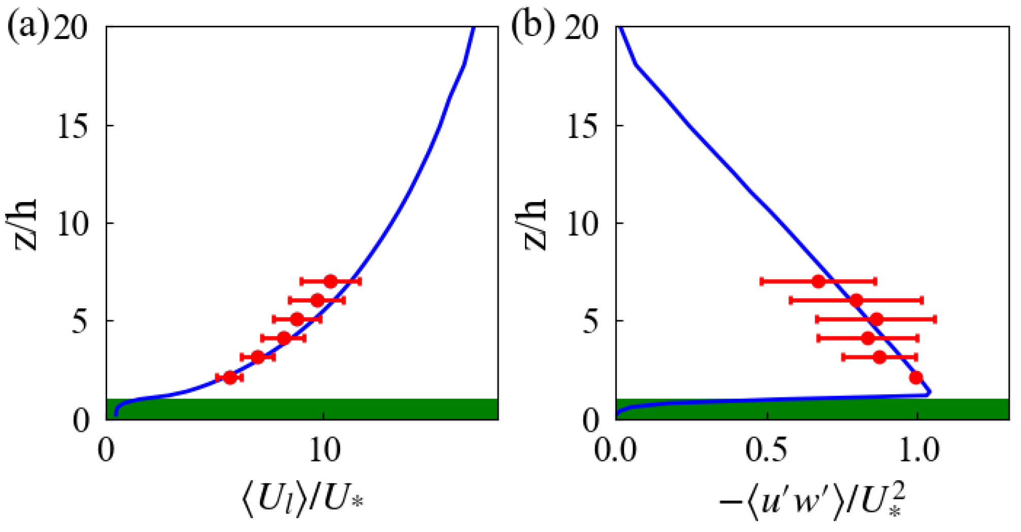
3.2. Validation of the Forest Canopy Model

In this subsection, we describe how the numerical approach was validated against field measurements. The measurements were taken at a test site at Ryningsnäs in southeastern Sweden, where the forest is predominantly Scots pine trees [60,61] and whose LAD is close to the 4.25up profile shown in Figure 3. Figure 4 compares the simulation results obtained by our numerical approach with the measurement for the normalized mean wind speed ($\langle U_l\rangle /U_{*}$) and the primary Reynolds shear stress ($-\langle u^{\prime }{w}^{\prime }\rangle /U_{*}^2$) in the streamwise direction. In this figure, the horizontal wind speed ($\langle U_l\rangle =\sqrt{{\langle u\rangle }^2+\langle v^2\rangle }$) and the primary Reynolds shear stress are normalized with the friction velocity ($U_{*}={[{\langle u^{\prime }{w}^{\prime }\rangle }_l^2+{\langle v^{\prime }{w}^{\prime }\rangle }_l^2]}^{1/4}$) evaluated at $z=2h$ [62]. A good agreement is observed between the simulation results and the measurements.

3.3. Inflows

In Figure 5, the inflows obtained from the precursory simulation are plotted. The relative difference in TKE (turbulence kinetic energy) among different LADs is larger than the difference in time-averaged velocity, with the maximum difference reaching approximately 30%. For the same LAI value, the TKE intensity is lowest for the “down” LAD profile and highest for the “uniform” LAD profile. Among the “uniform” LAD profiles with different LAI values, the TKE is largest for the case with an LAI of 2.8. Conversely, the effect of LAI on TKE is not significant for the “down” and “up” LAD profiles.

4. Results and Discussion

4.1. Scots Pine Tree (4.25up) Case and Flat Case

To examine the effect of the forest canopy on wake characteristics, the results from the 4.25up (Scots pine tree) and flat cases were compared.

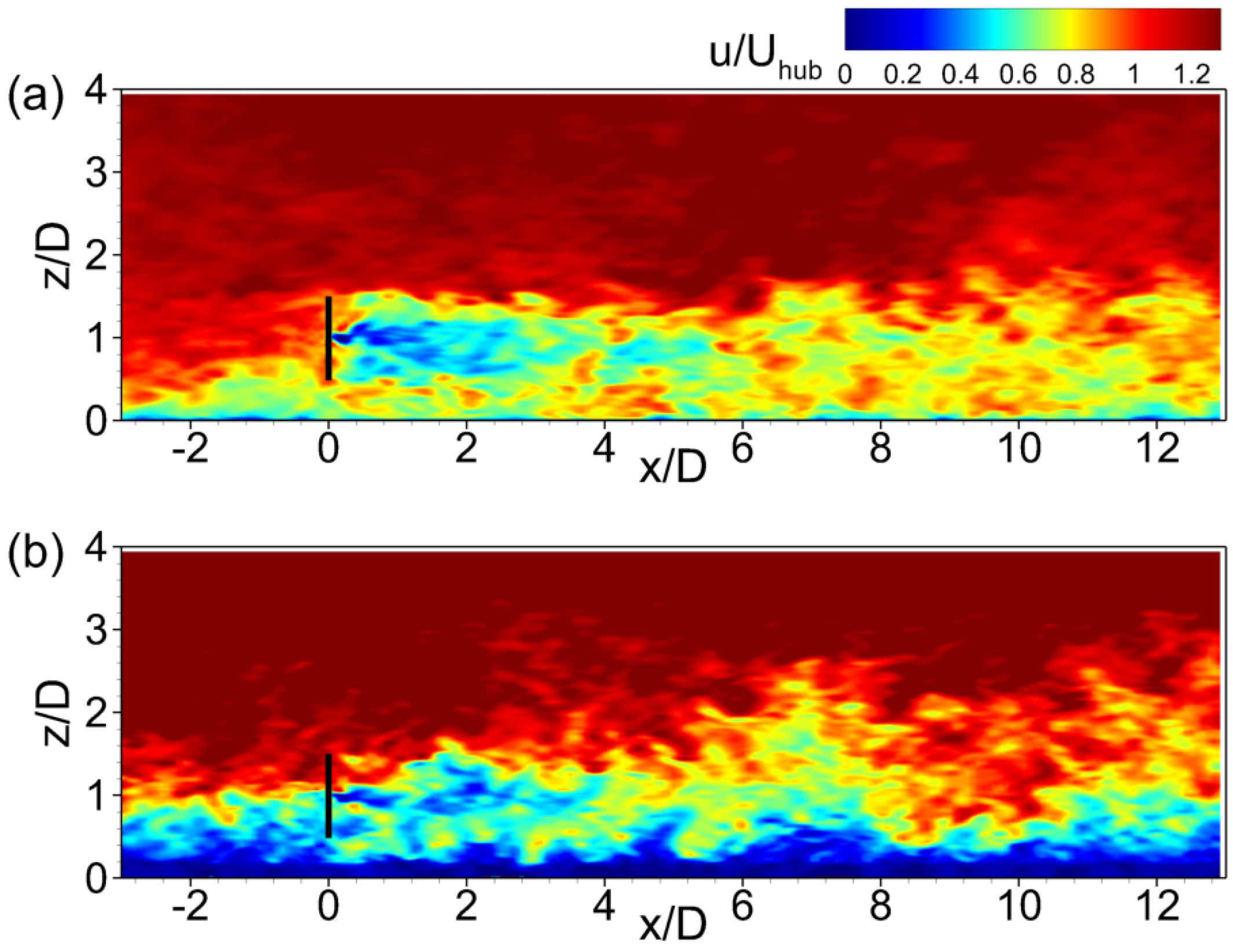
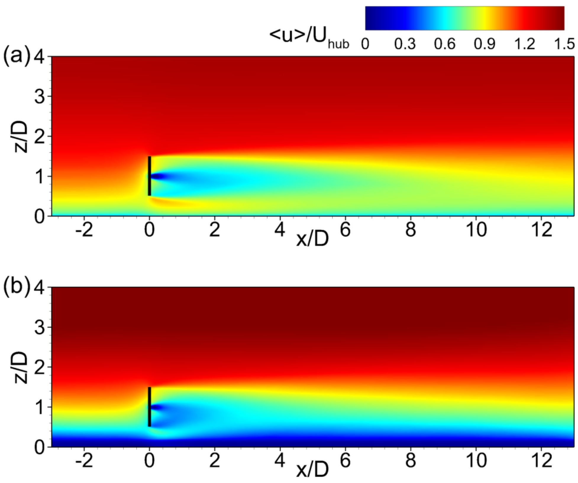
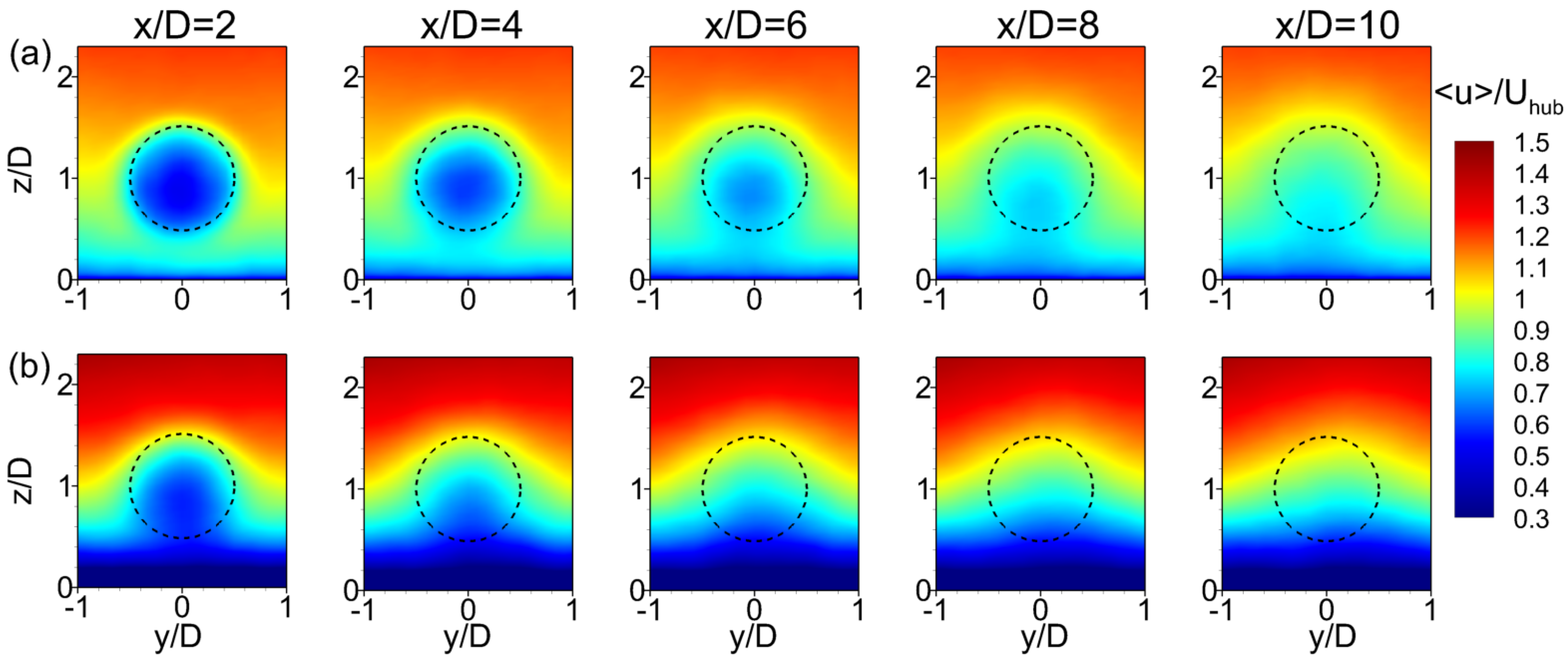
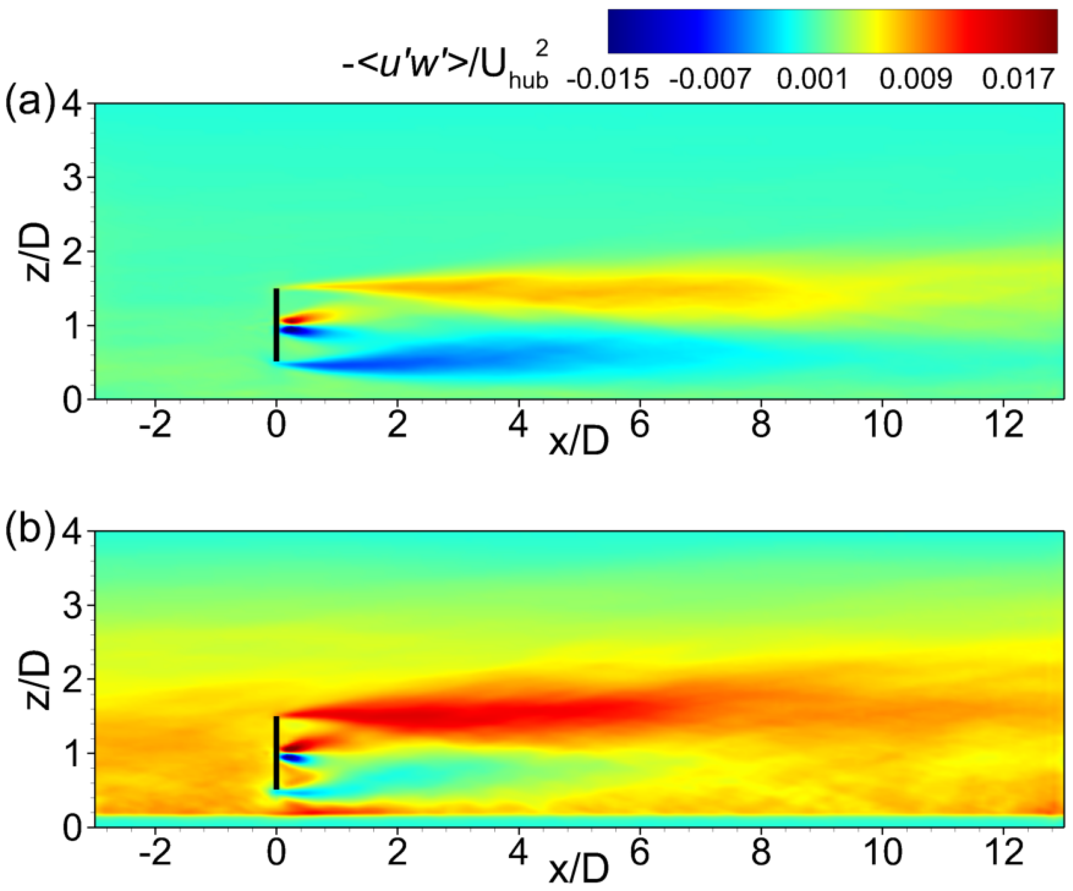
4.1.1. Instantaneous and Time-Averaged Wake Characteristics

We examined the contours of the instantaneous streamwise velocity from the two cases in Figure 6. The wake remained almost straight until about $2D$ downstream for the flat case, while it became unstable immediately downstream for the 4.25up case, with more energetic turbulent inflow. At further downstream locations, the wake of the wind turbine could hardly be distinguished from the background flow for the 4.25up case, showing a stronger interaction between the wake and the boundary layer, and a faster wake recovery compared to the flat case.

Figure 7 and Figure 8 display the time-averaged streamwise velocity contours in the x–z plane through the center of the rotor and the y–z plane located at different turbine downstream locations, i.e., $x/D$ = 2, 4, 6, 8, and 10. The time-averaged velocity field from the flat case and the 4.25up case were significantly different. Asymmetric distribution of the streamwise velocity component was observed in the far wake region due to the shear in the vertical direction.

The contours of turbulence kinetic energy ($k=\left(\langle {u^{\prime }}^2+{v^{\prime }}^2+{w^{\prime }}^2\rangle \right)/\left(2U_{hub}^2\right)$) were plotted in Figure 9 and Figure 10. As observed, both cases have a high TKE region in the top shear layer. Furthermore, the magnitude of the TKE decreases with downstream distance in both cases. However, the two cases show the difference in the peak turbulence intensity in terms of both the magnitude and the location. For the 4.25up case, the TKE is spread to a larger region with peak values around $2D$–$4D$ downstream of the turbine. In contrast, the case with flat terrain has a TKE peak further downstream ($4D$–$6D$). Another interesting observation in the 4.25up case is that the TKE in the lower part of the wake ($z<z_h$) is reduced when compared with the inflow, indicating a part of the TKE is extracted by the wind turbine.

To further reveal the influence of the forest canopy on the wake evolution, the primary Reynolds shear stress ($-\langle u^{\prime }{w}^{\prime }\rangle /U_{hub}^2$) contours were plotted in Figure 11 and Figure 12 to give insight into the momentum entrainment around the wake boundary. The maximum magnitude of Reynolds shear stress ($-\langle u^{\prime }{w}^{\prime }\rangle /U_{hub}^2$) is located in the range of $2D$–$4D$ for the 4.25up case and in the range of $4D$–$6D$ for the flat case. The magnitude of the Reynolds shear stress ($-\langle u^{\prime }{w}^{\prime }\rangle /U_{hub}^2$) is greater near the upper boundary of the wake for the 4.25up case when compared to the flat case, indicating a higher intensity of momentum mixing. Around the bottom boundary of the wake, on the other hand, the magnitude of the Reynolds shear stress ($-\langle u^{\prime }{w}^{\prime }\rangle /U_{hub}^2$) from the 4.25up case is smaller when compared to the flat case.

4.1.2. Mean Kinetic Energy Budget

To further understand the difference between the evolution of the turbine wakes in the 4.25up case and the flat case, different terms in the mean kinetic energy (MKE) budget equation were analyzed, which can be formulated as follows:

$$\begin{array}{cc}\hfill \frac{\partial 〈u_i〉〈u_i〉/2}{\partial t}=-〈u_j〉& \frac{\partial 〈u_i〉〈u_i〉/2}{\partial x_j}-\frac{\partial }{\partial x_j}\left(\frac{1}{\rho }\langle p\rangle 〈u_j〉+〈u_i^{\prime }{u}_j^{\prime }〉〈u_i〉-2\left(v+v_t\right)S_{ij}〈u_i〉\right)\hfill \\ \hfill & +〈u_i^{\prime }{u}_j^{\prime }〉\frac{\partial 〈u_i〉}{\partial x_j}-2\left(v+v_t\right)S_{ij}\frac{\partial 〈u_i〉}{\partial x_j}.\hfill \end{array}$$

(8)

Since the focus is on the time-averaged MKE, the time derivative term on the left-hand side was set to zero. The various terms on the right-hand side of the above equation are: (1) the mean convection; (2) the diffusion, which consists of the transport due to mean pressure, Reynolds stresses, and molecular and eddy viscosity; (3) the turbulence production, which represents the conversion of MKE to TKE; and (4) the dissipation.

We performed a surface integration on the y–z plane, to analyze how these terms would affect the recovery of MKE at different turbine downstream locations. The integral surface extends from $y_1=y_c-R$ to $y_2=y_c+R$ and $z_1=z_c-R$ to $z_2=z_c+R$ in the spanwise and vertical directions, respectively, with $y_c$ and $z_c$ being the turbine hub center location and $R=D/2$. All the terms are normalized by ${\displaystyle \frac{1}{2}D{U}_{hub}^3}$. The obtained integrated MKE equation is given as follows:

$$0=MC+PT+TC+DF+TP+DP,$$

(9)

where $MC$, $PT$, $TC$, $TP$, $DF$ and $DP$ denote the mean convection, pressure transport, turbulence convection, turbulence production, diffusion, and dissipation terms, respectively, which are computed as follows:

$$\begin{array}{cc}\hfill MC=& -{\int }_{y_1}^{y_2}{\int }_{z_1}^{z_2}〈u_j〉\frac{\partial \left(〈u_i〉〈u_i〉/2\right)}{\partial x_j}dzdy,\hfill \end{array}$$

(10)

$$\begin{array}{cc}\hfill PT=& -{\int }_{y_1}^{y_2}{\int }_{z_1}^{z_2}\frac{\partial \left(\langle p\rangle 〈u_j〉/\rho \right)}{\partial x_j}dzdy,\hfill \end{array}$$

(11)

$$\begin{array}{cc}\hfill TC=& -{\int }_{y_1}^{y_2}{\int }_{z_1}^{z_2}\frac{\partial \left(〈u_i^{\prime }{u}_j^{\prime }〉〈u_i〉\right)}{\partial x_j}dzdy,\hfill \end{array}$$

(12)

$$\begin{array}{cc}\hfill DF=& 2{\int }_{y_1}^{y_2}{\int }_{z_1}^{z_2}\frac{\partial \left(v+v_t\right)S_{ij}〈u_i〉}{\partial x_j}dzdy,\hfill \end{array}$$

(13)

$$\begin{array}{cc}\hfill TP=& {\int }_{y_1}^{y_2}{\int }_{z_1}^{z_2}〈u_i^{\prime }{u}_j^{\prime }〉\frac{\partial 〈u_i〉}{\partial x_j}dzdy,\hfill \end{array}$$

(14)

$$\begin{array}{cc}\hfill DP=& -2{\int }_{y_1}^{y_2}{\int }_{z_1}^{z_2}\left(v+v_t\right)S_{ij}\frac{\partial 〈u_i〉}{\partial x_j}dzdy.\hfill \end{array}$$

(15)

Figure 13 shows different terms in Equation (9) for the flat case (a) and the 4.25up case (b). It should be noted that, due to the high Reynolds number, the DF and DP terms are fairly small compared to the other terms, so these two terms can be ignored. A common feature observed in both cases is that the mean convection term is balanced with the pressure transport term in the near-wake region, showing that the kinetic energy gained from the convection is mainly consumed to recover the pressure. In the far-wake region, the mean convection (MC) term is mainly balanced with the turbulence convection (TC) term for the flat case. In contrast, in the 4.25up case, the turbulence convection (TC) term is mainly balanced with the sum of the mean convection (MC) term and the turbulence production (TP) term. The turbulence production (TP) term does not reduce to 0 as in the flat case because of the forest canopy but remains as a negative value, which transfers the energy from the mean flow to turbulence. This is also observed in the results in refs. [63,64]. Another notable difference is the turbulence convection (TC) term. The TC term in the 4.25up case has a clear peak compared to the flat case, and the peak magnitude of the TC term in the 4.25up case is higher than that in the flat case. Additionally, the peak position ($x/D\approx 0.5$) is closer to the wind turbine than the flat case ($x/D\approx 3$). Meanwhile, for the 4.25up case, the location where the MC term changes from positive to negative ($x/D\approx 1D$) is closer to the wind turbine than in the flat case due to the enhanced turbulence intensity of the background flow field in the presence of the forest canopy. A greater turbulence intensity is observed above the forest canopy, so the peak absolute values of the TP and TC terms are larger and located closer to the wind turbine. The above results suggest that the presence of the forest canopy leads to an increase in turbulence intensity, which enhances turbulence convection intensity and eventually speeds up the wake recovery.

Figure 14 shows the contours of the turbulence production term (−TP in Equation (9)) in the x–z plane for the flat case (left) and the 4.25up case (right). The TP term is significantly larger around the top tip when compared with that around the bottom tip and is distributed in a wider region for the 4.25up case. It is interesting to note that the magnitude of the TP term in the lower half of the wake is significantly smaller than that in the inflow for the 4.25up case, explaining the reason for the reduced TKE shown in Figure 9.

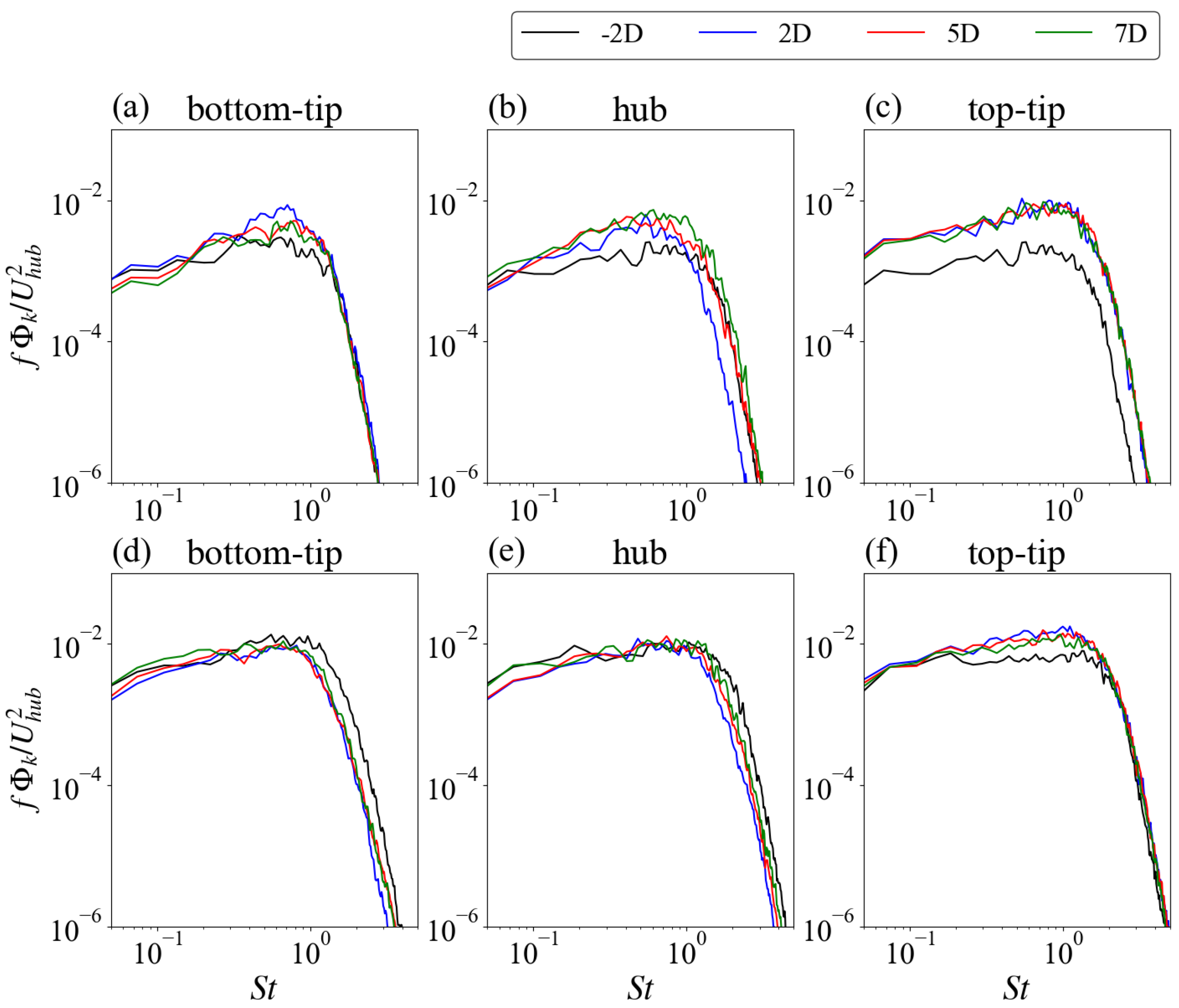
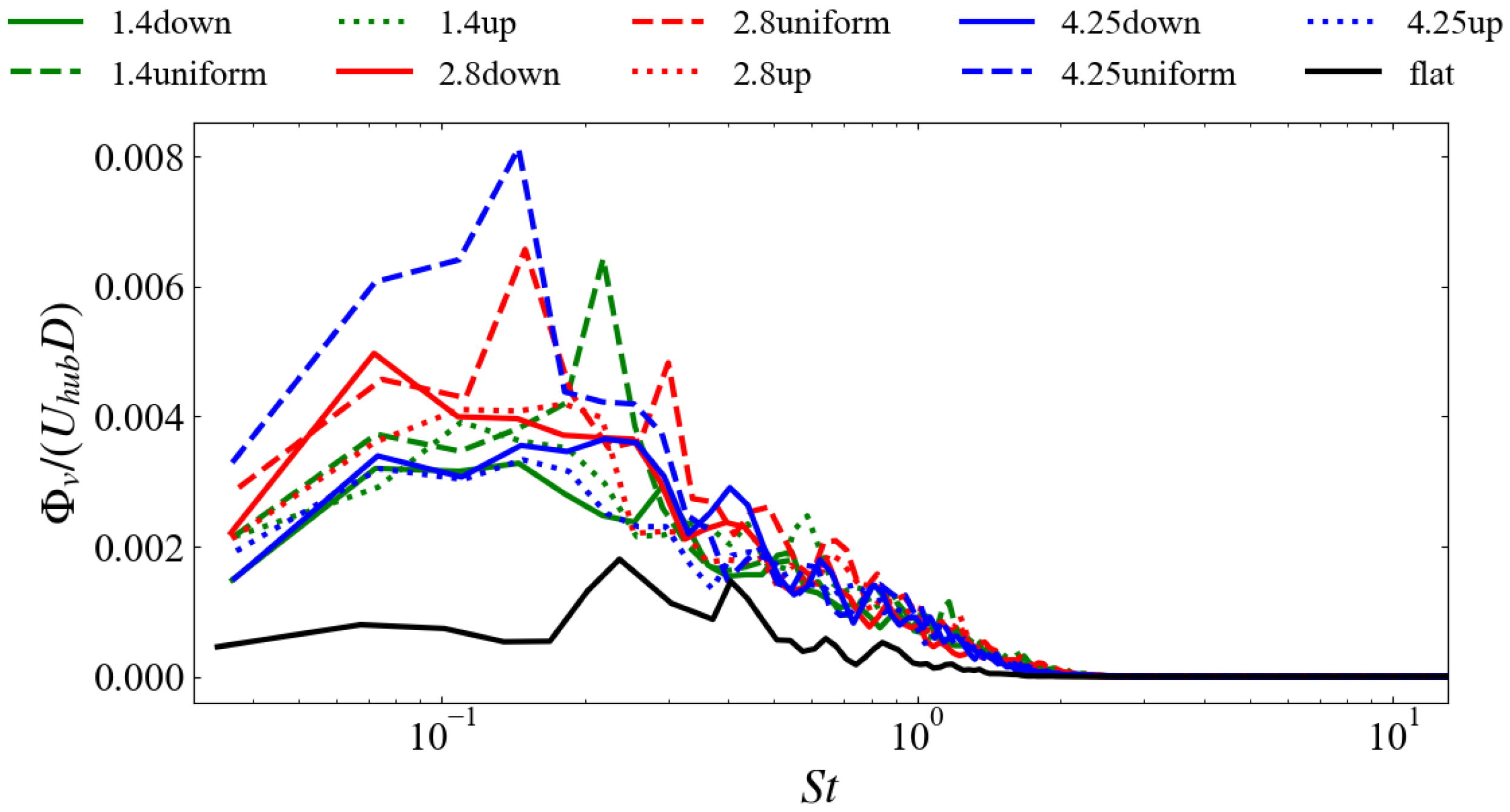
4.1.3. Power Spectral Density

The pre-multiplied power spectral density (PSD) of TKE was computed to examine the streamwise variation of TKE in the frequency space. The pre-multiplied PSD of TKE was computed via $f{\varphi }_k$ ($f{\varphi }_k=f({\varphi }_u+{\varphi }_v+{\varphi }_w)$, where ${\varphi }_u$, ${\varphi }_v$, and ${\varphi }_w$ are the PSDs of velocity fluctuations. The pre-multiplied PSDs of TKE at three different vertical locations (bottom tip, hub, and top tip) were examined in Figure 15 at various streamwise locations $x/D=\{-2,2,5,7\}$ for the flat case ((a)(b)(c)) and the 4.25up case ((d)(e)(f)).

From the results, we found that most of the TKE (i.e., the area enclosed by the pre-multiplied PSD) was concentrated in the range of $0.05<St<2.0$, being consistent with the experiments [65], numerical simulations [66], and theoretical analysis in refs. [67,68,69]. The intensities of TKE from the 4.25up case were, in general, higher than those from the flat case for all the frequencies for the same vertical location. The streamwise variations of the pre-multiplied PSDs were different at different vertical locations. At the top tip location, the intensities of TKE at all the frequencies increased due to the wind turbine wake for the flat case. For the 4.25up case, on the other hand, the increases in the intensities of TKE were only observed in the range of $St\in (0.2,2)$. At the hub height, the intensity of TKE increased significantly for $St<1$ for all the considered turbine downwind locations, while it decreased for $St>1$ at $x=2D$ turbine downwind for the flat case. For the 4.25up case, the intensities of TKE at the bottom tip and hub height locations were reduced for $St>1$ for all the considered turbine downwind locations.

4.2. Impacts of Different Forest Canopies

We examined the velocity deficits ($\mathsf{\Delta }U/U_{hub}$), wake-added TKE ($\mathsf{\Delta }k/U_{hub}^2$), and wake-added primary Reynolds shear stress ($\mathsf{\Delta }\langle u^{\prime }{w}^{\prime }\rangle /U_{hub}^2$) for the simulated cases with different types of forest canopies, which are defined as the difference between the two cases with and without a wind turbine as follows:

$$\mathsf{\Delta }U=\frac{U_{NT}-U}{U_{hub}},$$

(16)

$$\mathsf{\Delta }k=\frac{k-k_{NT}}{U_{hub}^2},$$

(17)

and

$$\mathsf{\Delta }\langle u^{\prime }{w}^{\prime }\rangle =\frac{\langle u^{\prime }{w}^{\prime }\rangle -\langle {u^{\prime }{w}^{\prime }\rangle }_{NT}}{U_{hub}^2},$$

(18)

respectively. The subscript ${·}_{NT}$ indicates the results from the simulations without a turbine.

4.2.1. Different Forest Densities

This subsection probes into the impact of LAIs on wind turbine wakes. Figure 16 shows the velocity deficit profiles. The recovery rate was the slowest when LAI = 1.4 and increased when increasing LAI from 1.4 to 2.8 or 4.25. The increasing trend, however, was different for different LAD distributions. The increase happened when increasing LAI from 1.4 to 2.8 for the down dense case shown in Figure 16a and from 2.8 to 4.25 for the uniform case shown in Figure 16b. For the top dense case shown in Figure 16c, on the other hand, the recovery rates were nearly the same for the three LAIs. For both the down dense and uniform cases, differences were observed at locations around the bottom tip, while they were barely noticed in the upper part of the wake.

The wake-added TKE is examined in Figure 17 for different LAIs. As shown in previous sections, the increase in TKE and the decrease in TKE were observed above and below the hub height, respectively. The same trend with LAI was not observed for different vertical distributions of LAD. For the down dense case shown in Figure 17a, the vertical range influenced by the wake was wider for $\mathrm{LAI}=2.8$. For the uniform dense and up dense cases shown in Figure 17b,c, the decrease in TKE was of the lowest magnitude for $\mathrm{LAI}=4.25$ at certain turbine downwind locations.

The wake-added primary Reynolds shear stresses ($\mathsf{\Delta }{u}^{\prime }{w}^{\prime }/U_{hub}^2$) are shown in Figure 18. The impact of LAI is small and all profiles nearly collapse together, which is different from that observed for the wake-added velocity deficit and wake-added TKE.

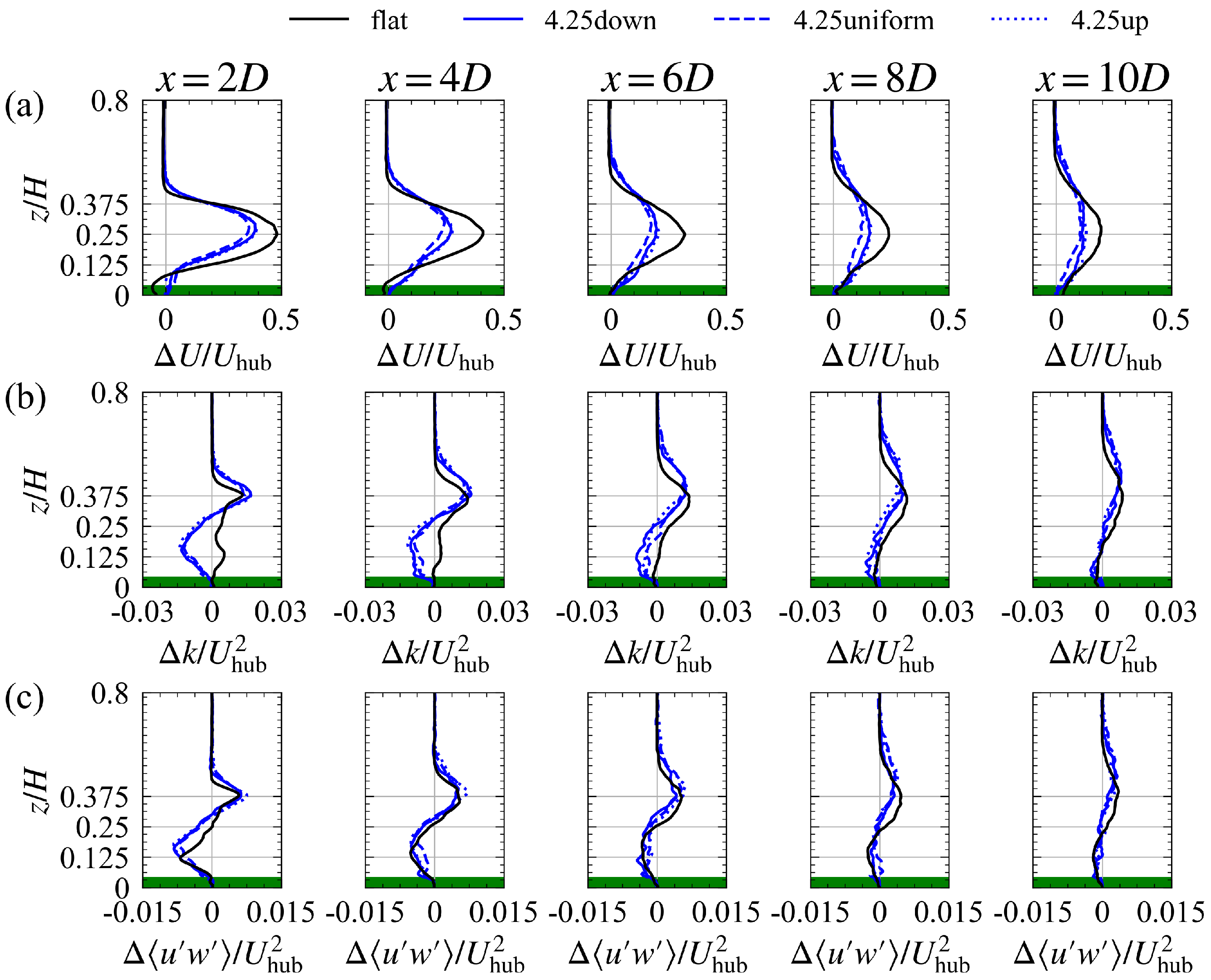
4.2.2. Different LAD Distributions

This subsection describes the impact of the LAD distribution on the wind turbine wake for the same LAI.

Figure 19 shows the velocity deficit, wake-added TKE ($\mathsf{\Delta }k/U_{hub}^2$), and wake-added primary Reynolds shear stress ($\mathsf{\Delta }{u}^{\prime }{w}^{\prime }/U_{hub}^2$) for the cases with $\mathrm{LAI}=4.25$. The wake recovery rate of the uniform dense case was somewhat faster compared with the other two LAD distributions. The $\mathsf{\Delta }k/U_{hub}^2$ and $\mathsf{\Delta }{u}^{\prime }{w}^{\prime }/U_{hub}^2$ from cases with different LAD distributions, on the other hand, were close to each other.

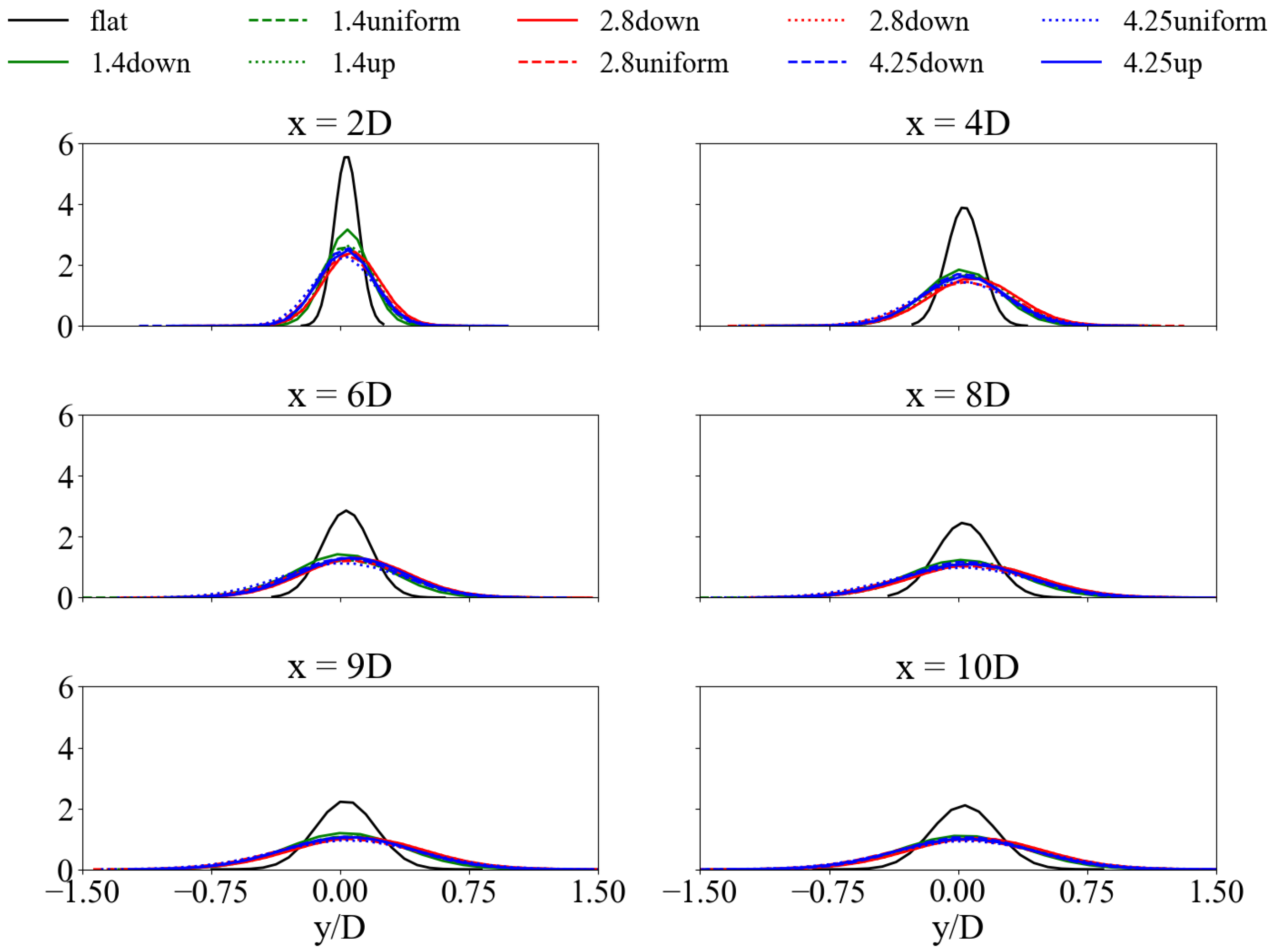
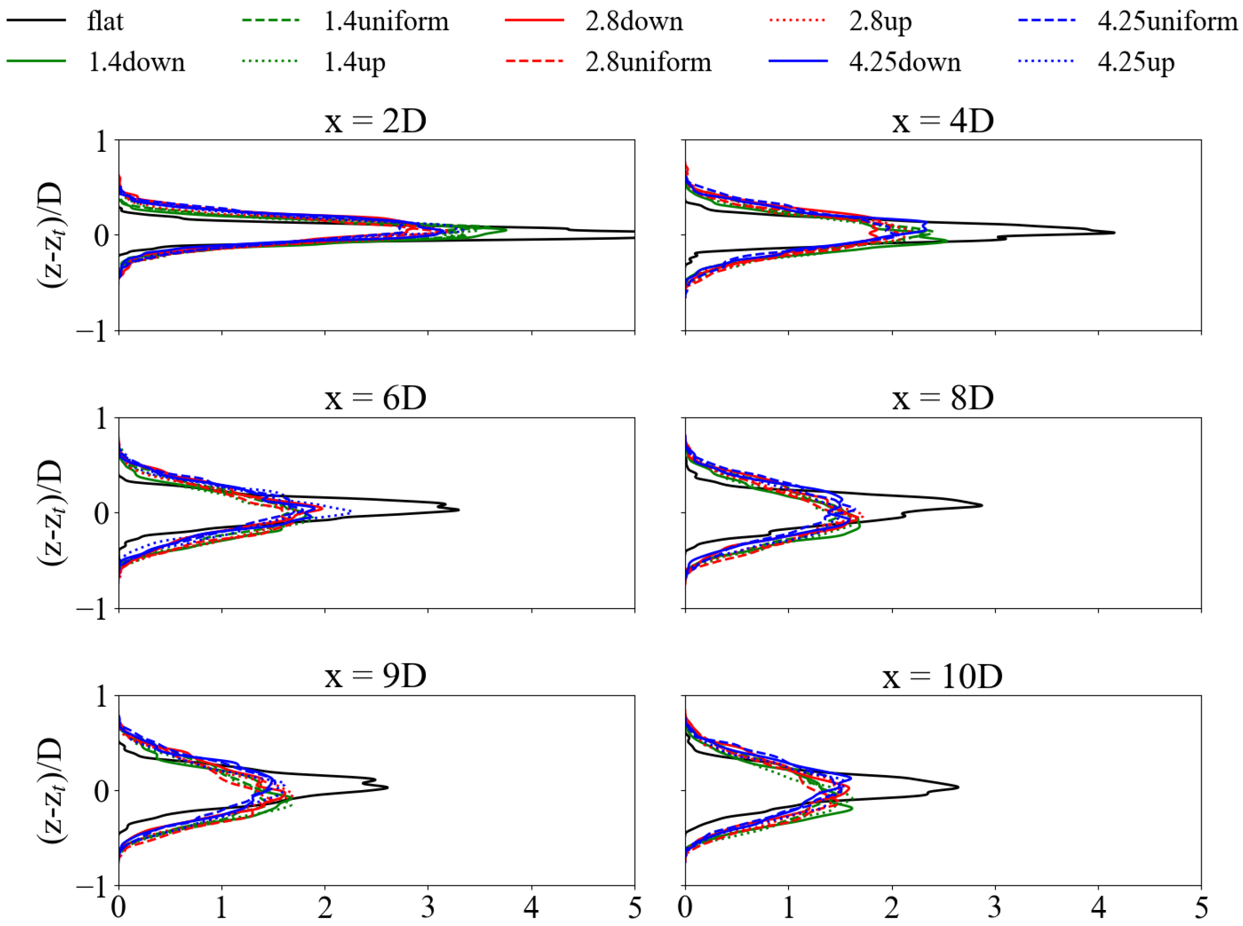
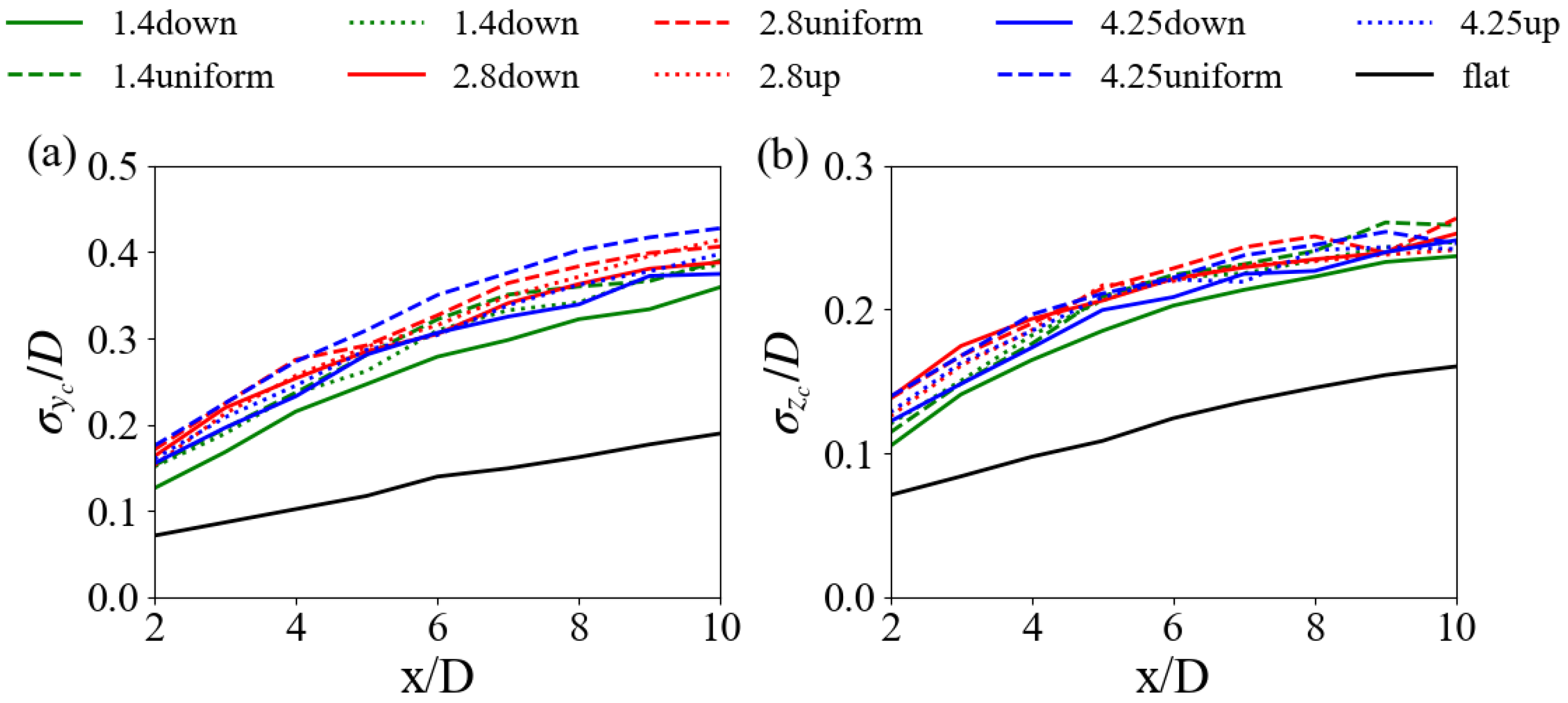
4.2.3. Wake Meandering Statistics

Wake meandering is a low-frequency, large-scale motion of wind turbine wakes, significantly impacting the power output and fatigue load of the downstream wind turbines [70,71,72]. In this section, the influence of different forest canopies on wake meandering characteristics is investigated and compared with the flat case.

The instantaneous wake position was calculated using the weighted average of the instantaneous streamwise velocity deficit [73] as follows:

$$y_c=\frac{\int {(u_{NT}-u)}^{2}ydy}{\int {(u_{NT}-u)}^{2}dy},$$

(19)

$$z_c=\frac{\int {(u_{NT}-u)}^{2}zdz}{\int {(u_{NT}-u)}^{2}dz},$$

(20)

where $y_c$ and $z_c$ are instantaneous wake centers in the spanwise and vertical directions, u is the instantaneous streamwise velocity, and $u_{NT}$ is the corresponding streamwise velocity from the simulation without a wind turbine at exactly the same turbine downstream location and time instant.

First, we show the probability density function (PDF) of the wake center positions at $x/D\in (2,4,6,8,9,10)$ for all cases in both spanwise ($y_c$) and vertical ($z_c$) directions. Figure 20 shows the PDF of $y_c$. As seen, the PDF resembles that of the Gaussian curve. As the wake travels downstream, the wake center is distributed in a wider range. Compared with the flat terrain, the forest canopy significantly increases the wake meandering amplitude. Figure 21 shows the PDF of $z_c$. At far away wake locations, the PDF of $z_c$ is somewhat skewed to the positions above the centerline, which is approximately symmetrical for the PDF of $y_c$. For PDFs of both $y_c$ and $z_c$, the differences between cases with different LADs are insignificant.

The downstream variations of the standard deviations of the wake center positions are examined in Figure 22. The forest canopy significantly enhances the wake meandering amplitude. The difference between different forest canopies is approximately $0.05D$. The meandering amplitude of the 1.4down case is the lowest among all the simulated cases.

The effect of the forest canopy on the dominant frequency of wake meandering is shown in Figure 23 by examining the PSD of the wake centerline spanwise velocity fluctuations at $x/D=5$. The dominant frequency of wake meandering is approximately $St\approx 0.25$ for the case with flat terrain, while it is around $St=0.1$∼0.15 with a higher amplitude for the cases with forest canopies. As for the effects of different canopies, the amplitude of PSD for $\mathrm{LAI}=1.4$ is in general lower than other cases. With the increase in the LAI value, a consistent trend is not observed. For the effects of vertical LAD distributions, the amplitude of PSD from the case with uniform LAD is in general higher when compared with other cases with the same LAI.

5. Conclusions

In this work, large-eddy simulation of wind turbine wakes in forest terrain was carried out. The influences of forests on the statistics of wind turbine wakes were systematically investigated for different vertical distributions of leaf area density (LAD) and different values of leaf area index (LAI).

The simulation results show that the wind turbine wake in the forest canopy is characterized by faster wake recovery and higher turbulence kinetic energy (TKE) when compared with those from the flat terrain. Analysis of the mean kinetic energy (MKE) budget equation shows that the accelerated wake recovery is mainly due to the enhanced turbulence convection in the forest terrain. One interesting phenomenon is that the TKE below the centerline from $1D$ to $8D$ turbine downstream is lower than that of the inflow for all the simulated forest canopies, which is observed only along the wake centerline for a short distance for the flat terrain. Further investigation into the power spectral density shows that such reduction in TKE exists mainly at higher frequencies with $St>1.0$. In the region along the top tip, the TKE is increased for both cases, which occurs for all the considered frequencies for the flat terrain and in the range of $St\in (0.2,2)$ for the forest terrain. Compared with the vertical distribution of LAD, the LAI affects the wind turbine wake in the forest terrain in a more significant way for the considered cases. For the same LAI, the wake-added TKE and Reynolds shear stresses collapse well with each other. Overall, the wake-added TKE from the forest cases is significantly different from the flat case, while the wake-added primary Reynolds shear stresses are close to each other. The amplitude of wake meandering is increased by approximately 2 times in the spanwise direction and 1.5 times in the vertical direction from those of the flat terrain. The differences in meandering magnitude are approximately $0.5D$ for the simulated cases. The dominant frequency of wake meandering is observed to be lower for the forest terrain case ($St\in (0.1,0.15)$) when compared with the flat case ($St\approx 0.25$).

This work focused on turbulence statistics and wake meandering. According to the results, some suggestions can be put forward for placing wind turbines in forest terrain. On one hand, it is necessary to pay attention to the impact of high TKE of the incoming flow on the increases in dynamic load and power fluctuations. On the other hand, wind turbines can be placed closely in the streamwise direction as a result of the observed faster wake recovery when compared with the flat terrain.

In this study, the forest was considered to be homogeneous in the horizontal direction. Only a stand-alone wind turbine was simulated. How a heterogeneous forest canopy interacts with wind turbine wakes, and what the effects of arrays of wind turbines on the wind field above and within the forest are need to be investigated in a future study. Moreover, studies on the interaction between the near wake vortex system (e.g., tip vortex and hub vortex) and the forest canopy are certainly important and should be carried out in the future using an actuator surface model and forest parameterization models of higher fidelity. As the wind turbine wake can significantly change the turbulence above the forest canopy, it certainly will affect the humidity and temperature in the forest, which is of great importance to our living environment and should be investigated systematically [74,75,76].

References

1. Holechek, J.L.; Geli, H.M.E.; Sawalhah, M.N.; Valdez, R. A Global Assessment: Can Renewable Energy Replace Fossil Fuels by 2050? Sustainability 2022, 14, 4792. [Google Scholar] [CrossRef]
2. Li, W.; Xu, S.; Qian, B.; Gao, X.; Zhu, X.; Shi, Z.; Liu, W.; Hu, Q. Large-Scale Wind Turbine’s Load Characteristics Excited by the Wind and Grid in Complex Terrain: A Review. Sustainability 2022, 14, 17051. [Google Scholar] [CrossRef]
3. Veers, P.; Dykes, K.; Lantz, E.; Barth, S.; Bottasso, C.L.; Carlson, O.; Clifton, A.; Green, J.; Green, P.; Holttinen, H.; et al. Grand challenges in the science of wind energy. Science 2019, 366, eaau2027. [Google Scholar] [CrossRef] [Green Version]
4. Meyers, J.; Bottasso, C.; Dykes, K.; Fleming, P.; Gebraad, P.; Giebel, G.; Göçmen, T.; Van Wingerden, J.W. Wind farm flow control: Prospects and challenges. Wind Energy Sci. 2022, 7, 2271–2306. [Google Scholar] [CrossRef]
5. De Cillis, G.; Cherubini, S.; Semeraro, O.; Leonardi, S.; De Palma, P. The influence of incoming turbulence on the dynamic modes of an NREL-5MW wind turbine wake. Renew. Energy 2022, 183, 601–616. [Google Scholar] [CrossRef]
6. Zhang, W.; Markfort, C.D.; Porté-Agel, F. Near-wake flow structure downwind of a wind turbine in a turbulent boundary layer. Exp. Fluids 2012, 52, 1219–1235. [Google Scholar] [CrossRef] [Green Version]
7. Stein, V.P.; Kaltenbach, H.J. Non-Equilibrium Scaling Applied to the Wake Evolution of a Model Scale Wind Turbine. Energies 2019, 12, 2763. [Google Scholar] [CrossRef] [Green Version]
8. Mendoza, V.; Chaudhari, A.; Goude, A. Performance and wake comparison of horizontal and vertical axis wind turbines under varying surface roughness conditions. Wind Energy 2019, 22, 458–472. [Google Scholar] [CrossRef]
9. Kethavath, N.N.; Mondal, K.; Ghaisas, N.S. Large-eddy simulation and analytical modeling study of the wake of a wind turbine behind an abrupt rough-to-smooth surface roughness transition. Phys. Fluids 2022, 34, 125117. [Google Scholar] [CrossRef]
10. Wu, Y.T.; Porté-Agel, F. Atmospheric turbulence effects on wind-turbine wakes: An LES study. Energies 2012, 5, 5340–5362. [Google Scholar] [CrossRef] [Green Version]
11. Yang, X.; Pakula, M.; Sotiropoulos, F. Large-eddy simulation of a utility-scale wind farm in complex terrain. Appl. Energy 2018, 229, 767–777. [Google Scholar] [CrossRef]
12. Tobin, N.; Chamorro, L.P. Modulation of turbulence scales passing through the rotor of a wind turbine. J. Turbul. 2019, 20, 21–31. [Google Scholar] [CrossRef]
13. Jin, Y.; Liu, H.; Aggarwal, R.; Singh, A.; Chamorro, L.P. Effects of freestream turbulence in a model wind turbine wake. Energies 2016, 9, 830. [Google Scholar] [CrossRef] [Green Version]
14. Churchfield, M.J.; Lee, S.; Michalakes, J.; Moriarty, P.J. A numerical study of the effects of atmospheric and wake turbulence on wind turbine dynamics. J. Turbul. 2012, 13, N14. [Google Scholar] [CrossRef]
15. Abkar, M.; Porté-Agel, F. Influence of atmospheric stability on wind-turbine wakes: A large-eddy simulation study. Phys. Fluids 2015, 27, 035104. [Google Scholar] [CrossRef] [Green Version]
16. Du, B.; Ge, M.; Zeng, C.; Cui, G.; Liu, Y. Influence of atmospheric stability on wind-turbine wakes with a certain hub-height turbulence intensity. Phys. Fluids 2021, 33, 055111. [Google Scholar] [CrossRef]
17. Ning, X.; Wan, D. LES Study of Wake Meandering in Different Atmospheric Stabilities and Its Effects on Wind Turbine Aerodynamics. Sustainability 2019, 11, 6939. [Google Scholar] [CrossRef] [Green Version]
18. Li, Z.; Yang, X. Large-eddy simulation on the similarity between wakes of wind turbines with different yaw angles. J. Fluid Mech. 2021, 921, A11. [Google Scholar] [CrossRef]
19. Li, Z.; Dong, G.; Yang, X. Onset of wake meandering for a floating offshore wind turbine under side-to-side motion. J. Fluid Mech. 2022, 934, A29. [Google Scholar] [CrossRef]
20. Yang, D.; Meneveau, C.; Shen, L. Effect of downwind swells on offshore wind energy harvesting—A large-eddy simulation study. Renew. Energy 2014, 70, 11–23. [Google Scholar] [CrossRef]
21. Stevens, R.J.; Martínez-Tossas, L.A.; Meneveau, C. Comparison of wind farm large eddy simulations using actuator disk and actuator line models with wind tunnel experiments. Renew. Energy 2018, 116, 470–478. [Google Scholar] [CrossRef]
22. Bastankhah, M.; Porté-Agel, F. Wind tunnel study of the wind turbine interaction with a boundary-layer flow: Upwind region, turbine performance, and wake region. Phys. Fluids 2017, 29, 065105. [Google Scholar] [CrossRef]
23. Lignarolo, L.; Ragni, D.; Krishnaswami, C.; Chen, Q.; Ferreira, C.S.; Van Bussel, G. Experimental analysis of the wake of a horizontal-axis wind-turbine model. Renew. Energy 2014, 70, 31–46. [Google Scholar] [CrossRef]
24. Abraham, A.; Hong, J. Characterization of atmospheric coherent structures and their impact on a utility-scale wind turbine. Flow 2022, 2, E5. [Google Scholar] [CrossRef]
25. Hong, J.; Toloui, M.; Chamorro, L.P.; Guala, M.; Howard, K.; Riley, S.; Tucker, J.; Sotiropoulos, F. Natural snowfall reveals large-scale flow structures in the wake of a 2.5-MW wind turbine. Nat. Commun. 2014, 5, 4216. [Google Scholar] [CrossRef] [Green Version]
26. Hong, J.; Abraham, A. Snow-powered research on utility-scale wind turbine flows. Acta Mech. Sin. 2020, 36, 339–355. [Google Scholar] [CrossRef] [Green Version]
27. Elgendi, M.; AlMallahi, M.; Abdelkhalig, A.; Selim, M.Y. A Review of Wind Turbines in Complex Terrain. Int. J. Thermofluids 2023, 17, 100289. [Google Scholar] [CrossRef]
28. Zendehbad, M.; Chokani, N.; Abhari, R.S. Impact of forested fetch on energy yield and maintenance of wind turbines. Renew. Energy 2016, 96, 548–558. [Google Scholar] [CrossRef]
29. Nebenführ, B.; Davidson, L. Prediction of wind-turbine fatigue loads in forest regions based on turbulent LES inflow fields. Wind Energy 2017, 20, 1003–1015. [Google Scholar] [CrossRef]
30. Agafonova, O.; Avramenko, A.; Chaudhari, A.; Hellsten, A. Effects of the canopy created velocity inflection in the wake development in a large wind turbine array. Proc. J. Phys. Conf. Ser. 2016, 753, 032001. [Google Scholar] [CrossRef]
31. Chougule, A.; Mann, J.; Segalini, A.; Dellwik, E. Spectral tensor parameters for wind turbine load modeling from forested and agricultural landscapes. Wind Energy 2015, 18, 469–481. [Google Scholar] [CrossRef] [Green Version]
32. Adedipe, T.A.; Chaudhari, A.; Kauranne, T. Impact of different forest densities on atmospheric boundary-layer development and wind-turbine wake. Wind Energy 2020, 23, 1165–1180. [Google Scholar] [CrossRef]
33. Cheng, S.; Elgendi, M.; Lu, F.; Chamorro, L.P. On the Wind Turbine Wake and Forest Terrain Interaction. Energies 2021, 14, 7204. [Google Scholar] [CrossRef]
34. Belcher, S.E.; Harman, I.N.; Finnigan, J.J. The wind in the willows: Flows in forest canopies in complex terrain. Annu. Rev. Fluid Mech. 2012, 44, 479–504. [Google Scholar] [CrossRef]
35. Matsfelt, J.; Davidson, L. Large eddy simulation: A study of clearings in forest and their effect on wind turbines. Wind Energy 2021, 24, 1388–1406. [Google Scholar] [CrossRef]
36. Porté-Agel, F.; Bastankhah, M.; Shamsoddin, S. Wind-turbine and wind-farm flows: A review. Bound. Layer Meteorol. 2020, 174, 1–59. [Google Scholar] [CrossRef] [PubMed] [Green Version]
37. Yang, X.; Sotiropoulos, F.; Conzemius, R.J.; Wachtler, J.N.; Strong, M.B. Large-eddy simulation of turbulent flow past wind turbines/farms: The Virtual Wind Simulator (VWiS). Wind Energy 2015, 18, 2025–2045. [Google Scholar] [CrossRef]
38. Yang, X.; Milliren, C.; Kistner, M.; Hogg, C.; Marr, J.; Shen, L.; Sotiropoulos, F. High-fidelity simulations and field measurements for characterizing wind fields in a utility-scale wind farm. Appl. Energy 2021, 281, 116115. [Google Scholar] [CrossRef]
39. Yang, X.; Sotiropoulos, F. A new class of actuator surface models for wind turbines. Wind Energy 2018, 21, 285–302. [Google Scholar] [CrossRef] [Green Version]
40. Germano, M.; Piomelli, U.; Moin, P.; Cabot, W.H. A dynamic subgrid-scale eddy viscosity model. Phys. Fluids A Fluid Dyn. 1991, 3, 1760–1765. [Google Scholar] [CrossRef] [Green Version]
41. Li, Z.; Yang, X. Evaluation of actuator disk model relative to actuator surface model for predicting utility-scale wind turbine wakes. Energies 2020, 13, 3574. [Google Scholar] [CrossRef]
42. Yang, X.; Khosronejad, A.; Sotiropoulos, F. Large-eddy simulation of a hydrokinetic turbine mounted on an erodible bed. Renew. Energy 2017, 113, 1419–1433. [Google Scholar] [CrossRef]
43. Foti, D.; Yang, X.; Campagnolo, F.; Maniaci, D.; Sotiropoulos, F. Wake meandering of a model wind turbine operating in two different regimes. Phys. Rev. Fluids 2018, 3, 054607. [Google Scholar] [CrossRef]
44. Kang, S.; Yang, X.; Sotiropoulos, F. On the onset of wake meandering for an axial flow turbine in a turbulent open channel flow. J. Fluid Mech. 2014, 744, 376–403. [Google Scholar] [CrossRef]
45. Foti, D.; Yang, X.; Guala, M.; Sotiropoulos, F. Wake meandering statistics of a model wind turbine: Insights gained by large eddy simulations. Phys. Rev. Fluids 2016, 1, 044407. [Google Scholar] [CrossRef]
46. Chawdhary, S.; Hill, C.; Yang, X.; Guala, M.; Corren, D.; Colby, J.; Sotiropoulos, F. Wake characteristics of a TriFrame of axial-flow hydrokinetic turbines. Renew. Energy 2017, 109, 332–345. [Google Scholar] [CrossRef] [Green Version]
47. Yang, X.; Sotiropoulos, F. LES investigation of infinite staggered wind-turbine arrays. Proc. J. Phys. Conf. Ser. 2014, 555, 012109. [Google Scholar] [CrossRef]
48. Dong, G.; Li, Z.; Qin, J.; Yang, X. How far the wake of a wind farm can persist for? Theor. Appl. Mech. Lett. 2022, 12, 100314. [Google Scholar] [CrossRef]
49. Yang, X.; Sotiropoulos, F. On the predictive capabilities of LES-actuator disk model in simulating turbulence past wind turbines and farms. In Proceedings of the 2013 American Control Conference, Washington, DC, USA, 17–19 June 2013; pp. 2878–2883. [Google Scholar]
50. Foti, D.; Yang, X.; Shen, L.; Sotiropoulos, F. Effect of wind turbine nacelle on turbine wake dynamics in large wind farms. J. Fluid Mech. 2019, 869, 1–26. [Google Scholar] [CrossRef]
51. Breton, S.P.; Sumner, J.; Sørensen, J.N.; Hansen, K.S.; Sarmast, S.; Ivanell, S. A survey of modelling methods for high-fidelity wind farm simulations using large eddy simulation. Philos. Trans. R. Soc. A Math. Phys. Eng. Sci. 2017, 375, 20160097. [Google Scholar] [CrossRef] [Green Version]
52. Li, Z.; Liu, X.; Yang, X. Review of Turbine Parameterization Models for Large-Eddy Simulation of Wind Turbine Wakes. Energies 2022, 15, 6533. [Google Scholar] [CrossRef]
53. Adedipe, T.; Chaudhari, A.; Hellsten, A.; Kauranne, T.; Haario, H. Numerical Investigation on the Effects of Forest Heterogeneity on Wind-Turbine Wake. Energies 2022, 15, 1896. [Google Scholar] [CrossRef]
54. Schröttle, J.; Piotrowski, Z.; Gerz, T.; Englberger, A.; Dörnbrack, A. Wind turbine wakes in forest and neutral plane wall boundary layer large-eddy simulations. Proc. J. Phys. Conf. Ser. 2016, 753, 032058. [Google Scholar] [CrossRef] [Green Version]
55. Mason, P.J.; Thomson, D. Large-eddy simulations of the neutral-static-stability planetary boundary layer. Q. J. R. Meteorol. Soc. 1987, 113, 413–443. [Google Scholar] [CrossRef]
56. Agafonova, O. A Numerical Study of Forest Influences on the Atmospheric Boundary Layer and Wind Turbines. Ph.D. Thesis, Lappeenranta University of Technology, Lappeenranta, Finland, 2017. [Google Scholar]
57. Nebenführ, B.; Davidson, L. Large-eddy simulation study of thermally stratified canopy flow. Bound. Layer Meteorol. 2015, 156, 253–276. [Google Scholar] [CrossRef] [Green Version]
58. Shaw, R.H.; Patton, E.G. Canopy element influences on resolved-and subgrid-scale energy within a large-eddy simulation. Agric. For. Meteorol. 2003, 115, 5–17. [Google Scholar] [CrossRef] [Green Version]
59. Ma, Y.; Liu, H.; Banerjee, T.; Katul, G.G.; Yi, C.; Pardyjak, E.R. The effects of canopy morphology on flow over a two-dimensional isolated ridge. J. Geophys. Res. Atmos. 2020, 125, e2020JD033027. [Google Scholar] [CrossRef]
60. Mohr, M.; Arnqvist, J.; Abedi, H.; Alfredsson, H.; Baltscheffsky, M.; Bergström, H.; Carlén, I.; Davidson, L.; Segalini, A.; Söderberg, S. Wind Power in Forests II: Forest Wind; Energiforsk: Stockholm, Sweden, 2018. [Google Scholar]
61. Abedi, H.; Sarkar, S.; Johansson, H. Numerical modelling of neutral atmospheric boundary layer flow through heterogeneous forest canopies in complex terrain (a case study of a Swedish wind farm). Renew. Energy 2021, 180, 806–828. [Google Scholar] [CrossRef]
62. Shao, X.; Santasmasas, M.C.; Xue, X.; Niu, J.; Davidson, L.; Revell, A.J.; Yao, H.D. Near-wall modeling of forests for atmosphere boundary layers using lattice Boltzmann method on GPU. Eng. Appl. Comput. Fluid Mech. 2022, 16, 2142–2155. [Google Scholar] [CrossRef]
63. Yue, W.; Meneveau, C.; Parlange, M.B.; Zhu, W.; Kang, H.S.; Katz, J. Turbulent kinetic energy budgets in a model canopy: Comparisons between LES and wind-tunnel experiments. Environ. Fluid Mech. 2008, 8, 73–95. [Google Scholar] [CrossRef] [Green Version]
64. Chen, B.; Chamecki, M. Turbulent kinetic energy budgets over gentle topography covered by forests. J. Atmos. Sci. 2023, 80, 91–109. [Google Scholar] [CrossRef]
65. Turner V, J.J.; Wosnik, M. Wake meandering in a model wind turbine array in a high Reynolds number turbulent boundary layer. Proc. J. Phys. Conf. Ser. 2020, 1452, 012073. [Google Scholar] [CrossRef]
66. Foti, D.; Yang, X.; Sotiropoulos, F. Similarity of wake meandering for different wind turbine designs for different scales. J. Fluid Mech. 2018, 842, 5–25. [Google Scholar] [CrossRef]
67. Mao, X.; Sørensen, J. Far-wake meandering induced by atmospheric eddies in flow past a wind turbine. J. Fluid Mech. 2018, 846, 190–209. [Google Scholar] [CrossRef] [Green Version]
68. Gupta, V.; Wan, M. Low-order modelling of wake meandering behind turbines. J. Fluid Mech. 2019, 877, 534–560. [Google Scholar] [CrossRef] [Green Version]
69. Sarmast, S.; Dadfar, R.; Mikkelsen, R.F.; Schlatter, P.; Ivanell, S.; Sørensen, J.N.; Henningson, D.S. Mutual inductance instability of the tip vortices behind a wind turbine. J. Fluid Mech. 2014, 755, 705–731. [Google Scholar] [CrossRef] [Green Version]
70. Larsen, G.C.; Aagaard Madsen, H.; Bingöl, F. Dynamic Wake Meandering Modeling; Risoe National Lab., DTU: Roskilde, Denmark, 2007. [Google Scholar]
71. Rinker, J.M.; Soto Sagredo, E.; Bergami, L. The Importance of wake meandering on wind turbine fatigue loads in wake. Energies 2021, 14, 7313. [Google Scholar] [CrossRef]
72. Yang, X.; Sotiropoulos, F. A Review on the Meandering of Wind Turbine Wakes. Energies 2019, 12, 4725. [Google Scholar] [CrossRef] [Green Version]
73. Bastankhah, M. Interaction of Atmospheric Boundary Layer Flow with Wind Turbines; Technical Report; EPFL: Lausanne, Switzerland, 2017. [Google Scholar]
74. Thess, A.D.; Lengsfeld, P. Side Effects of Wind Energy: Review of Three Topics—Status and Open Questions. Sustainability 2022, 14, 16186. [Google Scholar] [CrossRef]
75. Colafranceschi, D.; Sala, P.; Manfredi, F. Nature of the wind, the culture of the landscape: Toward an energy sustainability project in Catalonia. Sustainability 2021, 13, 7110. [Google Scholar] [CrossRef]
76. van der Waal, E.C.; van der Windt, H.J.; Botma, R.; van Oost, E.C. Being a better neighbor: A value-based perspective on negotiating acceptability of locally-owned wind projects. Sustainability 2020, 12, 8767. [Google Scholar] [CrossRef]
77. Ansys Fluent. Ansys Fluent Theory Guide; Ansys Inc.: Canonsburg, PA, USA, 2011; Volume 15317, pp. 724–746. [Google Scholar]
Figure 1. A flowchart for (a) the numerical method employed and (b) the analyses carried out in this study. PDF: probability density function. PSD: power spectral density.
Sustainability 15 05139 g001
Figure 2. Schematic of the computational domain employed in the work.
Sustainability 15 05139 g002
Figure 3. Leaf-area density profiles employed in the simulations, where symbols indicate the actual grid points.
Sustainability 15 05139 g003
Figure 4. Vertical profiles of the mean streamwise velocity (a) and primary Reynolds shear stress (b) for the reference pine case (4.25up). Solid line: the present numerical results; red circles: measurements; red error bar: standard deviation of the measurement data.
Sustainability 15 05139 g004
Figure 5. Characteristics of the inflows for cases with different forest canopies for (a) time-averaged streamwise velocity profiles and (b) TKE profiles.
Sustainability 15 05139 g005
Figure 6. Instantaneous streamwise velocity on the xz plane passing through the rotor center for (a) the flat case and (b) the 4.25up case, respectively.
Sustainability 15 05139 g006
Figure 7. Contours of normalized time-averaged streamwise velocity (<u>/U h u b ) on the xz plane passing through the rotor center for (a) the flat case and (b) the 4.25up case, respectively.
Sustainability 15 05139 g007
Figure 8. Contours of normalized time-averaged streamwise velocity (<u>/U h u b ) on the xz planes located at x / D = 2 , 4 , 6 , 8 , 10 for (a) the flat case and (b) the 4.25up case, respectively.
Sustainability 15 05139 g008
Figure 9. Contours of normalized TKE ( k / U h u b 2 ) on the xz plane passing through the rotor center for (a) the flat case and (b) the 4.25up case, respectively.
Sustainability 15 05139 g009
Figure 10. Contours of normalized TKE ( k / U h u b 2 ) at the lateral cross-sectional planes of x/D = 2, 4, 6, 8, and 10 for (a) the flat case and (b) the 4.25up case, respectively.
Sustainability 15 05139 g010
Figure 11. Contours of normalized Reynolds stresses ( u w / U h u b 2 ) on the xz plane passing through the rotor center for (a) the flat case and (b) the 4.25up case, respectively.
Sustainability 15 05139 g011
Figure 12. Contours of normalized Reynolds stresses ( u w / U h u b 2 ) at the lateral cross-sectional planes of x / D = 2, 4, 6, 8, and 10 for (a) the flat case and (b) the 4.25up case, respectively.
Sustainability 15 05139 g012
Figure 13. Comparison of MKE budget terms [MC], [TC], [TP], [PT], [DF], and [DP] for: (a) the flat case and (b) the 4.25up case. Different terms are normalized using 1 2 D U h u b 3 .
Sustainability 15 05139 g013
Figure 14. Contours of the turbulence production term (−TP) on the xz plane passing through the rotor center for the flat case (left) and the 4.25up case (right), which is normalized using U h u b 3 / D .
Sustainability 15 05139 g014
Figure 15. Pre-multiplied PSDs of TKE ( f ϕ k / U h u b 2 ) at three different locations (top tip, hub, bottom tip) for: (ac) the flat case, and (df) the 4.25up case, respectively.
Sustainability 15 05139 g015
Figure 16. Vertical profiles of normalized velocity deficits ( Δ U / U h u b ) at five different locations downstream of the turbine with varying LAIs for (a) down dense, (b) uniform dense, and (c) up dense, respectively. The horizontal gray lines indicate the top and bottom tips and the hub height.
Sustainability 15 05139 g016
Figure 17. Vertical profiles of normalized wake-added TKE ( Δ k / U h u b 2 ) at five different locations downstream of the turbine with varying LAIs for (a) down dense, (b) uniform dense, and (c) up dense, respectively. The horizontal gray lines indicate the top and bottom tips and the hub height.
Sustainability 15 05139 g017
Figure 18. Vertical profiles of normalized wake-added primary Reynolds shear stress ( Δ u w / U h u b 2 ) at five different locations downstream of the turbine with varying densities for (a) down dense, (b) uniform dense, and (c) up dense, respectively. The horizontal gray lines indicate the top and bottom tips and the hub height.
Sustainability 15 05139 g018
Figure 19. Vertical profiles of normalized (a) velocity deficits ( Δ U / U h u b ), (b) wake-added TKE ( Δ k / U h u b 2 ), and (c) wake-added primary Reynolds shear stress ( Δ u w / U h u b 2 ) at five different locations downstream of the turbine for LAI = 4.25. The horizontal gray lines indicate the top and bottom tips and the hub height.
Sustainability 15 05139 g019
Figure 20. Probability density function (PDF) of wake center positions in the spanwise direction for the hub height xy plane for different turbine downstream locations.
Sustainability 15 05139 g020
Figure 21. Probability density function (PDF) in the vertical direction for the xz plane passing through the rotor centerline for different turbine downstream locations.
Sustainability 15 05139 g021
Figure 22. Streamwise variations of standard deviations of wake center positions for (a) σ y c in the spanwise direction and (b) σ z c in the vertical direction for different forest canopies and the flat terrain.
Sustainability 15 05139 g022
Figure 23. Power spectral density (PSD) ( ϕ v / ( U h u b D ) ) of wake centerline spanwise velocity fluctuations at x / D = 5 from cases with different forest canopies and the flat terrain case.
Sustainability 15 05139 g023
Disclaimer/Publisher’s Note: The statements, opinions and data contained in all publications are solely those of the individual author(s) and contributor(s) and not of MDPI and/or the editor(s). MDPI and/or the editor(s) disclaim responsibility for any injury to people or property resulting from any ideas, methods, instructions or products referred to in the content.