Article

Spatial Economic Impacts of the TEN-T Network Extension in the Adriatic and Ionian Region

by
Francesco De Fabiis
*,
Alessandro Carmelo Mancuso
,
Fulvio Silvestri
and
Pierluigi Coppola
Department of Mechanical Engineering, Politecnico di Milano, Via G. La Masa 1, 20156 Milan, Italy
*
Author to whom correspondence should be addressed.
Sustainability 2023, 15(6), 5126; https://doi.org/10.3390/su15065126
Submission received: 21 February 2023 / Revised: 10 March 2023 / Accepted: 12 March 2023 / Published: 14 March 2023

Abstract

:
Investments in transportation infrastructure have been identified as one of the main factors to promote territorial economic growth. However, appraisal methods currently used in the planning practice do not consider spatial economic distributional effects, ignoring who within a given region would receive greater economic benefits from an investment than others (and eventually who might receive worse). In this paper, a modelling framework is proposed to assess the spatial economic impacts of transportation infrastructure investments; the method combines spatial regressions with transportation accessibility analysis, assuming Gross Domestic Product per Capita variation as a proxy of the economic growth. The application to the case study is related to the Adriatic and Ionian region, which includes both some EU (Italy, Slovenia, Croatia, and Greece) and non-EU countries (Bosnia-Herzegovina, Montenegro, Albania, North Macedonia, and Kosovo) and is characterized by huge disparities in terms of infrastructural assets. The models allow us to both statistically prove the importance of spatial modelling specifications and to forecast economic impacts that would be generated by ongoing infrastructure investment plans for the reconstruction of the road and railway networks in the region; this highlighted where current economic disparities tend to be bridged up, i.e., mainly along the foreseen extensions of the Trans-European Transport Network (TEN-T) corridors, and where not.

1. Introduction

Transportation networks play a key role in supporting transportation-based economic activities [1]; they ease the movement of individuals and goods, stimulating both the economic and mobility demand growth [2], maintaining fair life quality standards [3], and facilitating the interaction among groups living in different areas or among economic activities spatially distributed over different territories. In the era of a globalized economy, having efficient transportation connections provides a competitive advantage, for instance, regions with better accessibility to market locations will be generally more productive than areas with lower accessibility levels [4]. However, in the scientific literature, transportation accessibility has been only recognized as one of the necessary components for territorial economic progress [5]; positive economic externalities (such as agglomeration, labor market economies, high-quality labor force) and favorable policy environments are among the other ingredients that favor substantial economic growth [6].
Despite the importance of transportation infrastructure and its key role in regional economic development, appraisal methods used in current practice usually fail in assessing its impact from a holistic perspective. For instance, traditional cost–benefit analysis [7] focuses only on efficiency as a single policy objective, ignoring a wider economic estimation. Moreover, it usually evaluates the overall impact of a given project on a given region, without considering the evaluation of the distributional effects. Who would receive greater benefits within a region following the completion of a given infrastructure? Are there any areas that could be worsened by higher impacts on potentially competing ones?
To answer these questions, this paper proposes a method based on spatial regressions, including both transportation and socioeconomic-context-related variables, for the estimation of the economic impact of transportation infrastructure. The contribution of this study to the existing literature is twofold:
  • testing spatial modelling specifications, proving the statistical significance of the spatially lagged terms in predicting Gross Domestic Product per Capita (GDPC) variation intended as a proxy of the economic growth;
  • forecasting the extent to which the Trans-European Transport Network (TEN-T) extension in the Adriatic–Ionian (AI) region can contribute to its regional economic growth.
The case study of the AI region is still underexplored in the scientific literature, despite being characterized by several peculiarities. The region includes both some EU (Italy, Slovenia, Croatia, and Greece) and non-EU countries (Bosnia-Herzegovina, Montenegro, Albania, North Macedonia, and Kosovo) and is characterized by huge disparities in terms of infrastructural assets.
The remainder of this paper is organized as follows. The next section (i.e., Section 2) provides a literature review on methodologies to assess the economic impact of transportation infrastructure. Section 3 describes the proposed methodology, which is subsequently applied to the case study in Section 4. Results are then discussed in Section 5, while concluding remarks, limitations of the study, and future research directions are finally reported in Section 6.

2. State of the Art

In the literature, studies dealing with economic impact assessment due to new transportation infrastructure and services use different approaches. These can be clustered in three groups, according to the method they follow [8,9]: cost–benefit analysis (CBA), computable general equilibrium (CGE) models, or econometric analysis.
CBA is a tool usually adopted in transportation planning practice to assess whether a new transportation infrastructure is economically efficient or not. It is based on a comparison between costs (e.g., investment, operation, and maintenance) and benefits (e.g., travel time savings, tolls and fares savings, greenhouse gases, and local pollutant emission reductions), all expressed in monetary terms through monetization coefficients where needed [10]. Even if widely used (e.g., [10,11,12,13]), and also due to the fact that it is proposed and standardized in many national and supranational guidelines (e.g., [6]), CBA still lacks the ability to properly estimate the wider economic impact of a given project, since it mainly focuses on the comparison of different projects. Moreover, traditional applications are not sensitive to distributional effects, evaluating an investment in its entirety, even if better-off population groups or territories are benefitted at the expense of worse-off ones [14,15].
CGE models are instead commonly used to quantify the economic impacts of transportation infrastructure; these are characterized by a set of simultaneous equations simulating the interactions between the transportation system and the economic one, considering they are based on the microeconomic consumer and production theory [16]. CGE models allow for the extraction of welfare and any other economic metric, since all the relations and agents’ behavior can be simulated (e.g., [17,18]); however, at the same time, they are data-demanding and also demanding in terms of spatial and transportation network characterization.
Lastly, econometric analysis is often used to quantify the overall economic impact brought by new transportation infrastructure. In this case, there is no need to specify and explain the economic interdependences between the considered variables; transportation- and territorial-context-related variables can be considered as an input to obtain measures such as the Gross Domestic Product per Capita (GDPC) variation as a proxy of the economic growth. Multiple linear regression models are the basic tool for this kind of analysis (e.g., [9,19,20]), but with the aim of capturing complex inter-relationships between variables, some authors proposed a Structural Equation Model (SEM)-based approach to deal with the economic impact estimation issue (e.g., [21,22]).
However, these methods are mainly criticized both for not considering spatial interactions among different geographical areas and for assuming a priori that variables included in the model specification are spatially independent [23]. Spatial econometric theory is therefore introduced to account for spatial effects (spatial heterogeneity or interdependency) that usually characterize problems involving territorial analysis and problems in relation to transportation services and infrastructure [24]. Several authors (e.g., [25,26,27,28,29,30]) have provided examples of spatial regressions in transportation planning studies and in general it has been proved that spatial models fit better than non-spatial ones [31], mainly due to the fact that transportation infrastructure is usually characterized by spatial spillover effects, affecting not only the region in which it is located, but also neighboring regions (e.g., [32,33,34,35,36]).
Therefore, to assess the economic impacts of transportation infrastructure investments, this paper uses a method combining spatial regressions with transportation accessibility analysis, having the advantages of considering spatially lagged effects between neighboring areas, being easily specified, and, at same time, not being too burdensome with respect to data needed.

3. Methodology

The methodological approach schematically depicted in Figure 1 is proposed. Starting from network performances and territorial attributes, zonal transportation accessibility is computed and considered as input (together with socioeconomic and political variables) in spatial regression models to estimate zonal Gross Domestic Product per Capita (GDPC). GDPC variation, intended as a proxy of economic growth, is indirectly calculated by simulating zonal transportation accessibility variation that would be generated by transportation infrastructure investments in a project scenario.

3.1. Accessibility Analysis

Among the accessibility indicators proposed in the literature (see [37,38] for a taxonomy of them), the potential accessibility indicator is one of the most commonly used in transportation planning studies at the regional scale [39,40,41]. The accessibility indicator formulation used in this study is the one reported in Equation (1):
A C C o = d P o p d α e β   ·   C w , o d
where:
  • A C C o is the accessibility of the origin zone o to destinations d;
  • P o p d is the population of the destination zone d;
  • C w , o d is the weighted average of the generalized travel cost C o d , m on the different considered transportation modes m from the origin zone o to destinations d;
  • α and β are two parameters, the output from the estimation of a descriptive trip distribu-tion model having as its denominator the same wording of the accessibility indi-cator previously introduced (see [42] for further details).
The generalized travel cost for the generic origin–destination pair (od) on the specific mode m is calculated using Equation (2):
C o d , m = T o d , m + β c m   ·   c m o d , m
where:
  • T o d is the travel time on the specific mode m;
  • c m o d , m is the monetary cost on the specific mode m as expressed in Equation (3).
c m o d , m = c m C , o d , m + c m K m , m   ·   K m o d , m
  • in which c m C , o d , m is a constant depending on both the od pair and the mode m; K m o d , m is the distance through the mode m, in kilometers, between the origin zone o and destination zone d, and c m K m , m is the average unitary cost per kilometer / k m referred to in the mode m;
  • β c m is an estimated coefficient.

3.2. Spatial Regression Models

To justify the use of spatial regression models, testing for the presence of significant spatial autocorrelation in the dependent variable (GDPC, in this study) is needed. To this end, the Moran’s Index (MI) is used; it stems from Pearson’s correlation coefficient and ranges between −1 and +1, where a larger absolute value indicates higher spatial autocorrelation in data [43]. It is defined according to the formula in Equation (4):
M I = N i = 1 N j = 1 N w i j ( y i y ¯ ) ( y j y ¯ ) i = 1 N j = 1 N w i j i = 1 N y i y ¯ 2
in which:
  • N is the number of zones;
  • w i j represents the elements of the spatial weight matrix W, escribing the spatial relationship between zone i and zone j;
  • y i is the dependent variable, i.e., GDPC, related to zone i;
  • y ¯ is the average of the dependent variable among all the observations.
To test the complexity of spatial relationships between the considered variables, four different spatial model specifications are tested. The Spatial Durbin Model (SDM) (Equation (5)) allows us to capture spatial effects in an unrestricted way, including the spatial contribution of both the dependent and independent variables. The Spatial Autoregressive Model (SAR) (Equation (6)) instead includes only the spatial effect of the dependent variable, nullifying the spatial effects of the independent ones, unlike the SDM. On the contrary, the Spatially Lagged X Model (SLX) (Equation (7)) considers only the spatial effect of the independent variables, without including the spatial effect of the independent one in the model specification. Finally, the Spatial Error Model (SEM) (Equation (8)) considers the spatial contribution only in the error term, which therefore has a spatial specification. Starting from considerations in [6], socioeconomic-, political-, and transportation-context-related independent variables are considered; these are the same in all the modelling specifications in order to provide a final nested comparison.
ln G D P C i = α i + ρ j = 1 N w ij ln G D P C j + θ 1 j = 1 N w ij ln E M P R A T E j + θ 2 j = 1 N w ij E Q I j + θ 3 j = 1 N w ij A C C j + β 1 ln E M P R A T E i + β 2 E Q I i + β 3 A C C i + ε i
ln G D P C i = α i + ρ j = 1 N w ij ln G D P C j + β 1 ln E M P R A T E i + β 2 E Q I i + β 3 A C C i + ε i
ln G D P C i = α i + θ 1 j = 1 N w ij ln E M P R A T E j + θ 2 j = 1 N w i j E Q I j + θ 3 j = 1 N w ij A C C j + β 1 ln E M P R A T E i + β 2 E Q I i + β 3 A C C i + ε i
ln G D P C i = α i + β 1 ln E M P R A T E i + β 2 E Q I i + β 3 A C C i + u i u i = λ j = 1 N w ij u j + ε i
where:
  • ln ( G D P C ) is the N size vector of the natural logarithm of the GDPC, in which N is the sample size; h { i ; j } , in which i refers to the considered zone and j to the neighboring ones;
  • ln E M P R A T E is the N size vector of the natural logarithm of the employment rate;
  • EQI is the N size vector of the European Quality of Government Index (see [44]);
  • ACC is the N size vector of the potential accessibility indicator calculated through Equation (1);
  • wij represents the elements of the spatial weight matrix W;
  • α is the N size vector of the intercept;
  • ε is the N size vector of the independent normally distributed error terms, with 0 mean and constant variance σ 2 ;
  • u is the N size vector of the spatially dependent error terms;
  • ρ, λ, βk, θk are estimated regression coefficients; k { 1 ; 2 ; 3 } .
Among the above specifications, the spatial model that best fits is then subsequently used for GDPC variation forecast with reference to one or more project scenarios.

4. Application to the Adriatic and Ionian Region Case Study

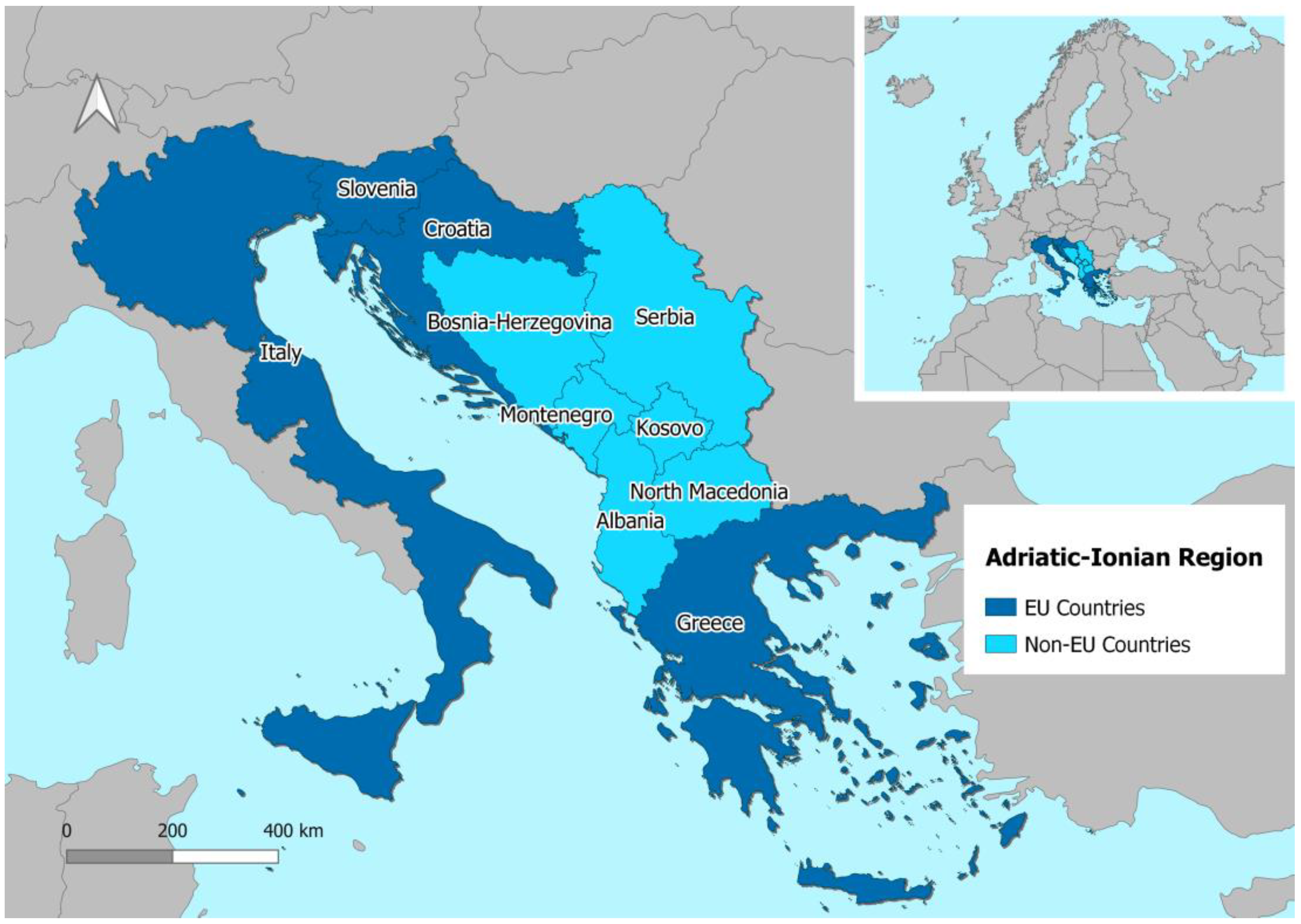
The application is related to the Adriatic and Ionian (AI) region (Figure 2); it is currently characterized by a high level of disparities between countries from the economic, political, and social perspectives, but also from point of view of infrastructural assets. Moreover, it includes both some EU countries (Italy, Slovenia, Croatia, and Greece) and non-EU ones (Bosnia-Herzegovina, Montenegro, Albania, North Macedonia, and Kosovo). The application is limited to road, rail, and maritime transportation, identified as the most relevant transportation modes for the purpose of our analysis and in relation to the considered case study. This section is organized as follows. Data sources used are briefly described in Section 4.1, accessibility analysis related to the current scenario is reported in Section 4.2, while spatial regression model estimation results are shown in Section 4.3. Gross Domestic Product per Capita (GDPC) forecast due to the TEN-T network extension in the AI region is finally reported in Section 4.4.

4.1. Data Source

The analysis focuses on a sample consisting of 225 NUTS-3 zones included in the AI region. For each zone, and neighboring zones where needed, several socioeconomic data have been collected. Particularly, zonal population ( P o p ), employment rate ( E M P R A T E ), and Gross Domestic Product per Capita ( G D P C ) come from worldwide [45], European [46,47], and National Statistical Offices [48,49,50] publicly available databases. The European Quality of Government Index ( E Q I ) has been directly taken by [44] for the European countries, while it has been estimated starting from World Bank data [51] for non-European ones. Transportation-related variables come from ad hoc macro-simulation transportation models related to road, rail, and maritime transportation developed for the AI region within the PTV VISUM software; the modelled multimodal network consists of about 60,000 nodes and 200,000 links, a quarter of which are related to rail transportation. Even though the focus is on the AI region, the model also includes 136 EU and non-EU zones to simulate the interaction with the former. All the data used for spatial modelling estimation refer to the base year of the analysis, i.e., 2017.

4.2. Current Scenario Accessibility Analysis

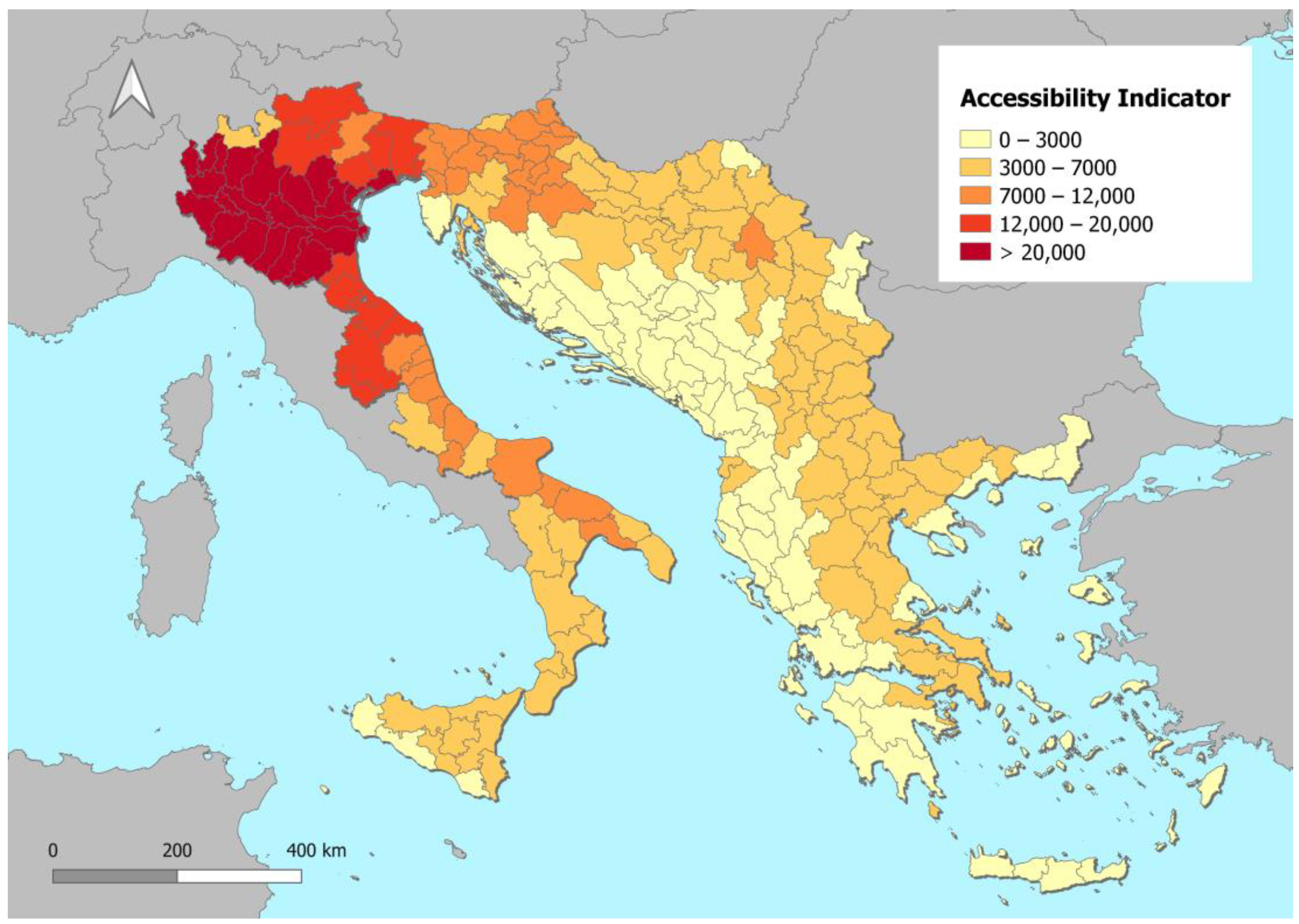
With reference to the current scenario, multimodal accessibility analysis results are shown in Figure 3. The map highlights an east–west accessibility pattern; the western part of the AI region (i.e., the one mainly composed by the Italian provinces) has an average accessibility level greater than the Balkan countries. This is mainly due to the greater performances of the existing Italian transportation infrastructural asset in relation to the Balkan one; high capillarity together with high multimodal network performances guarantee lower generalized travel costs and, subsequently, more opportunities for interaction for those living in this area. Moreover, with reference to Italy, it is worth noting a north–south accessibility pattern: the northern regions benefit from greater accessibility due to both a greater transportation network density and to their structural geographical location, i.e., geometrically more central in relation to the distribution of the European population than peripheral southern Italian areas.

4.3. Spatial Regression Model Estimations

As a preliminary step, the presence of spatial autocorrelation of the dependent variable (i.e., GDPC) has been probed, and the resulting Moran’s Index ( M I ) is equal to 0.92; this has been then tested against the one obtained by randomizing the sample through a Monte Carlo simulation (i.e., the one referring to a dataset with no spatial structure). The hypothesis that two MIs are statistically equal has been rejected (p-value < 0.001).
Results from the spatial regression model estimations using year 2017 cross-sectional data are reported in Table 1. A queen-based contiguity binary matrix W has been used, having a row-normalized weight and elements w i j 0 if zone i and zone j are neighbors, and w i j = 0 if vice versa. Moreover, a k-Nearest Neighbors criterion has been used to account for the presence of islands, which rely on maritime connection toward the land zones.
As expected, β 1 , β 2 , and β 3 coefficients measuring the direct impacts (i.e., not spatially lagged) of the independent variables on the dependent one are positive in all model specifications; an increase in the employment rate or in the quality of government or in the transportation accessibility of zone i generates an increase in the GDPC of the same zone. θ 2 and θ 3 coefficients measuring the spatially lagged impacts of E Q I and A C C , respectively, are highly statistically significant (p-value < 0.001) only in the SDM specification. They both have negative signs, highlighting the presence of a “spatial competition” effect between neighboring areas, for instance, an increase in the transportation accessibility in nearby zone j will negatively affect the GDPC of zone i due to both a potential greater attractiveness and a more competitive accessibility advantage of the former (zone j ). The SEM model has the λ coefficient, the one associated with the spatially lagged error, with a high statistical significance (p-value < 0.001), highlighting the presence of spatial effects not explicitly considered in this model specification, except in the error term. Furthermore, both the SEM and the SLX have higher intercepts with respect to the other estimated models and these are also highly statistically significant, indicating how both exclude important variables in their specification (for instance, the spatially lagged GDPC).
With the aim of identifying the model that fits best, a comparison through the Akaike Information Criterion (AIC) has been performed; the Spatial Durbin Model proved to be preferrable (i.e., lower AIC value) and it has been used for GDPC forecasting reported in Section 4.4. This is also proof of how spatial relationships between variables play a fundamental role in the economic impact assessment of transportation infrastructure; among all the estimated models, the SDM is the only one that considers the spatial effect of both the dependent ( G D P C ) and independent variables ( E M P R A T E , E Q I , A C C ), capturing the most complex spatial relationships between nearby areas, unlike the other model specifications.

4.4. GDPC Variation Forecast Due to the TEN-T Network Extension in the AI Region

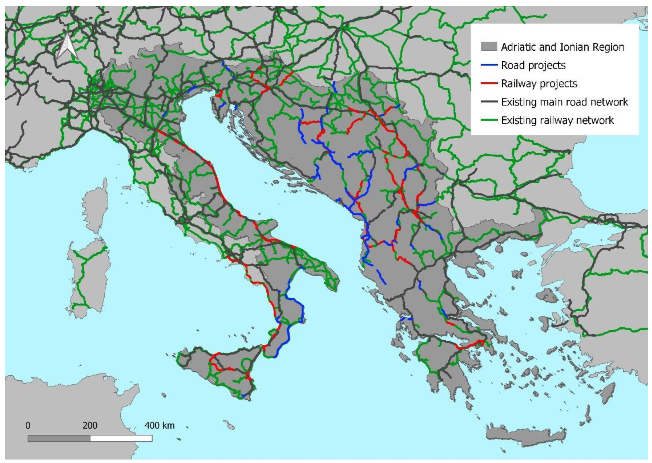
The simulated project scenario includes all the road and rail projects as per [52], extending the TEN-T network in the AI region, as reported in Figure 4.
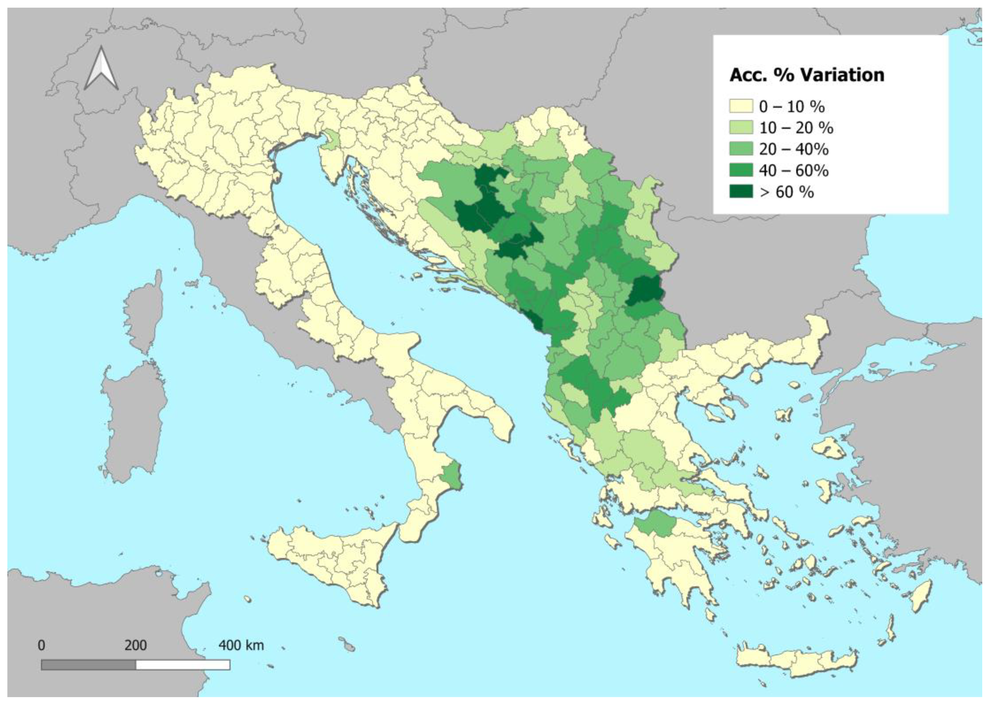
Results from the project scenario accessibility calculation are reported in Figure 5; the map shows how the greatest percentage variations are related to the Balkan area. This is in line with what might be expected, considering that most of the investments are located in the Western Balkans.
Considering the whole AI region, the average accessibility increase was found to be equal to +14% (see Table 2). It is worth noting that the coastal area of Bar (Montenegro), together with the surrounding ones, presents the highest benefit in terms of relative accessibility variation (+93.1%); this is due to important road (the Blu Highway, included in the Mediterranean TEN T Corridor) and railway projects located in the same area. The same goes for Bosnia-Herzegovina; this benefit was found to be on average a +37.8% accessibility increase, touching higher percentages where road and rail projects included both in the South East Europe Transport Observatory (SEETO) Corridor Vc or Route 2 are located. Serbia also benefits from a significant increase in accessibility (up to +62% variation), mainly due to the reconstruction and modernization of the railway line that is part of the Orient-Est/Med TEN-T corridor.
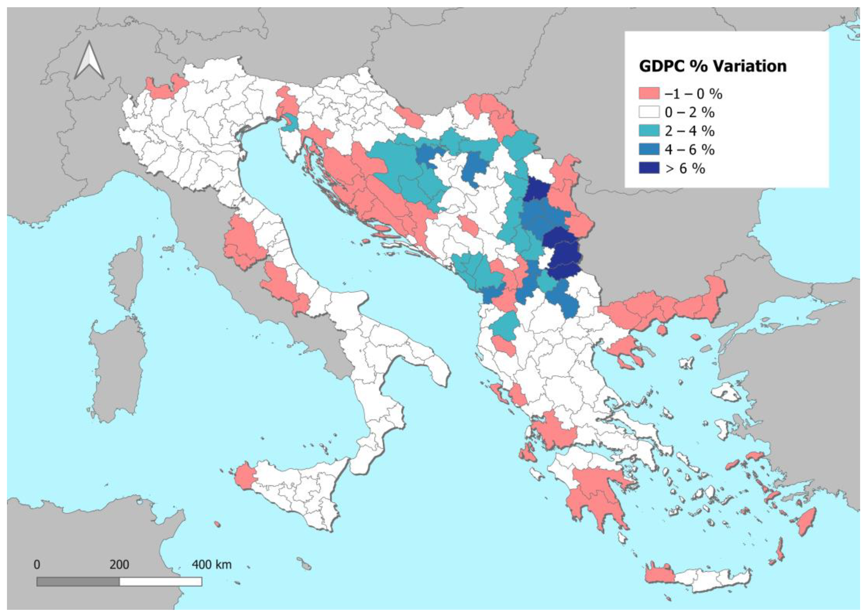
Taking these new zonal accessibility values as input, the estimated Spatial Durbin Model (see Section 4.3) has been used for GDPC forecasting. Results in terms of zonal GDPC percentage variations are reported in Figure 6; the map highlights how some areas experience a GDPC increase (blue-colored zones on which the darker is the blue, the higher is the GDPC % increase), while it decreases in some others (light red-colored areas).

5. Discussion

The estimated Gross Domestic Product per Capita (GDPC) percentage variation due to road and railway projects extending the TEN-T network in the Adriatic and Ionian (AI) region was found to be equal to +0.9% on average at the NUTS-3 level. Even though it is not directly comparable since it is context-specific, it is worth noting that the estimated value is in line with those previously obtained by other authors, for instance, [19], using a Spatial Durbin Model specification, stated that the Eastern European countries (including Estonia, Latvia, Lithuania, Poland, the Czech Republic, Slovakia, Hungary, Slovenia, Croatia, Romania, Bulgaria, and Greece) could benefit from the TEN-T core road corridors’ completion with a GDPC increase ranging from +0.9% to +1.3%. Apart from the average value, the GDPC percentage variation estimated in this study ranges between −0.8% and +10.2% at the NUTS-3 level for the AI region, where higher percentages are related to non-EU countries characterized by underdeveloped transportation networks (e.g., North Macedonia or Serbia). In fact, average National GDPC increases reported in Table 3 show that Western Balkans countries benefit from a +1.8% GDPC increase on average, unlike the EU countries, where the economic impacts are lower (+0.2% on average).
As was found from the modelling estimation, the spatially lagged effect on GDPC, i.e., the influence of the neighboring areas, is negative and can sometimes be predominant. The positive effect on GDPC given by (direct or indirect, i.e., through network effects) accessibility increases in the whole study area is sometimes overbalanced by negative spatially lagged effects, resulting in a GDPC positive variation polarization, mainly where interventions are located, to the detriment of the nearby zones.
For instance, Italy has an infrastructural enhancement on the Adriatic and Tyrrhenian corridors, resulting both in a positive GDPC variation on coastal areas (up to to +0.8%) and a slight GDPC decrease in the nearby Apennine hinterland regions (up to −0.1%). Another example is related to inland areas of Bosnia-Herzegovina and Croatian coastal areas; while the former benefit from a +2.7% GDPC increase on average, the latter have a decrease of up to −0.3% and −0.4%, respectively. In addition, some Albanian areas experience negative economic impacts since they are geographically located in an “investment shadow area”; they are surrounded by important infrastructural enhancements, but they do not benefit from them, as their rail and road network is not well-integrated and connected.
The potential conflict between direct and spatial spillover effects has also been highlighted by [53]; as in this study, they confirm the possibility of having negative spillover effects caused by increased territorial competition exceeding direct positive ones, therefore suggesting to policymakers that these impacts should always be taken into account in transportation project appraisal [54]. However, there are other studies (for instance, [55]) finding neither positive direct nor negative spillover effects of transportation investment on the regional growth, arguing that other factors such as investment in research and development or regional migration rates are far more important than transportation-related variables in explaining regional economic welfare.
In this study, the statistical significance of both socioeconomic (i.e., the employment rate E M P R A T E ) and political-context-related variables (i.e., the quality of government index E Q I ) in estimating GDPC has been proven, suggesting how policies and decisions affecting contexts other than real-world transportation could positively impact regional economies. In particular, a positive impact on GDPC can be achieved by acting on different systems (for example, the socioeconomic, the political, or the transportation systems), and different policies, not limited to transportation, should be evaluated in a comparative way, especially with reference to those areas where investments in transportation infrastructure are not cost-efficient due to the topography of the territory in which they would be located.

6. Conclusions

In this paper, a modelling framework is proposed to assess the spatial economic impacts of transportation infrastructure investments; it combines spatial econometric techniques with transportation accessibility analysis to estimate the variation of zonal Gross Domestic Product per Capita (GDPC), assumed as a proxy of the economic growth. The application to the Adriatic and Ionian (AI) region case study is presented; among its peculiarities, the area includes both EU (Italy, Slovenia, Croatia, and Greece) and non-EU countries (Bosnia-Herzegovina, Montenegro, Albania, North Macedonia, and Kosovo) and is characterized by high disparities in terms of infrastructural assets.
The estimated models allowed us to prove the importance of considering the spatial relationship between variables in transportation infrastructure economic impact evaluation. The Spatial Durbin Model specification was found to be the one that best fits; among those tested, it is the only model specification able to capture complex spatial relationships between nearby areas, considering spatially lagged effects generated from both the dependent ( G D P C ) and independent variables (i.e., the employment rate E M P R A T E , the quality of government index E Q I , and the transportation accessibility indicator A C C ).
Finally, the estimated SDM model has been used to forecast GDPC variation due to road and rail investments foreseen in the AI region by supranational strategies, as per [52]. It allows us to first quantitatively measure the zonal GDPC variation due to an increased multimodal transportation accessibility, and second it allows us to outline where current economic disparities tend to be bridged up (i.e., mainly along the foreseen extensions of the TEN-T corridors) and where not, suggesting the need of new policies to fill these gaps.
Among the limitations of this research, it is worth mentioning the modelling estimation using cross-sectional data. The use of panel data would have given more robust estimates; however, to the best of our knowledge, longitudinal data related to variables considered in this study are not publicly available for Western Balkan countries. Moreover, spatial modelling estimations have been performed using data related to 2017, i.e., a few years before disruptive crises such as the COVID-19 pandemic and the Ukraine war happened; these had and will have impacts on regional economies that the model fails to capture by its very nature.
Another limitation is that the simulated project scenario considers only road and railway projects in the AI region, ignoring those located in neighboring countries; results for the edge zones must be therefore carefully evaluated. Future research should address these limitations in order to obtain, on the one hand, more accurate estimates, and on the other, more reliable results for the bordering areas to draw up wider considerations. Moreover, a possible follow-up to this study could evaluate the impact on regional economies of investments in transportation nodes that are not considered in this study. This would be possible by adapting the proposed methodology by introducing a service frequency variable in the accessibility indicator formulation, consequently simulating the impact that would be generated by increases in service frequencies allowed by nodal (such as ports or airports) capacity enhancements.

Author Contributions

Conceptualization, P.C.; methodology, F.D.F. and F.S.; formal analysis, F.D.F. and F.S.; data curation, F.D.F. and A.C.M.; writing—original draft preparation, F.D.F.; writing—review and editing, F.D.F. and P.C.; visualization, F.D.F.; project administration, P.C. All authors have read and agreed to the published version of the manuscript.

Funding

This study has been carried out within the framework of the TRIBUTE Project (ADRION 1239-CUP: D45H20000190004) funded by the INTERREG V-B Adriatic–Ionian ADRION Programme.

Institutional Review Board Statement

Not applicable.

Informed Consent Statement

Not applicable.

Data Availability Statement

Most datasets used and/or analyzed during this study are available on reasonable request from the corresponding author.

Conflicts of Interest

The authors declare no conflict of interest.

References

  1. Thomas, I. Transportation Networks and the Optimal Location of Human Activities: A Numerical Geography Approach; Edward Elgar Publishing: Cheltenham, UK, 2002. [Google Scholar]
  2. Cascetta, E.; Coppola, P.; Velardi, V. High-Speed Rail Demand: Before-and-After Evidence from the Italian Market. disP-Plan. Rev. 2013, 49, 51–59. [Google Scholar] [CrossRef] [Green Version]
  3. Murray, A.T.; Davis, R.; Stimson, R.J.; Ferreira, L. Public Transportation Access. Transp. Res. Part D Transp. Environ. 1998, 3, 319–328. [Google Scholar] [CrossRef] [Green Version]
  4. Spiekermann, K.; Neubauer, J. European Accessibility and Peripherality: Concepts, Models and Indicators; Report 2002; Nordregio: Stockholm, Sweden, 2002. [Google Scholar]
  5. Sánchez-Mateos, H.S.M.; Givoni, M. The accessibility impact of a new High-Speed Rail line in the UK—A preliminary analysis of winners and losers. J. Transp. Geogr. 2012, 25, 105–114. [Google Scholar] [CrossRef]
  6. Banister, D.; Berechman, Y. Transport investment and the promotion of economic growth. J. Transp. Geogr. 2001, 9, 209–218. [Google Scholar] [CrossRef]
  7. EC—DG REGIO. Guide to Cost-Benefit Analysis of Investment Projects for Cohesion Policy 2014–2020; EC—DG REGIO: Etterbeek, Belgium, 2015. [Google Scholar]
  8. Rokicki, B.; Stępniak, M. Major transport infrastructure investment and regional economic development—An accessibility-based approach. J. Transp. Geogr. 2018, 72, 36–49. [Google Scholar] [CrossRef]
  9. Cascetta, E.; Cartenì, A.; Henke, I.; Pagliara, F. Economic growth, transport accessibility and regional equity impacts of high-speed railways in Italy: Ten years ex post evaluation and future perspectives. Transp. Res. Part A Policy Pract. 2020, 139, 412–428. [Google Scholar] [CrossRef] [PubMed]
  10. Delft, C.E.; Directorate-General for Mobility and Transport (European Commission); van Essen, H.; van Wijngaarden, L.; Schroten, A.; Sutter, D.; Bieler, C.; Maffii, S.; Brambilla, M.; Fiorello, D.; et al. Handbook on the External Costs of Transport: Version 2019–1.1; Publications Office of the European Union: Luxembourg, 2020. [Google Scholar]
  11. Boardman, A.E.; Greenberg, D.H.; Vining, A.R.; Weimer, D.L. Cost-Benefit Analysis: Concepts and Practice; Cambridge University Press: Cambridge, UK, 2017. [Google Scholar]
  12. De Rus, G. The BCA of HSR: Should the Government Invest in High Speed Rail Infrastructure? J. Benefit-Cost Anal. 2011, 2, 1–28. [Google Scholar] [CrossRef] [Green Version]
  13. Willis, K.; Garrod, G.; Harvey, D. A review of cost–benefit analysis as applied to the evaluation of new road proposals in the U.K. Transp. Res. Part D Transp. Environ. 1998, 3, 141–156. [Google Scholar] [CrossRef]
  14. Bröcker, J.; Korzhenevych, A.; Schürmann, C. Assessing spatial equity and efficiency impacts of transport infrastructure projects. Transp. Res. Part B Methodol. 2010, 44, 795–811. [Google Scholar] [CrossRef]
  15. Adler, M.D. Cost-Benefit Analysis and Distributional Weights: An Overview; Duke University: Durham, NC, USA, 2013. [Google Scholar]
  16. Robson, E.N.; Wijayaratna, K.P.; Dixit, V.V. A review of computable general equilibrium models for transport and their applications in appraisal. Transp. Res. Part A Policy Pract. 2018, 116, 31–53. [Google Scholar] [CrossRef]
  17. Chen, Z. Measuring the regional economic impacts of high-speed rail using a dynamic SCGE model: The case of China. Eur. Plan. Stud. 2019, 27, 483–512. [Google Scholar] [CrossRef]
  18. Haddad, E.A.; Hewings, G.; Perobelli, F.S.; Dos Santos, R.A.C. Regional Effects of Port Infrastructure: A Spatial CGE Application to Brazil. Int. Reg. Sci. Rev. 2010, 33, 239–263. [Google Scholar] [CrossRef]
  19. Goldmann, K.; Wessel, J. TEN-T corridors–Stairway to heaven or highway to hell? Transp. Res. Part A Policy Pract. 2020, 137, 240–258. [Google Scholar] [CrossRef]
  20. Crescenzi, R.; Di Cataldo, M.; Rodríguez-Pose, A. Government quality and the economic returns of transport infrastructure investment in european regions. J. Reg. Sci. 2016, 56, 555–582. [Google Scholar] [CrossRef]
  21. Maucorps, A.; Jestl, S.; Römisch, R. The Effects of the EU Cohesion Policy on Regional Economic Growth: Using Structural Equation Modelling for Impact Assessment; Vienna Institute for International Economic Studies: Wien, Austria, 2020. [Google Scholar]
  22. Jiang, X.; He, X.; Zhang, L.; Qin, H.; Shao, F. Multimodal transportation infrastructure investment and regional economic development: A structural equation modeling empirical analysis in China from 1986 to 2011. Transp. Policy 2017, 54, 43–52. [Google Scholar] [CrossRef]
  23. Chen, Z.; Haynes, K. Spatial Impact of Transportation Infrastructure: A Spatial Econometric CGE Approach; Springer International Publishing: Berlin/Heidelberg, Germany, 2015; pp. 163–186. [Google Scholar]
  24. LeSage, J.; Pace, R.K. Introduction to Spatial Econometrics; Chapman and Hall/CRC: New York, NY, USA, 2009. [Google Scholar]
  25. Bolduc, D.; Laferrière, R.; Santarossa, G. Spatial Autoregressive Error Components in Travel Flow Models: An Application to Aggregate Mode Choice. In New Directions in Spatial Econometrics; Anselin, L., Florax, R.J.G.M., Eds.; Springer: Berlin/Heidelberg, Germany, 1995; pp. 96–108. [Google Scholar]
  26. Haider, M.; Miller, E.J. Effects of Transportation Infrastructure and Location on Residential Real Estate Values: Application of Spatial Autoregressive Techniques. Transp. Res. Rec. J. Transp. Res. Board 2000, 1722, 1–8. [Google Scholar] [CrossRef]
  27. Hackney, J.K.; Bernard, M.; Bindra, S.; Axhausen, K.W. Predicting road system speeds using spatial structure variables and network characteristics. J. Geogr. Syst. 2007, 9, 397–417. [Google Scholar] [CrossRef] [Green Version]
  28. Ibeas, Á.; Cordera, R.; Dell’Olio, L.; Coppola, P.; Dominguez, A. Modelling transport and real-estate values interactions in urban systems. J. Transp. Geogr. 2012, 24, 370–382. [Google Scholar] [CrossRef] [Green Version]
  29. Cordera, R.; Coppola, P.; Dell’Olio, L.; Ibeas, Á. Is accessibility relevant in trip generation? Modelling the interaction between trip generation and accessibility taking into account spatial effects. Transportation 2017, 44, 1577–1603. [Google Scholar] [CrossRef]
  30. Cordera, R.; Coppola, P.; Dell’Olio, L.; Ibeas, Á. The impact of accessibility by public transport on real estate values: A comparison between the cities of Rome and Santander. Transp. Res. Part A Policy Pract. 2018, 125, 308–319. [Google Scholar] [CrossRef]
  31. Lopes, S.; Brondino, N.C.M.; Da Silva, A.N.R.; Da Silva, A.R. GIS-Based Analytical Tools for Transport Planning: Spatial Regression Models for Transportation Demand Forecast. ISPRS Int. J. Geo-Inf. 2014, 3, 565–583. [Google Scholar] [CrossRef] [Green Version]
  32. Zeng, C.; Song, Y.; Cai, D.; Hu, P.; Cui, H.; Yang, J.; Zhang, H. Exploration on the spatial spillover effect of infrastructure network on urbanization: A case study in Wuhan urban agglomeration. Sustain. Cities Soc. 2019, 47, 101476. [Google Scholar] [CrossRef]
  33. Yu, N.; de Jong, M.; Storm, S.; Mi, J. Spatial spillover effects of transport infrastructure: Evidence from Chinese regions. J. Transp. Geogr. 2013, 28, 56–66. [Google Scholar] [CrossRef]
  34. Gutiérrez, J.; Condeço-Melhorado, A.; Martín, J.C. Using accessibility indicators and GIS to assess spatial spillovers of transport infrastructure investment. J. Transp. Geogr. 2009, 18, 141–152. [Google Scholar] [CrossRef]
  35. Lopez, E.; Monzón, A.; Ortega, E.; Quintana, S.M. Assessment of Cross-Border Spillover Effects of National Transport Infrastructure Plans: An Accessibility Approach. Transp. Rev. 2009, 29, 515–536. [Google Scholar] [CrossRef]
  36. Moreno, R.; López-Bazo, E. Returns to Local and Transport Infrastructure under Regional Spillovers. Int. Reg. Sci. Rev. 2007, 30, 47–71. [Google Scholar] [CrossRef]
  37. Geurs, K.T.; van Wee, B. Accessibility evaluation of land-use and transport strategies: Review and research directions. J. Transp. Geogr. 2004, 12, 127–140. [Google Scholar] [CrossRef]
  38. Reggiani, A. Accessibility, Trade and Locational Behaviour; Routledge: London, UK, 2019. [Google Scholar]
  39. Coppola, P.; Nuzzolo, A. Changing accessibility, dwelling price and the spatial distribution of socio-economic activities. Res. Transp. Econ. 2011, 31, 63–71. [Google Scholar] [CrossRef] [Green Version]
  40. Ortega, E.; Lopez, E.; Monzón, A. Territorial cohesion impacts of high-speed rail at different planning levels. J. Transp. Geogr. 2012, 24, 130–141. [Google Scholar] [CrossRef]
  41. Monzón, A.; Ortega, E.; López, E. Efficiency and spatial equity impacts of high-speed rail extensions in urban areas. Cities 2013, 30, 18–30. [Google Scholar] [CrossRef] [Green Version]
  42. Cascetta, E. Transportation Systems Analysis: Models and Applications; Springer: Boston, MA, USA, 2009. [Google Scholar]
  43. Moran, P.A.P. The Interpretation of Statistical Maps. J. R. Stat. Soc. Ser. B Methodol. 1948, 10, 243–251. [Google Scholar] [CrossRef]
  44. Charron, N.; Lapuente, V.; Annoni, P. Measuring quality of government in EU regions across space and time. Pap. Reg. Sci. 2019, 98, 1925–1953. [Google Scholar] [CrossRef]
  45. World Bank National Accounts Data, and OECD National Accounts Data Files. GDP (Constant 2015 US$). Available online: https://data.worldbank.org/indicator/NY.GDP.MKTP.KD (accessed on 7 August 2022).
  46. European Commission-ARDECO Online-Knowledge for Policy. Available online: https://knowledge4policy.ec.europa.eu/territorial/ardeco-online_en (accessed on 7 August 2022).
  47. Eurostat-Statistics. Available online: https://ec.europa.eu/eurostat/databrowser/view/NAMA_10R_3GDP/default/table?lang=en (accessed on 7 August 2022).
  48. Agency for Statistics of Bosnia and Herzegovina-Statistics. Available online: https://bhas.gov.ba/?lang=en (accessed on 13 August 2022).
  49. Kosovo Agency of Statistics-Statistics. Available online: https://askdata.rks-gov.net/pxweb/en/ASKdata/ (accessed on 13 August 2022).
  50. INSTAT-Albanian Institute of Statistics-Statistics. Available online: https://www.instat.gov.al/en/ (accessed on 13 August 2022).
  51. World Bank—Worldwide Governance Indicators (WGI) Database. Available online: http://info.worldbank.org/governance/wgi/ (accessed on 24 August 2022).
  52. European Commission (2021) Proposal for a Regulation of the European Parliament and of the Council on Union Guidelines for the Development of the Trans-European Transport Network, Amending Regulation (EU) 2021/1153 and Regulation (EU) No 913/2010 and Repealing Regulation (EU) 1315/2013. Available online: https://eur-lex.europa.eu/legal-content/EN/ALL/?uri=COM%3A2021%3A812%3AFIN (accessed on 11 July 2022).
  53. Del Bo, C.F.; Florio, M. Infrastructure and Growth in a Spatial Framework: Evidence from the EU regions. Eur. Plan. Stud. 2012, 20, 1393–1414. [Google Scholar] [CrossRef]
  54. Elburz, Z.; Nijkamp, P.; Pels, E. Public infrastructure and regional growth: Lessons from meta-analysis. J. Transp. Geogr. 2017, 58, 1–8. [Google Scholar] [CrossRef]
  55. Crescenzi, R.; Rodríguez-Pose, A. Infrastructure and regional growth in the European Union. Pap. Reg. Sci. 2012, 91, 487–513. [Google Scholar] [CrossRef]
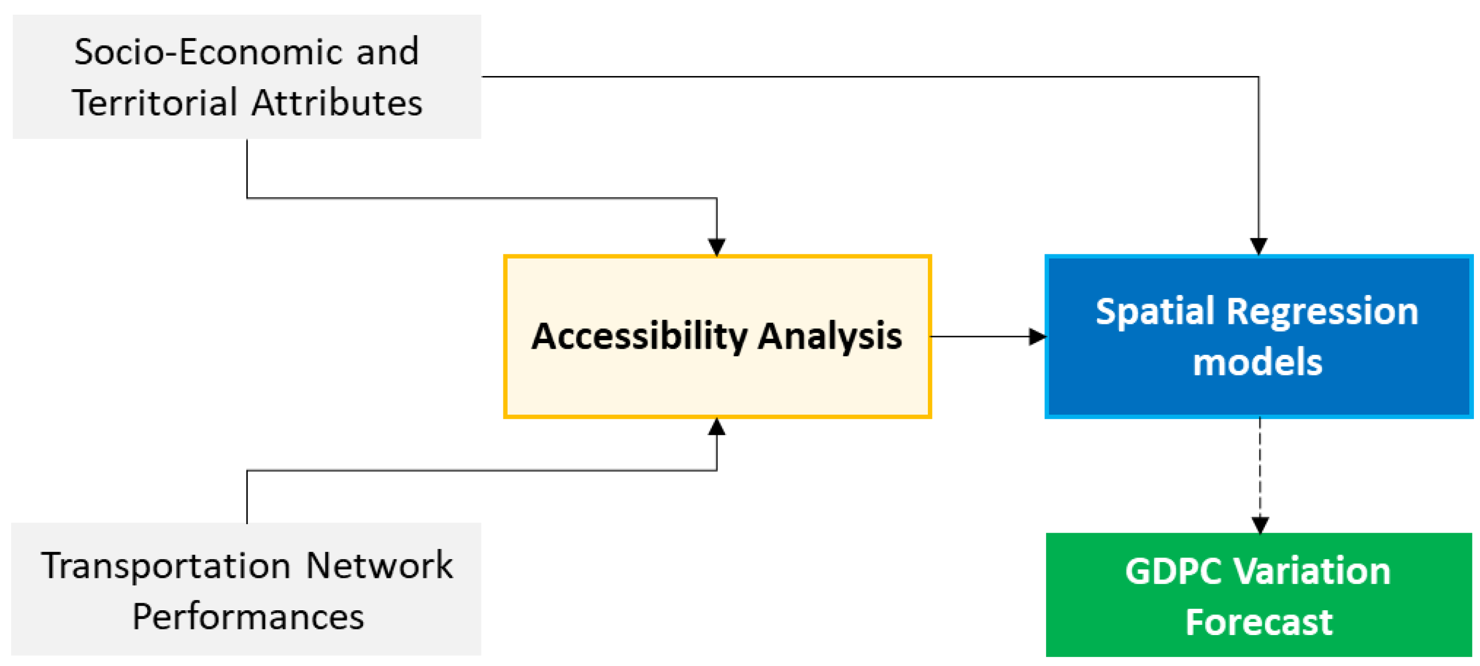
Figure 1. Simplified depiction of the proposed methodological approach.
Sustainability 15 05126 g001
Figure 2. Adriatic and Ionian region location map.
Sustainability 15 05126 g002
Figure 3. Accessibility indicator [*10,000] map related to the current scenario.
Sustainability 15 05126 g003
Figure 4. Existing main road and railway networks, together with main road and railway projects in the Adriatic and Ionian region, as per [52].
Sustainability 15 05126 g004
Figure 5. Accessibility indicator percentage variation between current and project scenario.
Sustainability 15 05126 g005
Figure 6. GDPC percentage variation between current and project scenario.
Sustainability 15 05126 g006
Table 1. Results from spatial regression model (SDM, SAR, SLX, SEM) estimations.
SDMSARSLXSEM
ln E M P R A T E ( β 1 )0.161 ***0.126 **0.1150.150 **
E Q I ( β 2 )0.402 ***0.226 ***0.414 ***0.468 ***
A C C ( β 3 )0.262 ***0.0440.263 *0.292 ***
W   ·   ln E M P R A T E ( θ 1 )−0.131 0.139
W   ·   E Q I ( θ 2 )−0.241 *** 0.244 *
W   ·   A C C ( θ 3 )−0.231 *** −0.009
α i 2.040 ***2.497 ***9.102 ***9.206 ***
𝜌0.800 ***0.711 ***
λ 0.808 ***
Observations225225225225
Pseudo-R20.9040.891 0.901
Multiple R2 0.730
Log Likelihood−0.45−13.93−116.1−3.84
Akaike Inf. Crit.18.9139.86248.119.69
LR Test231.2 ***211.4 *** 231.6 ***
Note: *, **, and *** indicate statistical significance at the 10%, 5%, and 1% levels, respectively.
Table 2. Accessibility values [*10,000] and absolute/relative changes between current and project scenario.
CountryAccessibility Values (*10,000)Accessibility Changes
Current ScenarioProject ScenarioAbsoluteRelativeRelative NUTS 3 Range [Min–Max]
Albania2138277163429.6%[12.4–54.7%]
Bosnia-Herzegovina2428334491637.8%[4.5–93.0%]
Croatia533357093767.1%[1.0–20.9%]
Greece246026341757.1%[0.0–42.0%]
Italy13,67113,8651941.4%[0.1–30.2%]
Kosovo39204972105226.8%[13.7–39.8%]
Montenegro1580232174146.9%[21.5–93.1%]
North Macedonia42555540128530.2%[15.6–45.6%]
Serbia41805264108425.9%[2.6–62.1%]
Slovenia939197483563.8%[0.8–15.7%]
Adriatic–Ionian Average6735721648114.0%[0.0–93.1%]
Table 3. GDPC values [€] and absolute/relative changes between current and project scenario.
CountryGDPC Values (€)GDPC Changes
Current ScenarioProject ScenarioAbsoluteRelativeRelative NUTS 3 Range [Min–Max]
Albania34953540451.3%[−0.5–4.1%]
Bosnia-Herzegovina45744635611.3%[−0.3–4.5%]
Croatia99409993530.5%[−0.4–3.0%]
Greece13,51613,539230.2%[−0.3–2.0%]
Italy26,33826,378400.2%[−0.1–0.8%]
Kosovo34823543601.7%[−0.1–4.2%]
Montenegro69086998901.3%[−0.4–3.2%]
North Macedonia449746451493.3%[0.9–10.1%]
Serbia43904479902.0%[−0.8–10.2%]
Slovenia18,22918,3861570.9%[−0.2–3.2%]
Adriatic–Ionian Average14,17714,235580.9%[−0.8–10.2%]
EU Countries inside the AI Region average19,32119,367460.2%[−0.4–3.2%]
non-EU Countries inside the AI Region average44824562801.8%[−0.8–10.2%]
Disclaimer/Publisher’s Note: The statements, opinions and data contained in all publications are solely those of the individual author(s) and contributor(s) and not of MDPI and/or the editor(s). MDPI and/or the editor(s) disclaim responsibility for any injury to people or property resulting from any ideas, methods, instructions or products referred to in the content.