A Polynomial Chaos Expansion Method for Mechanical Properties of Flexoelectric Materials Based on the Isogeometric Finite Element Method

Abstract

The paper proposes a method for analyzing the mechanical properties of flexoelectric materials based on the isogeometric finite element method (IGA-FEM) and polynomial chaos expansion (PCE). The method discretizes the flexoelectric governing equations utilizing the B-spline shape functions that satisfy the continuity requirement to obtain the mechanical properties (electric potential) of the material. To obtain a mechanical property with different input parameters, we choose the truncated pyramid model as the object of study, and use IGA-FEM and PCE to solve different single uncertain parameters, including independent Young’s modulus and uniformly distributed force, and two kinds of flexoelectric constants, respectively. Numerical examples are presented to bear out the accuracy and viability of the proposed methodology.

1. Introduction

Mashkevich and Tolpygo proposed flexoelectricity in solids in the 1950s [1], but flexoelectric effects were weak for bulk crystalline materials, so flexoelectricity received limited attention in the early period. With the development of nanotechnology, significant strain gradients may now be seen on short-length scales. Flexoelectricity is becoming a new way of understanding of size-dependent phenomena [2]. In contrast to piezoelectric materials, which exhibit linear electrical polarization with mechanical strain, the flexoelectric materials display gradient-dependent electrical polarization with mechanical strain [3]. Flexoelectricity is a more prevalent electromechanical coupling mechanism than piezoelectricity since it may potentially occur in practically any dielectric, even those with centrosymmetric crystal structures [4]. The interested reader may read the references [5,6] for further current reviews on flexoelectricity.

In the numerical analysis of dielectric solids (e.g., piezoelectric and flexoelectric), the parameters of the materials considered in most studies are deterministic [7,8,9,10]. However, the input parameters in real engineering are generally highly uncertain and there are limitations in the parameter estimation of the model, which leads us to make erroneous decisions on some real engineering problems [11,12,13,14]. The quantization of uncertainty in engineering is to obtain the statistical characteristics of response by studying the uncertainty of input parameters to the model. Approaches to uncertainty analysis, such as Monte Carlo simulations (MCs) [15], stochastic spectral methods [16,17], and perturbation techniques [18,19], typically quantify the statistical characteristics (mathematical expectation and standard deviation) of the system response. As the modeling requirements increase, the simulation model of the objective becomes extremely complex, the computation time for uncertainty quantification increases, and the efficiency decreases. Traditional MCs methods require a significant number of samples and model observations for uncertainty quantification, making it difficult to address some of the more complex problems [20]. Surrogate models can be used to replace complex analytical or computational models by using a basic polynomial function to establish input-output relationships [21,22]. The development of an appropriate surrogate model can provide the required model observations at a rational computational cost, beyond the limitations of conventional calculations.

The polynomial chaos expansion (PCE) method is an efficient way to quantify uncertainty because it is computationally inexpensive [23]. The expression of the unknown function of the response is obtained by a series of orthogonal polynomials, and the polynomial surrogate model about the random input parameters is established by solving for the coefficients of the components in the unknown function [24,25,26]. The fact that these polynomials are orthogonal to each other with respect to the joint probability density function of the inputs simplifies computation. There are various methods to solve the PCE coefficients, such as non-intrusive and intrusive methods. Implementing the intrusive method in real engineering issues is challenging and time-consuming since it necessitates changing the code for the governing equations to complete for uncertainty quantification [27]. Another non-intrusive method is appropriate for the majority of issues and does not require a clear understanding of the governing equations. As a result, the target problem may be characterized as a “black box” problem where observations can be made utilizing a variety of input variable samples [28]. The non-intrusive methods are classified into two main streams: projection methods [29] and regression methods [30,31], and regression methods to solve the PCE coefficients are very efficient [32] and became the most widely available solution method.

Isogeometric analysis (IGA), a Finite Element Method (FEM) extension, is a critical milestone in the development of computational mechanics [33]. The IGA has the advantage of using Non-Uniform Rational B-spline basis functions to discrete partial differential equations, allowing engineers to perform numerical analysis directly from Computer-Aided Design (CAD), reducing the burden of meshing while remaining geometrically accurate [34,35]. The IGA has rapidly expanded to a wide range of engineering applications such as elasticity [36], electromagnetics [37], fluid flow [38], acoustic problems [39,40], and optimization problems [41,42,43,44,45,46] since its inception. Jahanbin and Rahman [47] have made significant contributions to the stochastic isogeometric analysis (SIGA) of linear elasticity of high-dimensional functions in the growth of engineering applications of uncertainty quantification. Liu et al. [48] presented a new technique for real engineering problems based on reduced basis vectors in the stochastic isogeometric analysis (SIGA). IGA can provide the $C^1$ continuity requirement, which satisfies the continuity requirement of the fourth order partial differential equations (PDEs) for the flexoelectricity considered in this paper. Therefore, the IGA-FEM is chosen in this paper to obtain the mechanical properties of the flexoelectric structure.

In this paper, we propose a polynomial chaos expansion isogeometric FEM (PCE-IGA-FEM) to perform mechanical properties analysis for flexoelectric materials. This paper mainly makes the following two contributions:

1.

IGA-FEM is employed to analyze mechanical properties of flexoelectric materials.

2.

PCE is adapted to accelerate mechanical properties analysis for flexoelectric materials with different single uncertain parameters.

The remaining sections of the paper are structured as follows. Section 2 discusses the principles of PCE in the quantification of uncertainty. Section 3 introduce the fourth-order partial differential equations in flexoelectricity. Section 4 outlines the fundamental concepts of the IGA-FEM. Section 5 provides several numerical examples to validate the PCE method for flexoelectric structures, followed by Section 6 conclusions.

2. The PCE Fundamental Theory

PCE is an essential surrogate model strategy that represents the scalar model output y by expanding a series of orthogonal polynomials in the n-dimensional input parameters $\mathbf{r}=(r_1,r_2,\dots ,r_n)$. For any orthogonal condition of $i\ne j$, the inner product of arbitrary two functions and probability density function $\mathcal{P}\left(\mathbf{r}\right)$ provided by ${\psi }_i\left(\mathbf{r}\right)$ and ${\psi }_j\left(\mathbf{r}\right)$ that is [20]

$$\begin{array}{c}\hfill \begin{array}{c}\hfill \int {\psi }_i\left(\mathbf{r}\right){\psi }_j\left(\mathbf{r}\right)\mathcal{P}\left(\mathbf{r}\right)\mathrm{d}\mathbf{r}=w_i{\delta }_{ij}\end{array}\end{array}$$

(1)

when $i=j$, the Kronecker symbol ${\delta }_{ij}$ is one, otherwise it is zero, and $w_i$ is the weight. To simplify computations, the orthogonal polynomial, also known as the standard orthogonal polynomial, normalizes the probability density function so that $w_i$ equals 1 when $i=j$. Thus, the output function $y\left(\mathbf{r}\right)$ can be obtained as

$$\begin{array}{c}\hfill \begin{array}{c}\hfill y\left(\mathbf{r}\right)=\sum _{\mathbf{\alpha }\in {\mathbb{N}}^n}{c}_{\mathbf{\alpha }}{\Psi }_{\mathbf{\alpha }}\left(\mathbf{r}\right)\end{array}\end{array}$$

(2)

where $c_{\alpha }$ are the coefficients of the unknown polynomial. Multivariate orthogonal polynomials ${\Psi }_{\mathbf{\alpha }}$ are created by taking the tensor product of univariate orthogonal polynomials, which is defined as

$$\begin{array}{c}\hfill {\Psi }_{\mathbf{\alpha }}=\prod _{i=1}^n{\psi }_{\mathbf{\alpha }}\left(r_i\right)\end{array}$$

(3)

and $\mathbf{\alpha }=({\alpha }_1,{\alpha }_2,\dots ,{\alpha }_n)$ denote the exponents of the polynomial basis where ${\alpha }_i(i\in [1,n])$ represents the order of the respective parameter $r_i$ in the polynomial term. For the probability density functions of various distributions, there are several forms of orthogonal polynomials. The Legendre polynomials are orthogonal to the uniform distribution, while Hermite polynomials are equivalent to popular probability density functions like the Gaussian distribution.

Table 1. The probability density functions for four typical forms of orthogonal polynomials [49].

Distribution of Random Parameter	Type	Interval
Uniform	Legendre	$[a,b]$
Normal	Hermite	$(-\infty ,+\infty )$
Beta	Jacobi	$[a,b]$
Gamma	Laguerre	$(0,+\infty )$

lists the four most prevalent orthogonal polynomials.

The PCE representation in Equation (2) is sometimes reduced in actual applications to simplify the calculation and keep a smaller set of coefficients for training [20]. The standard truncation approach for PCE is

$$\begin{array}{c}\hfill \begin{array}{c}\hfill \mathcal{A}{}^{p,n}\equiv \{\mathbf{\alpha }\in {\mathbb{N}}^n:{∥\mathbf{\alpha }∥}_1\le p\},\end{array}\end{array}$$

(4)

Most of the time, the overall degree of PCE stays within the bounds of the stated order p [50]. The dimension of truncated PCE can be written as

$$\begin{array}{c}\hfill N=\left(\begin{array}{c}n+p\\ p\end{array}\right)=(n+p)!/(n!p!).\end{array}$$

(5)

The PCE coefficient $c_{\alpha }$ can be calculated in a variety of ways. In this paper, we seek to solve this coefficient by solving a least-squares minimization problem and using the most popular collocation approach. This approach minimizes the square of the Euclidean norm between the PCE and the solution $\mathrm{U}={\left\{{\left\{f\left(\mathbf{r}\right)\right\}}_{z=1}^Z\right\}}^{\mathrm{T}}$ by using Z random samples (collocation points). The orthogonal matrix and coefficient vector are [51]

$$\begin{array}{c}\hfill \Psi =\left. [\begin{array}{ccc}{\Psi }_0\left({\mathbf{r}}^1\right)& \dots & {\Psi }_{N-1}\left({\mathbf{r}}^1\right)\\ ·& & ·\\ ·& & ·\\ ·& & ·\\ {\Psi }_0\left({\mathbf{r}}^Z\right)& \dots & {\Psi }_{N-1}\left({\mathbf{r}}^Z\right)\end{array}\right]\mathrm{and}\mathbf{c}=\left\{\begin{array}{c}{c}_0\\ ·\\ ·\\ ·\\ c_{N-1}\end{array}\right\}.\end{array}$$

(6)

The PCE coefficient vector expression is

$$\begin{array}{c}\hfill \mathbf{c}={\left({\mathsf{\Psi }}^{\mathrm{T}}\mathsf{\Psi }\right)}^{-1}{\mathsf{\Psi }}^{\mathrm{T}}\mathrm{U}.\end{array}$$

(7)

In this paper, all random parameters satisfy Gaussian distribution, corresponding to Hermite orthogonal polynomials. Here, a one-dimensional random parameter is used to illustrate the recurrence relation of Hermite orthogonal polynomials, which is defined as

$$\begin{array}{c}\hfill {\Psi }_{\alpha }\left(r\right)=\frac{1}{{(-1)}^{\alpha }{e}^{-\frac{r^2}{2}}}\frac{d^{\alpha }}{d{r}^{\alpha }}\left. [e^{-\frac{r^2}{2}}\right]=\alpha !\sum _{k=0}^{[\alpha /2]}{(-1)}^k\frac{1}{k!2^k(\alpha -2k)!}{r}^{\alpha -2k}\end{array}$$

(8)

where $\left[\frac{\alpha }{2}\right]$ is the biggest number that is either smaller than or equal to $\frac{\alpha }{2}$. A one-dimensional random parameter is represented by the symbol r. The mathematical equation for the general recurrence of the Hermite orthogonal polynomial is

$$\begin{array}{c}\hfill {\Psi }_{\alpha +1}\left(r\right)=r{\Psi }_{\alpha }\left(r\right)-\alpha {\Psi }_{\alpha -1}\left(r\right)\end{array}$$

(9)

where ${\Psi }_0\left(r\right)=1$ and ${\Psi }_1\left(r\right)=r$. The first six polynomials of the equation is shown in

Table 2. The first six polynomials of ${\Psi }_{\alpha }\left(r\right)$.

$\mathit{\alpha }$	${\mathit{\Psi }}_{\mathit{\alpha }}\left(\mathit{r}\right)$
1	1
2	r
3	$r^2-1$
4	$r^3-3r$
5	$r^4-6r^2+3$
6	$r^5-10r^3+15r$

.

3. Theory of Flexoelectricity

For dielectric solids with flexoelectric effects, the enthalpy density $\mathcal{H}$ is a function of the strain gradient and the electric field gradient, and the expression for the enthalpy density is [52]

$$\begin{array}{c}\hfill \begin{array}{c}\hfill \mathcal{H}\left(S_{ij},E_i,S_{jk,l},E_{i,j}\right)=\frac{1}{2}{C}_{ijkl}{S}_{ij}{S}_{kl}-e_{ikl}{E}_i{S}_{kl}+\left(d_{ijkl}{E}_{i,j}{S}_{kl}+f_{ijkl}{E}_i{S}_{jk,l}\right)-\frac{1}{2}{\kappa }_{ij}{E}_i{E}_j\end{array}\end{array}$$

(10)

where the symbol $\phi$ refers to scalar electric potential. The fourth-order elasticity tensor is denoted by the symbol $C_{ijkl}$. The strain tensor is represented by the symbol $S_{ij}$. The third-order piezoelectric tensor is symbolized by the abbreviation $e_{ijk}$. The electric field is symbolized by the symbol $E_i$ as the gradient of the scalar electric potential $\phi$, i.e., $E_i={\phi }_{,i}$. The second-order dielectric tensor is represented by the symbol ${\kappa }_{ij}$. $f_{ijkl}$ denotes the fourth-order direct flexoelectric tensor and $d_{ijkl}$ represents the fourth-order converse flexoelectric tensor.

Take into account the terms in the brackets on Equation (10), which contain the direct and reverse flexoelectric effects. When these terms are integrated over the physical domain $\mathsf{\Omega }$, using integration by parts and the Gauss divergence theorem on the first term, we get

$$\begin{array}{c}\hfill \begin{array}{cc}\hfill {\int }_{\mathsf{\Omega }}\left(d_{ijkl}{E}_{i,j}{S}_{kl}+f_{ijkl}{E}_i{S}_{jk,l}\right)\mathrm{d}\mathsf{\Omega }& =-{\int }_{\mathsf{\Omega }}\left(d_{iljk}-f_{ijkl}\right)E_i{S}_{jk,l}\mathrm{d}\mathsf{\Omega }+{\int }_{\partial \mathsf{\Omega }}{d}_{ijkl}{E}_i{S}_{kl}\mathrm{d}\mathsf{\Gamma }\hfill \\ \hfill & =-{\int }_{\mathsf{\Omega }}{\mu }_{ijkl}{E}_i{S}_{jk,l}\mathrm{d}\mathsf{\Omega }+{\int }_{\partial \mathsf{\Omega }}{d}_{ijkl}{E}_i{S}_{kl}\mathrm{d}\mathsf{\Gamma }\hfill \end{array}\end{array}$$

(11)

where ${\mu }_{ijkl}$ is a single material tensor, that is, ${\mu }_{ijkl}=d_{iljk}-f_{ijkl}$. As a result, Equation (10) may be rewritten as

$$\begin{array}{c}\hfill \begin{array}{c}\hfill \mathcal{H}\left(S_{ij},E_i,S_{jk,l}\right)=\frac{1}{2}{C}_{ijkl}{S}_{ij}{S}_{kl}-e_{ikl}{E}_i{S}_{kl}-{\mu }_{ijkl}{E}_i{S}_{jk,l}-\frac{1}{2}{\kappa }_{ij}{E}_i{E}_j.\end{array}\end{array}$$

(12)

For purely piezoelectric dielectric we have

$$\begin{array}{c}\hfill T_{ij}=\frac{\partial \overline{\mathcal{H}}}{\partial S_{ij}}\mathrm{and}{D}_i=-\frac{\partial \overline{\mathcal{H}}}{\partial E_i}.\end{array}$$

(13)

The normal $({\widehat{T}}_{ij}/{\widehat{D}}_i)$, higher-order $({\tilde{T}}_{ijk}/{\tilde{D}}_i)$, and physical $(T_{ij}/D_i)$ electromechanical stresses are characterized by the following relations in the presence of flexoelectricity:

$$\begin{array}{cc}\hfill {\widehat{T}}_{ij}& =\frac{\partial \mathcal{H}}{\partial S_{ij}}\mathrm{and}{\widehat{D}}_i=-\frac{\partial \mathcal{H}}{\partial E_i}\hfill \end{array}$$

(14)

$$\begin{array}{cc}\hfill {\tilde{T}}_{ijk}& =\frac{\partial \mathcal{H}}{\partial S_{ij,k}}\mathrm{and}{\tilde{D}}_{ij}=-\frac{\partial \mathcal{H}}{\partial E_{i,j}}\hfill \end{array}$$

(15)

$$\begin{array}{cc}\hfill T_{ij}& ={\widehat{T}}_{ij}-{\tilde{T}}_{ijk,k}\mathrm{and}{D}_i={\widehat{D}}_i-{\tilde{D}}_{ij,j}.\hfill \end{array}$$

(16)

Substituting Equations (14) and (15) into Equation (16), we get

$$\begin{array}{cc}\hfill T_{ij}& ={\widehat{T}}_{ij}-{\tilde{T}}_{ijk,k}=C_{ijkl}{S}_{kl}-e_{kij}{E}_k+{\mu }_{lijk}{E}_{l,k}\hfill \end{array}$$

(17)

$$\begin{array}{cc}\hfill D_i& ={\widehat{D}}_i-{\tilde{D}}_{ij,j}=e_{ikl}{S}_{kl}+{\kappa }_{ij}{E}_j+{\mu }_{ijkl}{S}_{jk,l}\hfill \end{array}$$

(18)

For a flexoelectric dielectric, the electrical enthalpy is

$$\begin{array}{c}\hfill H=\frac{1}{2}{\int }_{\mathsf{\Omega }}\left({\widehat{T}}_{ij}{S}_{ij}+{\tilde{T}}_{ijk}{S}_{ij,k}-{\widehat{D}}_i{E}_i\right)\mathrm{d}\mathsf{\Omega }.\end{array}$$

(19)

The work of external forces (mechanical traction ${\overline{t}}_i$ and surface charge density $\omega$) can be expressed as

$$\begin{array}{c}\hfill W_{ext}={\int }_{{\mathsf{\Gamma }}_t}{\overline{t}}_i{u}_i\mathrm{d}{\mathsf{\Gamma }}_t-{\int }_{{\mathsf{\Gamma }}_D}\omega \phi \mathrm{d}{\mathsf{\Gamma }}_D\end{array}$$

(20)

where the symbol $u_i$ signifies displacement. The mechanical traction is represented by the symbol ${\overline{t}}_i$ and the surface charge density is represented by the symbol $\omega$. The symbols ${\mathsf{\Gamma }}_t$ and ${\mathsf{\Gamma }}_D$ represent the boundaries of mechanical tractions and electric displacements, respectively.

The kinetic energy of the system is defined by

$$\begin{array}{c}\hfill K_E=\frac{1}{2}{\int }_{\mathsf{\Omega }}\rho \dot{u_i}{\dot{u}}_i\mathrm{d}\mathsf{\Omega }\end{array}$$

(21)

where $\rho$ represents the density and $\stackrel{·}{(·)}$ denotes the derivative with respect to time t.

Ignoring the damping term and using Hamilton’s principle, we have

$$\begin{array}{c}\hfill \delta {\int }_{t_1}^{t_2}\left(K_E-H+W_{ext}\right)\mathrm{d}t=0.\end{array}$$

(22)

Substituting Equations (19)–(21) into Equation (22), we get

$$\begin{array}{c}\hfill \begin{array}{cc}\hfill \delta {\int }_{t_1}^{t_2}& \left(\frac{1}{2}{\int }_{\mathsf{\Omega }}\rho {\dot{u}}_i{\dot{u}}_i\mathrm{d}\mathsf{\Omega }-\frac{1}{2}{\int }_{\mathsf{\Omega }}\left({\widehat{T}}_{ij}{S}_{ij}+{\tilde{T}}_{ijk}{S}_{ij,k}-{\widehat{D}}_i{E}_i\right)\mathrm{d}\mathsf{\Omega }\right.\hfill \\ \hfill & \left.+{\int }_{{\mathsf{\Gamma }}_t}{\overline{t}}_i{u}_i\mathrm{d}{\mathsf{\Gamma }}_t-{\int }_{{\mathsf{\Gamma }}_D}\omega \phi \mathrm{d}{\mathsf{\Gamma }}_D\right)\mathrm{d}t=0.\hfill \end{array}\end{array}$$

(23)

By including the variation operation within the integral operations, we obtain

$$\begin{array}{c}\hfill \begin{array}{cc}\hfill {\int }_{t_1}^{t_2}& \left(\frac{1}{2}{\int }_{\mathsf{\Omega }}\delta \left(\rho {\dot{u}}_i{\dot{u}}_i\right)\mathrm{d}\mathsf{\Omega }-\frac{1}{2}{\int }_{\mathsf{\Omega }}\delta \left({\widehat{T}}_{ij}{\epsilon }_{ij}+{\tilde{T}}_{ijk}{\epsilon }_{ij,k}-{\widehat{D}}_i{E}_i\right)\mathrm{d}\mathsf{\Omega }\right.\hfill \\ \hfill & +\left.{\int }_{{\mathsf{\Gamma }}_t}{\overline{t}}_i\delta u_i\mathrm{d}{\mathsf{\Gamma }}_t-{\int }_{{\mathsf{\Gamma }}_D}\omega \delta \phi \mathrm{d}{\mathsf{\Gamma }}_D\right)\mathrm{d}t=0.\hfill \end{array}\end{array}$$

(24)

Using the chain rule of variation and changing the order of operations, we have

$$\begin{array}{cc}\hfill {\int }_{t_1}^{t_2}& \left. [\frac{1}{2}{\int }_{\mathsf{\Omega }}\delta \left(\rho {\dot{u}}_i{\dot{u}}_i\right)\mathrm{d}\mathsf{\Omega }\right]\mathrm{d}t=-{\int }_{t_1}^{t_2}\left. [{\int }_{\mathsf{\Omega }}\varrho \left(\delta u_i{\ddot{u}}_i\right)\mathrm{d}\mathsf{\Omega }\right]\mathrm{d}t\hfill \\ \hfill {\int }_{t_1}^{t_2}& \left. [\frac{1}{2}{\int }_{\mathsf{\Omega }}\delta \left({\widehat{T}}_{ij}{\epsilon }_{ij}+{\tilde{T}}_{ijk}{S}_{ij,k}-{\widehat{D}}_i{E}_i\right)d\mathsf{\Omega }\right]\mathrm{d}t\hfill \end{array}$$

(25)

$$\begin{array}{cc}\hfill & ={\int }_{t_1}^{t_2}\left. [{\int }_{\mathsf{\Omega }}\left({\widehat{T}}_{ij}\delta S_{ij}+{\tilde{T}}_{ijk}\delta S_{ij,k}-{\widehat{D}}_i\delta E_i\right)\mathrm{d}\mathsf{\Omega }\right]\mathrm{d}t.\hfill \end{array}$$

(26)

Equation (24) can now be rewritten as

$$\begin{array}{c}\hfill \begin{array}{cc}\hfill {\int }_{t_1}^{t_2}& \left(-{\int }_{\mathsf{\Omega }}\rho \left(\delta u_i{\ddot{u}}_i\right)\mathrm{d}\mathsf{\Omega }-{\int }_{\mathsf{\Omega }}\left({\widehat{T}}_{ij}\delta {\epsilon }_{ij}+{\tilde{T}}_{ijk}\delta {\epsilon }_{ij,k}-{\widehat{D}}_i\delta E_i\right)\mathrm{d}\mathsf{\Omega }\right.\hfill \\ \hfill & +\left.{\int }_{{\mathsf{\Gamma }}_t}{\overline{t}}_i\delta u_i\mathrm{d}S-{\int }_{{\mathsf{\Gamma }}_D}\omega \delta \phi \mathrm{d}S\right)\mathrm{d}t=0.\hfill \end{array}\end{array}$$

(27)

The integrand of the time integration must disappear in order to fulfill Equation (27) for all feasible values of $\mathbf{u}$, which results in

$$\begin{array}{c}\hfill {\int }_{\mathsf{\Omega }}\rho \left(\delta u_i{\ddot{u}}_i\right)\mathrm{d}\mathsf{\Omega }+{\int }_{\mathsf{\Omega }}\left({\widehat{T}}_{ij}\delta S_{ij}+{\tilde{T}}_{ijk}\delta S_{ij,k}-{\widehat{D}}_i\delta E_i\right)\mathrm{d}\mathsf{\Omega }-{\int }_{{\mathsf{\Gamma }}_t}{\overline{t}}_i\delta u_i\mathrm{d}S+{\int }_{{\mathsf{\Gamma }}_D}\omega \delta \phi \mathrm{d}S=0.\end{array}$$

(28)

For a static problem, the inertia term is ignored, resulting in

$$\begin{array}{c}\hfill \begin{array}{c}\hfill {\int }_{\mathsf{\Omega }}\left({\widehat{T}}_{ij}\delta s_{ij}+{\tilde{T}}_{ijk}\delta S_{ij,k}-{\widehat{D}}_i\delta E_i\right)\mathrm{d}\mathsf{\Omega }-{\int }_{{\mathsf{\Gamma }}_t}{\overline{t}}_i\delta u_i\mathrm{d}S+{\int }_{{\mathsf{\Gamma }}_D}\omega \delta \phi \mathrm{d}S=0.\end{array}\end{array}$$

(29)

Substituting Equations (14)–(18) into Equation (29) to obtain the weak form of the governing equation for flexoelectricity is given below

$$\begin{array}{c}\hfill \begin{array}{cc}\hfill {\int }_{\mathsf{\Omega }}& \left(C_{ijkl}\delta S_{ij}{S}_{kl}-e_{kij}{E}_k\delta S_{ij}-{\mu }_{lijk}{E}_l\delta S_{ij,k}-{\kappa }_{ij}\delta E_i{E}_j\right.\hfill \\ \hfill & \left.-e_{ikl}\delta E_i{S}_{kl}-{\mu }_{ijkl}\delta E_i{S}_{jk,l}\right)\mathrm{d}\mathsf{\Omega }-{\int }_{{\mathsf{\Gamma }}_t}{\overline{t}}_i\delta u_i\mathrm{d}{\mathsf{\Gamma }}_t+{\int }_{{\mathsf{\Gamma }}_D}\omega \delta \phi d{\mathsf{\Gamma }}_D=0.\hfill \end{array}\end{array}$$

(30)

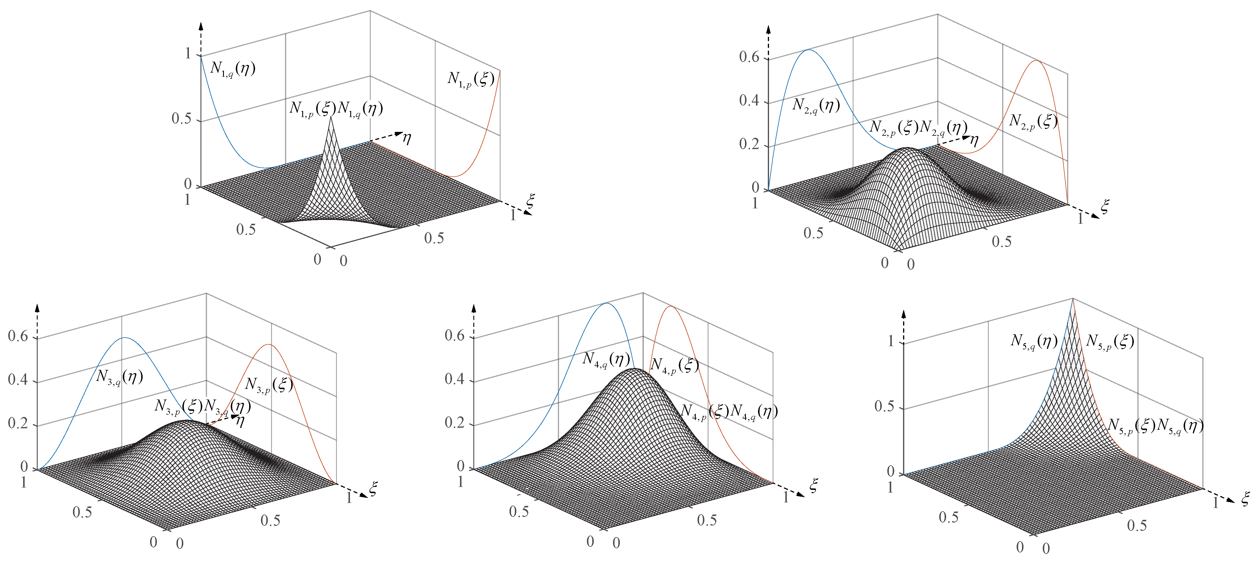
4. IGA-FEM Discretization of the Flexoelectric Fourth-Order Partial Differential Equation

In this study, the governing Equation (10) is discretized using B-splines basis functions. The Cox-de-Boor formula is used recursively to define the B-spline basis function [53,54,55,56,57], $N_{i,p}\left(\xi \right)$, and its expression is

$$\begin{array}{c}\hfill N_{i,0}\left(\xi \right)=\left\{\begin{array}{cc}1\hfill & \mathrm{if}{\xi }_i\le \xi <{\xi }_{i+1}\\ 0\hfill & \mathrm{otherwise}\end{array}\right.\end{array}$$

(31)

when $p=1,2,3,\dots \dots$

$$\begin{array}{c}\hfill N_{i,p}\left(\xi \right)=\frac{\xi -{\xi }_i}{{\xi }_{i+p}-{\xi }_i}{N}_{i,p-1}\left(\xi \right)+\frac{{\xi }_{i+p+1}-\xi }{{\xi }_{i+p+1}-{\xi }_{i+1}}{N}_{i+1,p-1}\left(\xi \right).\end{array}$$

(32)

Figure 1 depicts a schematic illustration of a specific B-spline multidimensional shape function, with all knot vectors being $\mathsf{\Xi }=\left. [\begin{array}{ccccccccc}0& 0& 0& 0& 0.5& 1& 1& 1& 1\end{array}\right]$. The multidimensional shape functions have orders p and q of three. It can be seen from Figure 1 that as long as the knot vectors $\mathsf{\Xi }$ and orders $p,q$ are specified, a very rich set of function types exists for the B-spline basis functions. This provides the continuity requirement for solving the flexoelectric governing equations. The linear algebraic discrete system equation of Equation (30) is written as

$$\begin{array}{c}\hfill \left. [\begin{array}{cc}{\mathrm{A}}_{uu}& {\mathrm{A}}_{u\phi }\\ {\mathrm{A}}_{\phi u}& {\mathrm{A}}_{\phi \phi }\end{array}\right]\left. [\begin{array}{c}\mathrm{u}\hfill \\ \mathsf{\Phi }\hfill \end{array}\right]=\left. [\begin{array}{c}{\mathrm{f}}_u\hfill \\ {\mathrm{f}}_{\phi }\hfill \end{array}\right]\end{array}$$

(33)

and

$$\begin{array}{cc}\hfill & {\mathrm{A}}_{uu}=\sum _e{\int }_{{\mathsf{\Omega }}_e}{\left({\mathrm{B}}_u\right)}^{\mathrm{T}}\mathrm{C}\left({\mathrm{B}}_u\right)\mathrm{d}{\mathsf{\Omega }}_e,\hfill \end{array}$$

(34)

$$\begin{array}{cc}\hfill & {\mathrm{A}}_{u\phi }=\sum _e{\int }_{{\mathsf{\Omega }}_e}[{\left({\mathrm{B}}_u\right)}^{\mathrm{T}}{\mathrm{e}}^{\mathrm{T}}\left({\mathrm{B}}_{\phi }\right)+{\left({\mathrm{H}}_u\right)}^{\mathrm{T}}{\mathbf{\mu }}^{\mathrm{T}}\left({\mathrm{B}}_{\phi }\right)]\mathrm{d}{\mathsf{\Omega }}_e,\hfill \end{array}$$

(35)

$$\begin{array}{cc}\hfill & {\mathrm{A}}_{\phi u}=\sum _e{\int }_{{\mathsf{\Omega }}_e}[{\left({\mathrm{B}}_{\phi }\right)}^{\mathrm{T}}\mathrm{e}\left({\mathrm{B}}_u\right)+{\left({\mathrm{B}}_{\phi }\right)}^{\mathrm{T}}\mathbf{\mu }\left({\mathrm{H}}_u\right)]\mathrm{d}{\mathsf{\Omega }}_e\hfill \end{array}$$

(36)

$$\begin{array}{cc}\hfill & {\mathrm{A}}_{\phi \phi }=-\sum _e{\int }_{{\mathsf{\Omega }}_e}{\left({\mathrm{B}}_{\phi }\right)}^{\mathrm{T}}\mathbf{\kappa }\left({\mathrm{B}}_{\phi }\right)\mathrm{d}{\mathsf{\Omega }}_e\hfill \end{array}$$

(37)

$$\begin{array}{cc}\hfill & {\mathrm{f}}_u=\sum _e{\int }_{{\mathsf{\Gamma }}_{t_e}}{{\mathrm{N}}_u}^{\mathrm{T}}{\mathrm{t}}_{\mathsf{\Gamma }}\mathrm{d}{\mathsf{\Gamma }}_{te}\hfill \end{array}$$

(38)

$$\begin{array}{cc}\hfill & {\mathrm{f}}_{\phi }=-\sum _e{\int }_{{\mathsf{\Gamma }}_{D_e}}{{\mathrm{N}}_{\phi }}^{\mathrm{T}}\omega \mathrm{d}{\mathsf{\Gamma }}_{De}.\hfill \end{array}$$

(39)

In Equations (34)–(39), the subscript e indicates the $e^{\mathrm{th}}$ finite element in ${\mathsf{\Omega }}_e$, ${\mathsf{\Gamma }}_{te}$, and ${\mathsf{\Gamma }}_{De}$, where $\mathsf{\Omega }={\cup }_e{\mathsf{\Omega }}_e$. The ${\mathrm{B}}_u$, ${\mathrm{B}}_{\phi }$, and ${\mathrm{H}}_u$ are listed below

$$\begin{array}{cc}\hfill & {\mathrm{B}}_u=\left. [\begin{array}{cccccccc}\frac{\partial N_1}{\partial x}& \frac{\partial N_2}{\partial x}& \cdots & \frac{\partial N_{ncp}}{\partial x}& 0& 0& 0& \cdots \\ 0& 0& \cdots & 0& \frac{\partial N_1}{\partial y}& \frac{\partial N_2}{\partial y}& \cdots & \frac{\partial N_{ncp}}{\partial y}\\ \frac{\partial N_1}{\partial y}& \frac{\partial N_2}{\partial y}& \cdots & \frac{\partial N_{ncp}}{\partial y}& \frac{\partial N_1}{\partial x}& \frac{\partial N_2}{\partial x}& \cdots & \frac{\partial N_{ncp}}{\partial y}\end{array}\right]\hfill \end{array}$$

(40)

$$\begin{array}{cc}\hfill & {\mathrm{B}}_{\phi }=\left. [\begin{array}{ccc}\frac{\partial N_1}{\partial x}& \cdots & \frac{\partial N_{ncp}}{\partial x}\\ \frac{\partial N_1}{\partial y}& \cdots & \frac{\partial N_{ncp}}{\partial y}\end{array}\right]\hfill \end{array}$$

(41)

$$\begin{array}{cc}\hfill & {\mathrm{H}}_u=\left. [\begin{array}{cccccccc}\frac{{\partial }^2{N}_1}{\partial x^2}& \frac{{\partial }^2{N}_2}{\partial x^2}& \cdots & \frac{{\partial }^2{N}_{ncp}}{\partial x^2}& 0& 0& \cdots & 0\\ 0& 0& \cdots & 0& \frac{{\partial }^2{N}_1}{\partial y\partial x}& \frac{{\partial }^2{N}_2}{\partial y\partial x}& \cdots & \frac{{\partial }^2{N}_{ncp}}{\partial y\partial x}\\ \frac{{\partial }^2{N}_1}{\partial y\partial x}& \frac{{\partial }^2{N}_2}{\partial y\partial x}& \cdots & \frac{{\partial }^2{N}_{ncp}}{\partial y\partial x}& \frac{{\partial }^2{N}_1}{\partial x^2}& \frac{{\partial }^2{N}_2}{\partial x^2}& \cdots & \frac{{\partial }^2{N}_{ncp}}{\partial x^2}\\ \frac{{\partial }^2{N}_1}{\partial x\partial y}& \frac{{\partial }^2{N}_2}{\partial x\partial y}& \cdots & \frac{{\partial }^2{N}_{ncp}}{\partial x\partial y}& 0& 0& \cdots & 0\\ 0& 0& \cdots & 0& \frac{{\partial }^2{N}_1}{\partial y^2}& \frac{{\partial }^2{N}_2}{\partial y^2}& \cdots & \frac{{\partial }^2{N}_{ncp}}{\partial y^2}\\ \frac{{\partial }^2{N}_1}{\partial y^2}& \frac{{\partial }^2{N}_2}{\partial y^2}& \cdots & \frac{{\partial }^2{N}_{ncp}}{\partial y^2}& \frac{{\partial }^2{N}_1}{\partial x\partial y}& \frac{{\partial }^2{N}_2}{\partial x\partial y}& \cdots & \frac{{\partial }^2{N}_{ncp}}{\partial x\partial y}.\end{array}\right]\hfill \end{array}$$

(42)

The matrix form of $\mathrm{C}$, $\mathbf{\kappa }$, $\mathrm{e}$, and $\mathbf{\mu }$ are

$$\begin{array}{cc}\hfill & \mathrm{C}=\left(\frac{Y}{(1+\nu )(1-2\nu )}\right)\left. [\begin{array}{ccc}1-\nu & \nu & 0\\ \nu & 1-\nu & 0\\ 0& 0& (\frac{1}{2}-\nu )\end{array}\right]\hfill \end{array}$$

(43)

$$\begin{array}{cc}\hfill & \mathbf{\kappa }=\left. [\begin{array}{cc}{\kappa }_{11}& 0\\ 0& {\kappa }_{22}\end{array}\right]\hfill \end{array}$$

(44)

$$\begin{array}{cc}\hfill & \mathrm{e}=\left. [\begin{array}{ccc}0& 0& e_{15}\\ e_{31}& e_{33}& 0\end{array}\right]\hfill \end{array}$$

(45)

$$\begin{array}{cc}\hfill & \mathbf{\mu }=\left. [\begin{array}{cccccc}{\mu }_{11}& {\mu }_{12}& 0& 0& 0& {\mu }_{44}\\ 0& 0& {\mu }_{44}& {\mu }_{12}& {\mu }_{11}& 0\end{array}\right]\hfill \end{array}$$

(46)

where the symbol Y stands for Young’s modulus and the symbol $\nu$ is the Poisson’s ratio.

5. Numerical Examples

In this section, we firstly use a benchmark example to verify the correctness of our analytical model. The confirmed IGA model is applied to the polynomial chaos expansion method to build the surrogate model. In the case of model verification, we assume that the model satisfies the plane strain hypothesis, as detailed in Equation (43).

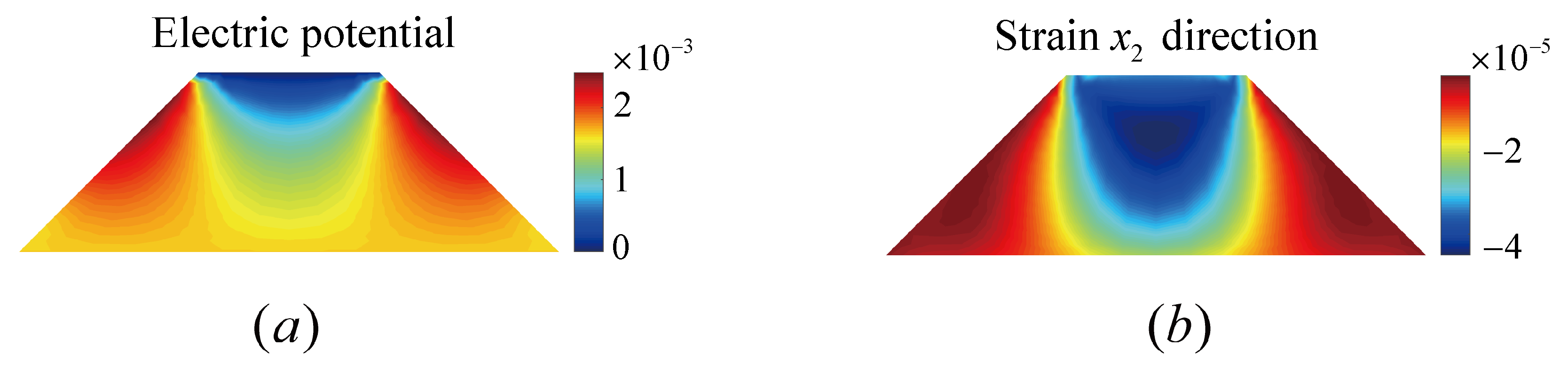
5.1. Model Validation

The truncated pyramid is the most commonly studied geometry in flexoelectric materials. The truncated pyramid model and the discretization meshing are shown in Figure 2. The upper edge is subjected to uniformly distributed forces of F magnitude, whilst the lower edge is immobile. The material parameters and detailed sizes of the model are shown in

Table 3. Material parameters for truncated pyramid.

Type	Symbol	Magnitude	Unit
Upper edge width	$a_1$	750	$\mathsf{\mu }\mathrm{m}$
Lower edge width	$a_2$	2250	$\mathsf{\mu }\mathrm{m}$
Thickness	h	750	$\mathsf{\mu }\mathrm{m}$
Distributed force	F	6	$N/\mathsf{\mu }\mathrm{m}$

. Here, we specify that the electric potential at the upper edge is 0. Here, we use the penalty function method to process the electric potential at the lower edge, resulting in an equipotential boundary condition. On this benchmark case, we obtain the electric potential and strain distributions depicted in Figure 3. The electric potential and strain distributions are essentially comparable to those observed in [10].

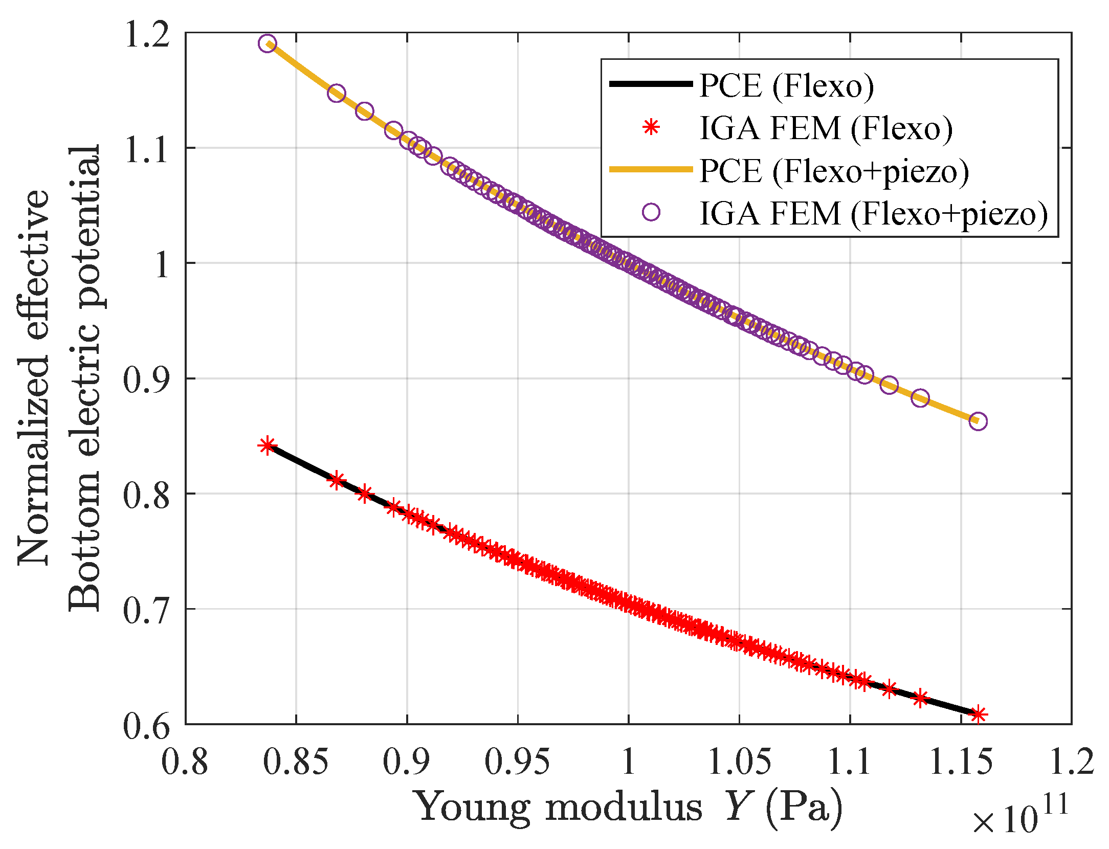
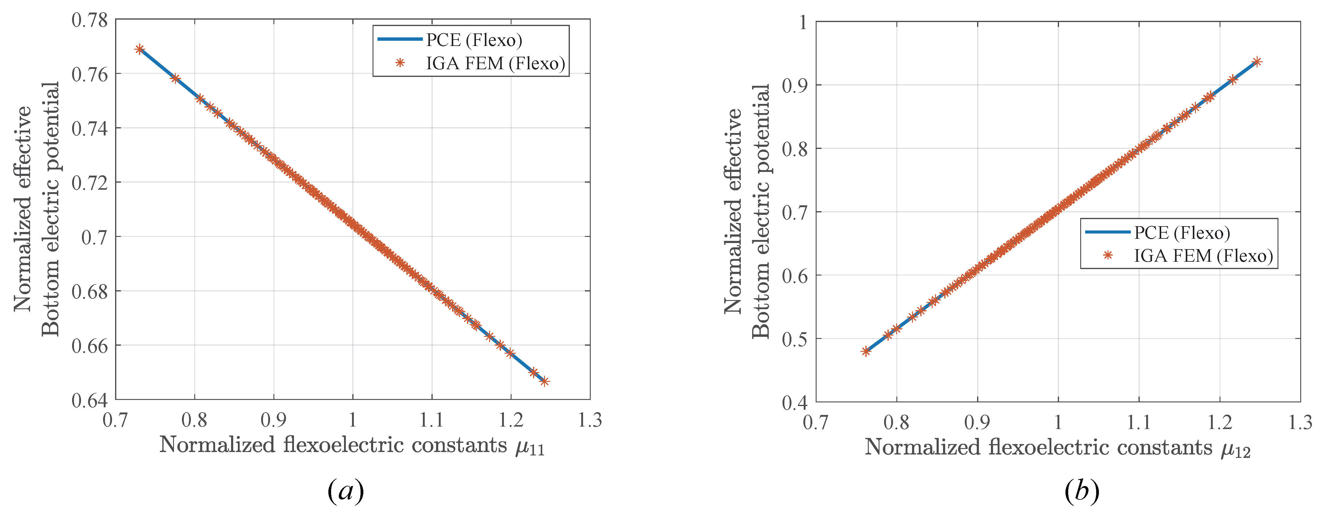
5.2. Verification of Surrogate Models for Mechanical Properties of Flexoelectric Materials

In this section, we will employ the truncated pyramid model from Section 5.1 to construct a surrogate model of the mechanical properties of materials with significant strain gradients. Owing to the equipotential boundary condition at the lower edge, we use the electric potential at the lower edge as the response result required to construct the surrogate model. The random input parameters are chosen as Young’s modulus, uniformly distributed force and two flexoelectric constants, respectively. The range of values and statistical characteristics of the random input parameters are listed in

Table 4. Range of values and the statistical properties of the random input parameters.

Random Input Parameters	Expected Values $\mathcal{E}$	Coefficient of Variation $\mathit{\gamma }$	The Input Parameters’ Limitations:
			[Lower, Upper]
Young’s modulus Y	1 × 10${}^{11}$	0.06	[8.20 × 10${}^{10}$, 1.18 × 10${}^{11}$]
Uniformly distributed force F	6 × 10${}^6$	0.06	[4.92 × 10${}^6$, 7.08 × 10${}^6$]
Flexoelectric constant ${\mu }_{11}$/${\mu }_{12}$	1 × 10${}^{-6}$	0.1	[7.00 × 10${}^{-7}$, 1.30 × 10${}^{-6}$]

.

The compared results of PCE and IGA-FEM of the electric potential generated by the material under excitation are shown in Figure 4, where the random input parameter is Young’s modulus. From Figure 4, it can be seen that the IGA-FEM and PCE results are consistent, confirming the algorithm’s validity. It is also shown that the magnitude of the elastic stiffness affects the results of the electric potential generated by the excitation of piezoelectric and non-piezoelectric materials, which is due to the magnitude of the elastic modulus affecting the elastic stiffness of the structure.

Figure 5 shows the compared results of PCE and IGA-FEM of the electric potential generated by the excitation of the material when a uniformly distributed force is utilized as a random parameter. The graphic shows that when the normalized uniform distribution force grows, so does the normalized outcome of electric potential. The electrical potential generated by a piezoelectric material under excitation is larger than that of a non-piezoelectric material.

Since the flexoelectric effect is weak in piezoelectric materials, the PCE model of piezoelectric materials whose flexoelectric constants are random parameters is not considered. The compared results of PCE and IGA-FEM of the material subjected to excitation to generate electric potential are shown in Figure 6, where the random input parameters are the flexoelectric constants ${\mu }_{11}$ and ${\mu }_{12}$. As seen in Figure 6, as the normalized flexoelectric constant increases, the normalized electric potential values exhibit an opposite trend. Through PCE, a surrogate modeling of mechanical properties can be established under small sample conditions and the calculation accuracy can be guaranteed. This is an advantage that distinguishes it from other uncertainty quantification methods such as MCs.

6. Conclusions

In this work, a polynomial chaos expansion based on the isogeometric FEM is used to study the mechanical properties of flexoelectric materials, the key points are as follows:

1.

The B-spline shape functions satisfying the continuity requirement are employed to discretize the governing equations.

2.

The IGA-FEM reduces the need for repeated meshing in uncertainty quantification while maintaining geometric accuracy.

3.

The truncated pyramid model was chosen as the object of study to obtain the mechanical properties of the flexoelecteric material.

The present method is not without limitations. It is difficult to efficiently compute the mechanical response of a material when the dimension of the input random variable is multidimensional. Therefore, the development of efficient methods for the analysis of mechanical properties of multidimensional random variables is the focus of our future work.

References

1. Mashkevich, V.; Tolpygo, K. Electrical, optical and elastic properties of diamond type crystals. Sov. Phys. JETP 1957, 5, 435–439. [Google Scholar]
2. Ahmadpoor, F.; Sharma, P. Flexoelectricity in two-dimensional crystalline and biological membranes. Nanoscale 2015, 7, 16555–16570. [Google Scholar] [CrossRef]
3. Ahmadpoor, F.; Lahmer, T.; Zhuang, X.; Zi, G.; Rabczuk, T. Detection of material interfaces using a regularized level set method in piezoelectric structures. Inverse Probl. Sci. Eng. 2016, 24, 153–176. [Google Scholar] [CrossRef]
4. Yudin, P.; Tagantsev, A. Fundamentals of flexoelectricity in solids. Nanotechnology 2013, 24, 432001. [Google Scholar] [CrossRef]
5. Nguyen, T.D.; Mao, S.; Yeh, Y.W.; Purohit, P.K.; McAlpine, M.C. Nanoscale flexoelectricity. Adv. Mater. 2013, 25, 946–974. [Google Scholar] [CrossRef] [PubMed]
6. Zubko, P.; Catalan, G.; Tagantsev, A.K. Flexoelectric effect in solids. Annu. Rev. Mater. Res. 2013, 43, 387–421. [Google Scholar] [CrossRef]
7. Vinyas, M.; Nischith, G.; Loja, M.A.R.; Ebrahimi, F.; Duc, N.D. Numerical analysis of the vibration response of skew magneto-electro-elastic plates based on the higher-order shear deformation theory. Compos. Struct. 2019, 214, 132–142. [Google Scholar] [CrossRef]
8. Zhao, Q.; Liu, Y.; Wang, L.; Yang, H.; Cao, D. Design method for piezoelectric cantilever beam structure under low frequency condition. Int. J. Pavement Res. Technol. 2018, 11, 153–159. [Google Scholar] [CrossRef]
9. Majdoub, M.S.; Sharma, P.; Cagin, T. Enhanced size-dependent piezoelectricity and elasticity in nanostructures due to the flexoelectric effect. Phys. Rev. B 2008, 77, 125424. [Google Scholar] [CrossRef]
10. Abdollahi, A.; Peco, C.; Millán, D.; Arroyo, M.; Arias, I. Computational evaluation of the flexoelectric effect in dielectric solids. J. Appl. Phys. 2014, 116, 093502. [Google Scholar] [CrossRef]
11. Blatman, G. Adaptive Sparse Polynomial Chaos Expansions for Uncertainty Propagation and Sensitivity Analysis. Ph.D. Thesis, Blaise Pascal University, Aubiere, France, 2009. [Google Scholar]
12. Kumar, Y.A.; Mani, G.; Pallavolu, M.R.; Sangaraju, S.; Reddy, N.R.; Selvaraj, M.; Alfakeer, M.; Bahajjaj, A.A.A.; Ouladsmane, M.; Rao, S.S.R.; et al. Facile synthesis of efficient construction of tungsten disulfide/iron cobaltite nanocomposite grown on nickel foam as a battery-type energy material for electrochemical supercapacitors with superior performance. J. Colloid Interface Sci. 2022, 609, 434–446. [Google Scholar] [CrossRef]
13. Moniruzzaman, M.; Kumar, Y.A.; Pallavolu, M.R.; Arbi, H.M.; Alzahmi, S.; Obaidat, I. Two-dimensional core-shell structure of cobalt-doped@MnO2 nanosheets grown on nickel foam as a binder-free battery-type electrode for supercapacitor application. Nanomaterials 2022, 12, 3187. [Google Scholar] [CrossRef]
14. Pallavolu, M.R.; Kumar, Y.A.; Reddy, N.M.; Dhananjaya, M.; Al-Asbahi, B.A.; Sreedhar, A.; Joo, S.W. Design and synthesis of highly efficient Nitrogen-doped carbon nano-onions for asymmetric supercapacitors. J. Alloy. Compd. 2022, 918, 165609. [Google Scholar] [CrossRef]
15. Hurtado, J.; Barbat, A. Monte Carlo techniques in computational stochastic mechanics. Arch. Comput. Methods Eng. 1998, 5, 3–29. [Google Scholar] [CrossRef]
16. Honda, R. Stochastic BEM with spectral approach in elastostatic and elastodynamic problems with geometrical uncertainty. Eng. Anal. Bound. Elem. 2005, 29, 415–427. [Google Scholar] [CrossRef]
17. Liu, W.K.; Belytschko, T.; Mani, A. Random field finite elements. Int. J. Numer. Methods Eng. 1986, 23, 1831–1845. [Google Scholar] [CrossRef]
18. Kamiński, M. Stochastic perturbation approach to engineering structure vibrations by the finite difference method. J. Sound Vib. 2002, 251, 651–670. [Google Scholar] [CrossRef]
19. Kamiński, M. On generalized stochastic perturbation-based finite element method. Commun. Numer. Methods Eng. 2006, 22, 23–31. [Google Scholar] [CrossRef]
20. Zhang, B.Y.; Ni, Y.Q. A hybrid sequential sampling strategy for sparse polynomial chaos expansion based on compressive sampling and Bayesian experimental design. Comput. Methods Appl. Mech. Eng. 2021, 386, 114130. [Google Scholar] [CrossRef]
21. Kersaudy, P.; Sudret, B.; Varsier, N.; Picon, O.; Wiart, J. A new surrogate modeling technique combining Kriging and polynomial chaos expansions–Application to uncertainty analysis in computational dosimetry. J. Comput. Phys. 2015, 286, 103–117. [Google Scholar] [CrossRef]
22. Novak, L.; Novak, D. Polynomial chaos expansion for surrogate modelling: Theory and software. Beton-Stahlbetonbau 2018, 113, 27–32. [Google Scholar] [CrossRef]
23. Wan, H.P.; Ren, W.X.; Todd, M.D. Arbitrary polynomial chaos expansion method for uncertainty quantification and global sensitivity analysis in structural dynamics. Mech. Syst. Signal Process. 2020, 142, 106732. [Google Scholar] [CrossRef]
24. Rajabi, M.M.; Ataie-Ashtiani, B.; Simmons, C.T. Polynomial chaos expansions for uncertainty propagation and moment independent sensitivity analysis of seawater intrusion simulations. J. Hydrol. 2015, 520, 101–122. [Google Scholar] [CrossRef]
25. Guo, X.; Dias, D.; Claudio, C.; Laurent, P.; Pierre, B. Reliability analysis of embankment dam sliding stability using the sparse polynomial chaos expansion. Eng. Struct. 2018, 174, 295–307. [Google Scholar] [CrossRef]
26. Hariri, A.; Mohammad, A.; Claudio, C.; Sudret, B. Polynomial chaos expansion for uncertainty quantification of dam engineering problems. Eng. Struct. 2020, 203, 109631. [Google Scholar] [CrossRef]
27. Matthies, H.G.; Keese, A. Galerkin methods for linear and nonlinear elliptic stochastic partial differential equations. Comput. Methods Appl. Mech. Eng. 2005, 194, 1295–1331. [Google Scholar] [CrossRef]
28. Cao, G.; Yu, B.; Chen, L.; Yao, W. Isogeometric dual reciprocity BEM for solving non-Fourier transient heat transfer problems in FGMs with uncertainty analysis. Int. J. Heat Mass Transf. 2023, 203, 123783. [Google Scholar] [CrossRef]
29. Le Maître, O.; Knio, O.M. Spectral Methods for Uncertainty Quantification with Applications to Computational Fluid Dynamics; Springer: Dordrecht, The Netherlands, 2010. [Google Scholar] [CrossRef]
30. Blatman, G.; Sudret, B. Sparse polynomial chaos expansions and adaptive stochastic finite elements using a regression approach. Comptes Rendus Mec. 2008, 336, 518–523. [Google Scholar] [CrossRef]
31. Palar, P.S.; Tsuchiya, T.; Parks, G.T. Multi-fidelity non-intrusive polynomial chaos based on regression. Comput. Methods Appl. Mech. Eng. 2016, 305, 579–606. [Google Scholar] [CrossRef]
32. Zhou, Y.; Lu, Z.; Cheng, K.; Shi, Y. An expanded sparse Bayesian learning method for polynomial chaos expansion. Mech. Syst. Signal Process. 2019, 128, 153–171. [Google Scholar] [CrossRef]
33. Hughes, T.J.; Cottrell, J.A.; Bazilevs, Y. Isogeometric analysis: CAD, finite elements, NURBS, exact geometry and mesh refinement. Comput. Methods Appl. Mech. Eng. 2005, 194, 4135–4195. [Google Scholar] [CrossRef]
34. Ghasemi, H.; Park, H.S.; Alajlan, N.; Rabczuk, T. A computational framework for design and optimization of flexoelectric materials. Int. J. Comput. Methods 2020, 17, 1850097. [Google Scholar] [CrossRef]
35. Li, H.; Zhao, J.; Guo, X.; Cheng, Y.; Xu, Y.; Yuan, X. Sensitivity analysis of flexoelectric materials surrogate model based on the isogeometric finite element method. Front. Phys. 2022, 10, 1343. [Google Scholar] [CrossRef]
36. Schillinger, D.; Dede, L.; Scott, M.A.; Evans, J.A.; Borden, M.J.; Rank, E.; Hughes, T.J. An isogeometric design-through-analysis methodology based on adaptive hierarchical refinement of NURBS, immersed boundary methods, and T-spline CAD surfaces. Comput. Methods Appl. Mech. Eng. 2012, 249, 116–150. [Google Scholar] [CrossRef]
37. Chen, L.; Lian, H.; Xu, Y.; Li, S.; Liu, Z.; Atroshchenko, E.; Kerfriden, P. Generalized isogeometric boundary element method for uncertainty analysis of time-harmonic wave propagation in infinite domains. Appl. Math. Model. 2023, 114, 360–378. [Google Scholar] [CrossRef]
38. Evans, J.A.; Hughes, T.J. Isogeometric divergence-conforming B-splines for the unsteady Navier–Stokes equations. J. Comput. Phys. 2013, 241, 141–167. [Google Scholar] [CrossRef]
39. Chen, L.; Liu, C.; Zhao, W.; Liu, L. An isogeometric approach of two dimensional acoustic design sensitivity analysis and topology optimization analysis for absorbing material distribution. Comput. Methods Appl. Mech. Eng. 2018, 336, 507–532. [Google Scholar] [CrossRef]
40. Chen, L.; Lian, H.; Liu, Z.; Chen, H.; Atroshchenko, E.; Bordas, S. Structural shape optimization of three dimensional acoustic problems with isogeometric boundary element methods. Comput. Methods Appl. Mech. Eng. 2019, 355, 926–951. [Google Scholar] [CrossRef]
41. Chen, L.; Cheng, R.; Li, S.; Lian, H.; Zheng, C.; Bordas, S.P. A sample-efficient deep learning method for multivariate uncertainty qualification of acoustic–vibration interaction problems. Comput. Methods Appl. Mech. Eng. 2022, 393, 114784. [Google Scholar] [CrossRef]
42. Chen, L.; Lu, C.; Lian, H.; Liu, Z.; Zhao, W.; Li, S.; Chen, H.; Bordas, S.P. Acoustic topology optimization of sound absorbing materials directly from subdivision surfaces with isogeometric boundary element methods. Comput. Methods Appl. Mech. Eng. 2020, 362, 112806. [Google Scholar] [CrossRef]
43. Lu, C.; Chen, L.; Luo, J.; Chen, H. Acoustic shape optimization based on isogeometric boundary element method with subdivision surfaces. Eng. Anal. Bound. Elem. 2023, 146, 951–965. [Google Scholar] [CrossRef]
44. Jiang, F.; Chen, L.; Wang, J.; Miao, X.; Chen, H. Topology optimization of multimaterial distribution based on isogeometric boundary element and piecewise constant level set method. Comput. Methods Appl. Mech. Eng. 2022, 390, 114484. [Google Scholar] [CrossRef]
45. Jiang, F.; Zhao, W.; Chen, L.; Zheng, C.; Chen, H. Combined shape and topology optimization for sound barrier by using the isogeometric boundary element method. Eng. Anal. Bound. Elem. 2021, 124, 124–136. [Google Scholar] [CrossRef]
46. Liu, C.; Chen, L.; Zhao, W.; Chen, H. Shape optimization of sound barrier using an isogeometric fast multipole boundary element method in two dimensions. Eng. Anal. Bound. Elem. 2017, 85, 142–157. [Google Scholar] [CrossRef]
47. Jahanbin, R.; Rahman, S. Stochastic isogeometric analysis in linear elasticity. Comput. Methods Appl. Mech. Eng. 2020, 364, 112928. [Google Scholar] [CrossRef]
48. Liu, Z.; Yang, M.; Cheng, J.; Tan, J. A new stochastic isogeometric analysis method based on reduced basis vectors for engineering structures with random field uncertainties. Appl. Math. Model. 2021, 89, 966–990. [Google Scholar] [CrossRef]
49. Xiu, D.; Karniadakis, G.E. The Wiener–Askey polynomial chaos for stochastic differential equations. SIAM J. Sci. Comput. 2002, 24, 619–644. [Google Scholar] [CrossRef]
50. Cao, L.; Liu, J.; Jiang, C.; L, G. Optimal sparse polynomial chaos expansion for arbitrary probability distribution and its application on global sensitivity analysis. Comput. Methods Appl. Mech. Eng. 2022, 399, 115368. [Google Scholar] [CrossRef]
51. Hauseux, P.; Hale, J.S.; Bordas, S.P. Accelerating Monte Carlo estimation with derivatives of high-level finite element models. Comput. Methods Appl. Mech. Eng. 2017, 318, 917–936. [Google Scholar] [CrossRef]
52. Ghasemi, H.; Park, H.S.; Rabczuk, T. A level-set based IGA formulation for topology optimization of flexoelectric materials. Comput. Methods Appl. Mech. Eng. 2017, 313, 239–258. [Google Scholar] [CrossRef]
53. Chen, L.; Lian, H.; Natarajan, S.; Zhao, W.; Chen, X.; Bordas, S.P.A. Multi-frequency acoustic topology optimization of sound-absorption materials with isogeometric boundary element methods accelerated by frequency-decoupling and model order reduction techniques. Comput. Methods Appl. Mech. Eng. 2022, 395, 114997. [Google Scholar] [CrossRef]
54. Chen, L.; Lian, H.; Liu, Z.; Gong, Y.; Zheng, C.J.; Bordas, S.P.A. Bi-material topology optimization for fully coupled structural-acoustic systems with isogeometric FEM–BEM. Eng. Anal. Bound. Elem. 2022, 135, 182–195. [Google Scholar] [CrossRef]
55. Chen, L.; Wang, Z.; Peng, X.; Yang, J.; Wu, P.; Lian, H. Modeling pressurized fracture propagation with the isogeometric BEM. Geomech. Geophys. Geo-Energy Geo-Resour. 2021, 7, 51. [Google Scholar] [CrossRef]
56. Chen, L.; Zhang, Y.; Lian, H.; Atroshchenko, E.; Ding, C.; Bordas, S.P.A. Seamless integration of computer-aided geometric modeling and acoustic simulation: Isogeometric boundary element methods based on Catmull-Clark subdivision surfaces. Adv. Eng. Softw. 2020, 149, 102879. [Google Scholar] [CrossRef]
57. Chen, L.; Li, H.; Guo, Y.; Chen, P.; Atroshchenko, E.; Lian, H. Uncertainty quantification of mechanical property of piezoelectric materials based on isogeometric stochastic FEM with generalized nth-order perturbation. Eng. Comput. 2023, 1–21. [Google Scholar] [CrossRef]
Figure 1. Schematic diagram of the B-spline shape functions with a specific knot vectors.
Sustainability 15 03417 g001
Figure 2. Truncated pyramid model where the upper edge is subjected to uniformly distributed force F (a), and the discretization meshing (b).
Sustainability 15 03417 g002
Figure 3. The distribution of overall electric potential φ (a), and the distribution of strain in the x 2 direction ( S 22 ) (b).
Sustainability 15 03417 g003
Figure 4. Comparison findings of IGA-FEM and PCE with Young’s modulus as a random parameter.
Sustainability 15 03417 g004
Figure 5. Comparison findings of IGA-FEM and PCE with uniformly distributed force as a random parameter.
Sustainability 15 03417 g005
Figure 6. Comparison findings of IGA-FEM and PCE. (a) The flexoelectric constant μ 11 is a random parameter. (b) The flexoelectric constant μ 12 is a random parameter.
Sustainability 15 03417 g006