Abstract
Groundwater storage is influenced by many geo-environmental factors. Most of these factors are prepared in the form of categorical data. The present study utilized raster satellite data instead of categorical data and a Random Forest machine learning model to identify groundwater potential zones at the downstream parts of Wadi Yalamlam, western Saudi Arabia. Eighteen groundwater-influenced variables are prepared in continuous raster format from ASTER GDEM, TRMM, and SPOT-5 satellite data. The Random Forest (RF) model is trained using (70%) of the target variable and validated using the rest (30%). The accuracy, sensitivity, and F1-score are all generated to evaluate the model performance. SPOT band 3, band 4, and the rainfall variables are the most important for groundwater potential mapping contributing 11%, 7%, and 8% during the prediction stage. The GDEM elevation variable contributed 6% and the slope variable scored 1%. The main conclusions of the study are: (1) The RF machine learning algorithm successfully identified three groundwater potential zones with an accuracy of 96%. (2) The high, moderate, and low potential groundwater zones covered 11.5%, 59.9%, and 28.6% of the study area respectively. (3) Majority of high and moderate zones lie within the pumping rate range between 10 and 20 m3/day. (4) The approach developed in this study can be applied to any other wadis having the same conditions to help authorities and decision-makers in planning and development projects.
1. Introduction
Freshwater represents a challenge for many countries in the Middle East. This is due to scarcity of rainfall and high demand for water to meet domestic, agricultural, and developmental needs. Saudi Arabia is one of the countries in the Middle East that endues an extremely hot and dry climate. It depends on desalinated seawater for domestic use while groundwater, renewable and non-renewable, is depended on to cover other demands. Rapid economic development and population growth increase the stress on freshwater resources. The freshwater demands of the Makkah Al-Mukarramah province, western Saudi Arabia, increase continuously, especially during the Omra and Pilgrimage seasons due to the expansion of the holly mosques capacities and the development of mega-projects [1].
Most of the water consumed for domestic use in the Makkah Al-Mukarramah province is desalinated seawater, while renewable groundwater is used for agricultural activities. Wadi Yalamlam is one of the major wadis close to Makkah Al-Mukarramah city that contributes to satisfying the village’s freshwater needs and the agricultural demands of the city’s vicinity. Groundwater resources in Wadi Yalamlam (Figure 1) are investigated by many authors such as [2,3,4,5,6,7]. All previous investigations of groundwater resources in Wadi Yalamlam mentioned above used conventional methods. In [1], the groundwater resources in Wadi Yalamlam were evaluated using hydrological, hydrochemical, and geophysical techniques. The study indicated the possibility of drilling 14 water wells for producing a renewable amount of 7500 m3/day to supply the Makkah province. In [7], the groundwater quality in the Wadi Yalamlam basin was evaluated using the irrigation water quality index (IWQI) and drinking water quality index (DWQI).
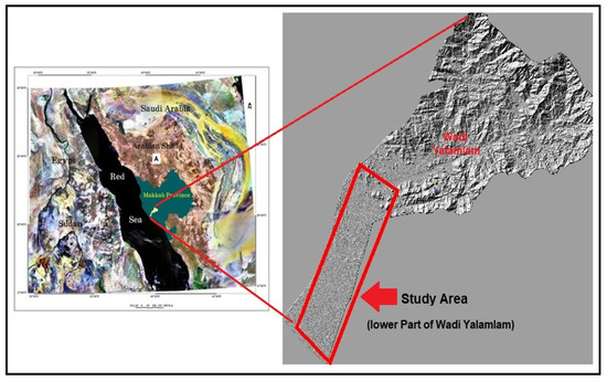
Figure 1.
Location of the study area.
Groundwater potential mapping is an important issue in groundwater management and sustainability. Remote sensing data and GIS techniques are important in generating groundwater potential maps [5,8,9,10,11,12]. The authors of [12] delineated groundwater potential zones in the central Eastern Desert, Egypt using the applications of remote sensing and GIS techniques. The authors of [6] developed an integrated approach that utilized remote sensing and airborne magnetic data to identify the Quaternary aquifers impounded by dykes in the study area. They explained the dykes-lineaments relationship and their effects on groundwater storage. The authors of [5] presented a groundwater potential map for the Wadi Yalamlam basin, using the weights of evidence GIS model. They concluded that downstream parts of Wadi Yalamlam are the most promising for groundwater potentiality.
The subject of generating groundwater potential zones (GWPM) using machine learning (ML) algorithms has been dealt with by many authors such as [13,14,15,16,17,18,19,20,21,22]. The most frequent machine learning models used to generate GWPM are Random Forest, support vector machine, multivariate adaptive regression splines, K-nearest neighbor, classification and regression tree, and the artificial neural network model. The authors of [19] evaluated different machine learning algorithms to groundwater potential mapping. They utilized fifteen geo-environmental factors as independent variables (categorical and continuous). Results revealed that RF has the best performance (90%). The authors of [21] generated a groundwater potential map in the Center East Desert, Egypt, using a random forest model. They utilized fifteen effective features influencing groundwater potentiality. The model performance is evaluated using accuracy (97%) and sensitivity (92%). The authors of [22] utilized four methods of machine learning, deep learning, ensemble learning, and automated machine learning (AutoML) to identify groundwater potential zones in Hubei Province, China. Results revealed that automated machine learning method learning (AutoML) has high performance with accuracy 88%. The random forest (RF) model is the most successful classifier used in the groundwater potential mapping due to many reasons mentioned by [21]. The Random Forest (RF) model requires target and explanatory variables. The target variable is represented by groundwater field measurements whereas the explanatory variables contain features related to groundwater storage. Wadi Yalamlam was chosen to be under investigation to identify groundwater potential zones for two reasons: the availability of the field measurements of groundwater levels, and the importance of this wadi (supplies the pilgrims’ station, which is a passing station for pilgrims from the south part of Arabian Peninsula and East Africa) for Yalamlam Miqat. The present study aims to identify the groundwater potential zones at downstream parts of Wadi Yalamlam using Random Forest (RF) machine learning algorithm. This study presents a new approach that utilizes continuous SPOT-5 satellite data as explanatory variables. The idea is to utilize raw continuous raster data instead of the categorical classified data to overcome the bias that arises due to differences in the variable’s data range. All explanatory variables extracted from the processed satellite data are prepared in continuous raster format. No categorical variables are used as explanatory variables. The only categorical data used in this study is the target variable which is classified into three categories. Previous studies that utilized both raster and categorical data as explanatory variables performed a pre-processing scaling step before running the ML models [23,24,25,26].
2. Study Area and the Hydrogeological Setting
The study area (Figure 1) covered the downstream parts of Wadi Yalamlam. It is bounded by longitudes 39°47′43″ E 40°01′27″ E and latitudes 20°26′42″ N to 20°50′14″ N. Figure 2 represents a 3D view of a Rapideye image draped over ASTER GDEM elevation data. The subsurface information of the cross-section was obtained from well/farms distributed over the study area. Elevations in the study area vary between 600 m and 25 m (a.s.l.). Wadi Yalamlam has N–S to NNE-SSW directions and crosscuts the highly altered and fractured granitic gneiss and metabasalts. From a geomorphologic point of view, the study area is covered by: (1) basement rocks covered the northeastern part of the study area with the highest elevation reaching 600 m (a.s.l.) at Gabal Al Ghamdiyah, (2) a coastal plain area located at the south part of the study area facing the red sea coast with an average elevation of 25 m (a.s.l.), and (3) a hilly dyke area that lies in the middle of the study area.
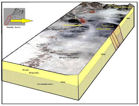
Figure 2.
3D perspective view of RapidEye image draped over GDEM elevation data for the study area. The subsurface information was collected from wells distributed along the study area.
Most of the study area is covered by basement rocks and Quaternary deposits (alluvial and aeolian). The principal aquifer in the study area is the Quaternary wadi deposits. Depths to the groundwater vary from 8 m to 30 m. The general flow direction is toward the southwest [5]. As shown in Figure 2, the middle part is covered mainly by dyke swarms separating the northern part of the study area from the southern part. These dykes separate the shallow wells (8 m) around Sheikh Said farm from the relatively deep wells (16 m) in the south part of the study area. Depths to groundwater in the dyke region range between 15 and 30 m. Depths to groundwater measurements are collected from wells during the field visits and are used as part of the target variable.
3. Materials and Methods
Figure 3 shows the various steps used to identify and map the groundwater potential zones in the study area. SPOT 5, TRMM, and ASTER GDEM raster data are processed to produce eighteen continuous raster features used as explanatory variables. The idea of performing the RF model using continuous raster data (raw and processed) instead of categorical classified data is to overcome the bias that arises due to differences in the variable’s data range. Image subsets from the original SPOT multispectral images were prepared and used as inputs in the RF model. Band ratio, PCA, and NDVI are the main image processing techniques used to generate the different datasets of the explanatory variables. ASTER GDEM elevation data are used to prepare the slope image. TRMM rainfall data are used in the model. A dependent variable (168 points) is collected and used in the RF model. These points are composed of depths to groundwater measurements and non-potential sites. It was split into 70% used for training the model and 30% for validation. The accuracy, F1_score, and sensitivity are all generated to test the model performance. The resulting groundwater potential map was evaluated using available pumping rate data. A Random Forest model was performed using the ArcGIS Pro package.
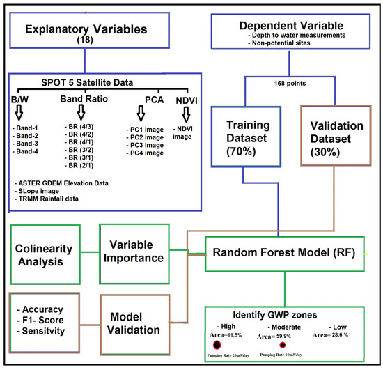
Figure 3.
Methodology flowchart for identifying GWP zones using the RF model.
3.1. Explanatory and Dependent Variables
Figure 4 shows the target variable that contains depths of groundwater collected from wells during the field visits. It includes the non-groundwater potential sites. The target variable is classified into high (1), moderate (2), and low/non-groundwater potential (0). The authors of [5] generated a pumping rate map using data collected by [1]. It shows that the majority of the study area lies within the low pumping rate category (10–20 m3/day).
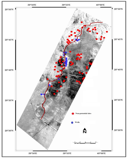
Figure 4.
Points of target variable.
The recharge of the groundwater is influenced by climatic, topographic, and geologic factors such as rainfall, elevation, slope, geomorphology, lithology, land use/landcover, lineaments, faults, soil type, vegetation index, topographic wetness index, water table depth, and groundwater quality [5,23,24]. Band ratio, PCA, and NDVI are used to generate different datasets used in the model. Band ratio is an important technique used for lithologic discrimination [25,26,27]. It is generated by dividing the reflectance value of each pixel in one band by the reflectance value of the same pixel in another band [28]. Figure 5a–f show the results of the band ratio technique. The 4/3, 4/2, and 4/1 band ratio images discriminate the basement rocks (baish basalts and granites) in which they have white and dark to dark grey image signatures, respectively. Quaternary deposits have grey to light grey image signatures and discriminated into alluvial (grey) and aeolian deposits on 3/2, 3/1, and 2/1 images. The dyke zone has a dark image signature. Principal Component Analysis (PCA) produced a set of principal components ordered in terms of decreasing the information content. Figure 6a–d show the results of the PCA technique. The normalized difference vegetation index (NDVI) is generated to quantify the green vegetation (Figure 6e). It is calculated using the following equation: NDVI = (B3−B2)/(B3+B2), where B2 and B3 represent SPOT band 2 and 3 covering Red: 610–680 nm and Near IR: 780–890 nm wavelength regions. ASTER GDEM elevation data (Figure 6f) is generated using stereo-pair images (bands 3N and 3B). The study area is characterized by low elevation values except for the northern areas. Flat areas with low slope values and high infiltration are capable of holding rainfall and causing recharge of the groundwater. The slope image (Figure 6g) is generated using GDEM elevation data. Figure 6h shows the rainfall map generated using TRMM rainfall data collected between 2000 and 2014. The rainfall distribution is strongly affected by the topography of the study area. Drainage density is excluded from the dataset due to its negligible effects on the groundwater recharge in the study area. Table 1 demonstrates the data sets used in this study. They include: (1) Black and White (B/W) raw SPOT imageries (bands 1, 2, 3, and 4), (2) Band ratio images (BR) 4/3, 4/2, 4/1, 3/2, 3/1, and 2/1, (3) Principal Component images (PC1, PC2, PC3, and PC4) (4) NDVI vegetation index image, (5) TRMM rainfall image, (6) GDEM elevation and slope images.
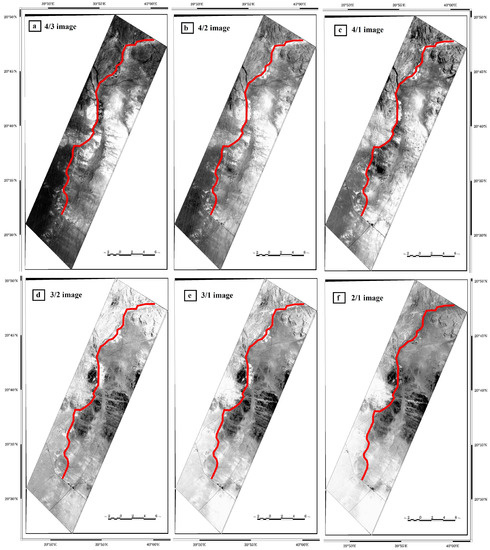
Figure 5.
Explanatory variables (band ratio images).
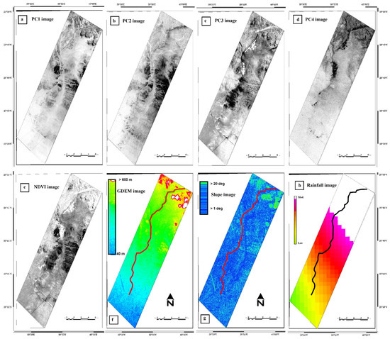
Figure 6.
Explanatory variables (cont.): (a) PC1, (b) PC2, (c) PC3, (d) PC4, (e) NDVI image, (f) GDEM elevation data, (g) slope image, and (h) TRMM rainfall image.

Table 1.
Data sets used as explanatory variables in the present study.
3.2. Random Forest Algorithm and Model Performance
Random Forest is a machine learning algorithm used for regression and classification tasks. It is used to identify GWP zones at the downstream part of Wadi Yalamlam. A Random Forest algorithm works by creating multiple decision trees, each of which used a random subset of the explanatory variables, and then averaging their results (Figure 7). Decision trees make predictions by looking at the datasets and determining which category they belong to. The RF model allows the user to build optimal decision trees based on the aggregation of multiple iterative trees built from randomly selected samples of the training step [29]. Several authors demonstrated its ability to rank the important variables during the training and prediction stages [30,31]. The two main parameters required for the RF model are the number of trees and the number of variables. In the present work, the first parameter is set to default (100). In this study, the accuracy, sensitivity, and F1_score are all generated to evaluate the model performance.
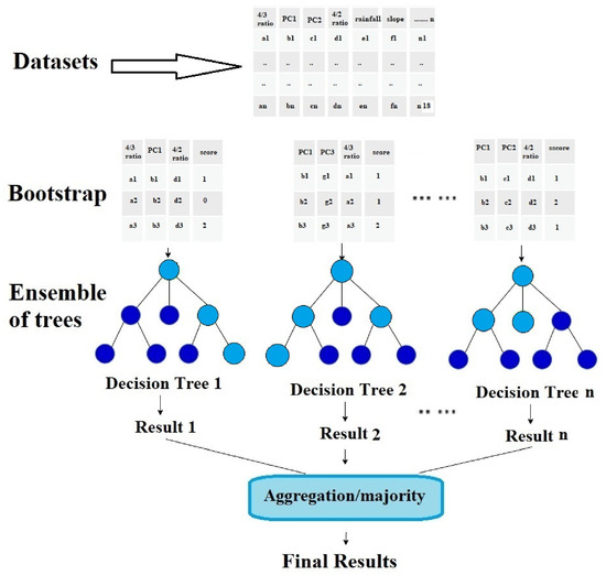
Figure 7.
The Random Forest model.
4. Results
4.1. Collinearity Analysis
Collinearity is a statistical technique represents a linear relationship between two independent variables. It is performed before the RF model implementation. It can influence the performance of the model by adding noise to the outcomes [32]. Figure 8 shows the linear relationship between some selected variables of the study area. It shows no significant correlation between the explanatory variables except the linear positive correlation between: (1) band ratios 4/3 & 4/2 with R2 = 0.59; (2) band ratios 3/1 & 3/2 with R2 = 0.92; and (3) band ratios 3/1 & 2/1 with R2 = 0.8. Ref. [33] concluded that the R2 values between 0.4 and 0.85 are acceptable levels for correlation between two variables.
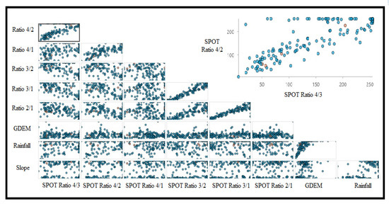
Figure 8.
Results of the collinearity analysis for some explanatory variables.
4.2. Variable Importance of Explanatory Variables
The RF Variable importance for variable Yi is calculated following the equation of [34]:
where VImp (Yj) is variable importance for variable Yj, “ntree” is the number of trees,” errOOBt” is an error when all the factors are included, and “errOOBtj” denotes an error after removal of the variable j. Figure 9 shows the variable importance percentage of the explanatory variables during the prediction stage at ntree = 1000. SPOT-band3, Rainfall, SPOT-band4, SPOT 3/2, PC4, and PC2 images are the most important variables contributing values reaching 11%, 8%, and 7% respectively.
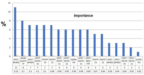
Figure 9.
Variable importance results.
4.3. Random Forest Model Implementation and Generation of GWPM
The Random Forest model is implemented using a reference variable containing about (168 points) of groundwater potential and non-potential locations. The model was trained using 70% of these points and is validated using the rest (30%). Eighteen explanatory variables are tested for groundwater potential mapping. Table 2 lists the range of values covered by each explanatory variable used to train and validate the model. The percentage of overlap between the values used for training and the values used for validation are shown in the shared column. In the GDEM elevation variable, 74% of values that are used to train the model were used to validate the model. A value of prediction that is greater than one indicated that the model predicted values outside the range of values in the training data.
Table 2.
Explanatory Variable Range Diagnostics.
Table 3 shows the RF model characteristics (number of trees, leaf size, tree depth range, mean tree depth, number of randomly sampled variables, and the % of training data excluded for validation in addition to the out-of-bag errors). The default value of Minimum Leaf Size is (1). The maximum tree depth under the default number of trees ranges between 1 and 7. The default percentage of training available per tree is 100%. The number of randomly sampled variables is 4 and it specifies the number of explanatory variables used to create each decision tree. In the present study, 30% of training data was excluded for validation of the model. The default value for the number of trees is 100. The model runs more than one time with a different number of trees to reach the stability of the model. Figure 10 shows the root mean square error (MSE) values at different runs. It scores values 4.944, 4.932, 3.798, and 4.022 at 50, 100, 500 & 1000 trees, respectively. Generally, an increasing number of trees in the Random Forest model provide a more accurate model prediction.
Table 3.
Random Forest model characteristics.
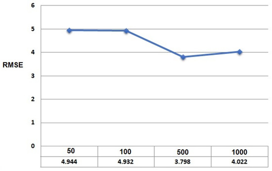
Figure 10.
Root mean square error (MSE) with different trees.
Figure 11 shows the result of the groundwater potential map for the study area generated using the Random Forest model. It shows three main groundwater potential zones: high, moderate, and low/non-potential.
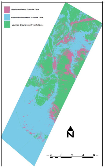
Figure 11.
Groundwater potential zones derived using RF model.
5. Discussion
Groundwater potential mapping is an important for groundwater management. Groundwater storage are affected by many geo-environmental factors namely expanatory variables. Most of these variables are prepared from satellite data in the form of continous or categorical data. Nearly all previous GWPM studies used these explanatory variables in the form of continous or categorical data. These studies performed a pre-processing scaling step before running the ML models [35,36,37,38]. The present study presented approach that utilized explanatory variables as a continous data prepared from original satellite data using remote sensing techniques (band ratios-PCA & NDVI). Simply, it utilized the primary data (raster satellite) instead of secondary data to avoid errors that arose during preparation of categorical data. Each type of satelite data is utilized to prepare some variables that influenced the GWPM. E.g., SPOT satellite data is utilized to generate images that represent lithological and structural variables via band ratios and PCA remote sensing techniques. This study depends on datasets generated from SPOT 5 satellite data, ASTER GDEM, and TRMM rainfall data. Eighteen explanatory variables were tested for groundwater potential mapping. The model was trained using 70% and validated using 30%. The RF model was run several times using different numbers of trees (50, 100, 500, and 1000).
Figure 11 shows the groundwater potential zones derived using RF model. A high groundwater potential zone (red) occurs around Abu Helal and Shaikh Said farms. It extends from the northern part of the study area to the dykes area. The high groundwater potential zone covers an area of about 46.35 km2 representing about 11.5%, of the total study area. This zone is a nearly flat area and has a low slope allowing the water from rainfall and runoff to infiltrate into the soil to reach the shallow water table aquifer. The low/non-groundwater potential zone is represented by the dyke region in the middle part of the study area and the basement rocks distributed to the east and west of Wadi Yalamlam. It occupies an area of about 115 km2, representing about 28.6% of the study area. The fracture system in this zone is represented by faults and joints that permit the water to infiltrate into the deep aquifer. A moderate groundwater potential zone occurs to the south of dyke region to Jeddah-Al-Laith highway, and it occupies an area of about 242.2 km2 representing about 59.9% of the study area. The moderate zone is a flat coastal area with a low slope allowing the water from runoff and rainfall to infiltrate into the shallow water table aquifer. Due to the presence of dykes cutting the wadi path, the amount of water that reaches this zone is limited compared to the high potential zone. The majority of the high and moderate zones lie within the pumping rate range between 10 and 20 m3/day. Figure 12 shows the confusion matrix generated to evaluate the performance of the RF model based on the validation data 30%. The accuracy, sensitivity, and F1_score (Table 4) are all generated and evaluated and proved that the model is the best fit with an overall accuracy of 96.1%.
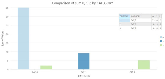
Figure 12.
Confusion matrix showing groundwater potential classes.
Table 4.
Results of validation methods used to evaluate the performance of the RF model.
6. Conclusions
The present study proved the usefulness of the RF model and the satellite data in identifying groundwater potential zones in arid/hyper-arid regions. The approach developed in the present study successfully identifies the geological, topographical, and climatic factors that influenced groundwater storage. The authors encourage the researchers to apply this approach under different climatic conditions. The main conclusions of this study are (1) The RF model successfully classified the study area into three groundwater potential zones (high, moderate & low) with an accuracy of 96%. (2) The majority of high and moderate classes lie within the pumping rate range between 10 and 20 m3/day. (3) This study can be applied to any other wadis having the same conditions to help the decision-makers in planning the development projects.
Author Contributions
Conceptualization, A.M.; methodology, A.M.; software, A.M.; validation, A.M.; investigation, A.M. and B.N.; resources, A.M. and B.N.; data curation, A.M. and B.N.; writing—original draft preparation, A.M.; writing—review and editing, A.M. and B.N.; visualization, A.M.; supervision, A.M. All authors have read and agreed to the published version of the manuscript.
Funding
This research received no external funding.
Institutional Review Board Statement
Not applicable.
Informed Consent Statement
Not applicable.
Data Availability Statement
Not applicable.
Conflicts of Interest
The authors declare no conflict of interest.
References
- Bayumi, T. Quantitative Groundwater Resources Evaluation in the Lower Part of Yalamlam Basin, Makkah Al Mukarramah, Western Saudi Arabia. JKAU Earth Sci. 2008, 19, 35–56. [Google Scholar] [CrossRef]
- Subyani, A.M.; Bayumi, T. Physiographical and Hydrological Analysis of Yalamlam Basin, Makkah Al-Mukarramah area. JKAU Earth Sci. 2001, 13, 151–177. [Google Scholar] [CrossRef]
- Yani, A.M.; Bayumi, T. Evaluation of Groundwater Resources in Wadi Yalamlam Basin, Makkah Area; Unpublished Project No. (203/420); King Abdulaziz University: Jeddah, Saudi Arabia, 2001. [Google Scholar]
- Subyani, A. Study Evaluation of Groundwater Resources in Wadi Yalamlam and Wadi Adam Basins, Makkah Al-Mukarramah, Al-Mukarramah Area. In Proceedings of the International Conference on Water Resources & Arid Environment Riyadh, Riyadh, Saudi Arabia, 5–8 December 2004. [Google Scholar]
- Madani, A.; Niyazi, B. Groundwater potential mapping using remote sensing 897 techniques and weights of evidence GIS model: A case study from Wadi Yalamlam 898 basin, Makkah Province, Western Saudi Arabia. Environ. Earth Sci. 2015, 74, 5129–5142. [Google Scholar] [CrossRef]
- Madani, A.A.; Niyazi, B.; Elfakharani, A.; Osman, H. The effects of structural elements on groundwater of Wadi Yalamlam, Saudi Arabia using integration of remote sensing and airbornemagnetic survey. Earth Syst. Environ. J. 2019, 3, 301–312. [Google Scholar] [CrossRef]
- Rajmohan, N.; Masoud, M.; Niyazi, N. Appraisal of groundwater quality and health risk in the Yalamlam basin, Saudi Arabia. Environ. Sci. Pollut. Res. 2022, 29, 83653–83670. [Google Scholar] [CrossRef]
- Arulbalaji, P.; Padmalal, D.; Sreelash, K. GIS and AHP Techniques Based Delineation of Groundwater Potential Zones: A case study from Southern Western Ghats, India. Sci. Rep. 2019, 9, 2082. [Google Scholar] [CrossRef]
- Mallick, J.; Khan, R.A.; Ahmed, M.; Alqadhi, S.D.; Alsubih, M.; Falqi, I.; Hasan, M.A. Modeling Groundwater Potential Zone in a Semi-Arid Region of Aseer Using Fuzzy-AHP and Geoinformation Techniques. Water 2019, 11, 2656. [Google Scholar] [CrossRef]
- Benjmel, K.; Amraoui, F.; Boutaleb, S.; Ouchchen, M.; Tahiri, A.; Touab, A. Mapping of Groundwater Potential Zones in Crystalline Terrain Using Remote Sensing, GIS Techniques, and Multicriteria Data Analysis (Case of the Ighrem Region, Western Anti-Atlas, Morocco). Water 2020, 12, 471. [Google Scholar] [CrossRef]
- Melese, T.; Belay, T. Groundwater Potential Zone Mapping Using Analytical Hierarchy Process and GIS in Muga Watershed, Abay Basin, Ethiopia. Glob. Chall. 2022, 6, 2100068. [Google Scholar] [CrossRef]
- Morgan, H.; Hussien, H.M.; Madani, A.; Nassar, T. Delineating Groundwater Potential Zones in Hyper-Arid Regions Using the Applications of Remote Sensing and GIS Modeling in the Eastern Desert, Egypt. Sustainability 2022, 14, 16942. [Google Scholar] [CrossRef]
- Naghibi, S.A.; Pourghasemi, H.R. A comparative assessment between three machine learning models and their performance comparison by bivariate and multivariate statistical methods in groundwater potential mapping. Water Resour. Manag. 2015, 29, 5217–5236. [Google Scholar] [CrossRef]
- Naghibi, S.A.; Moghaddam, D.D.; Kalantar, B.; Pradhan, B.; Kisi, O. A comparative assessment of GIS-based data mining models and a novel ensemble model in groundwater well potential mapping. J. Hydrol. 2017, 548, 471–483. [Google Scholar] [CrossRef]
- Lee, S.; Hong, S.M.; Jung., H.S. GIS-based groundwater potential mapping using artificial neural network and support vector machine models: The case of Boryeong city in Korea. Geocarto Int. 2018, 33, 847–861. [Google Scholar] [CrossRef]
- Nguyen, P.T.; Ha, D.H.; Jaafari, A.; Nguyen, H.D.; Van Phong, T.; Al-Ansari, N.; Prakash, I.; Le, H.V.; Pham, B.T. Groundwater potential mapping combining artificial neural network and real AdaBoost ensemble technique: The DakNong Province case-study, Vietnam. Int. J. Environ. Res. Public Health 2020, 17, 2473. [Google Scholar] [CrossRef]
- Arabameri, A.; Lee, S.; Tiefenbacher, J.P.; Ngo, P.T.T. Novel ensemble of MCDM-Artificial Intelligence techniques for groundwater potential mapping in arid and semi-arid regions (Iran). Remote Sens. 2020, 12, 490. [Google Scholar] [CrossRef]
- Martínez-Santos, P.; Renard, P. Mapping Groundwater Potential Through an Ensemble of Big Data Methods. Groundwater 2020, 58, 583–597. [Google Scholar] [CrossRef] [PubMed]
- Moghaddam, D.D.; Rahmati, O.; Panahi, M.; Tiefenbacher, J.; Darabi, H.; Haghizadeh, A.; Haghighi, A.T.; Nalivan, O.A.; Bui, D.T. The effect of sample size on different machine learning models for groundwater potential mapping in mountain bedrock aquifers. Catena 2020, 187, 104421. [Google Scholar] [CrossRef]
- Singh, R. Assessing the impact of drought conditions on groundwater potential in Godavari Middle Sub-Basin, India using analytical hierarchy process and random forest machine learning algorithm. Groundw. Sustain. Dev. 2021, 13, 100554. [Google Scholar]
- Morgan, H.; Madani, A.; Hussien, M.; Nassar, T. Delineating Groundwater Potential zones using an ensemble machine learning model for groundwater management sustainability of East Idfu–Esna Region, Nile Valley, Upper Egypt. Geosci. Lett. 2022, 14, 16942. [Google Scholar]
- Bai, Z.; Liu, Q.; Liu, Y. Groundwater potential mapping in Hubei region of China using machine learning, ensemble learning, deep learning and AutoML methods. Nat. Resour. Res. 2022, 31, 2549–2569. [Google Scholar] [CrossRef]
- Kumar, C.P. Estimation of natural ground water recharge. ISH J. Hydraul. Eng. 1997, 3, 61–74. [Google Scholar] [CrossRef]
- Jyrkama, M.I.; Sykes, J.F.; Normani, S.D. Recharge estimation for transient ground water modeling. Groundwater 2002, 40, 638. [Google Scholar] [CrossRef] [PubMed]
- Madani, A.A. Geological Studies and Remote Sensing Applications on Wadi Natash Volcanic, Eastern Desert, Egypt. Ph.D. Thesis, Faculty of Science, Cairo University, Cairo, Egypt, 2001. [Google Scholar]
- Madani, A.A. Knowledge-driven GIS modeling technique for gold exploration, Bulghah gold mine area, Saudi Arabia. Egypt J. Remote Sens. Space Sci. 2011, 14, 91–97. [Google Scholar] [CrossRef]
- El Sobky, M.A.; Madani, A.A.; Surour, A.A. Spectral characterization of the Batuga granite pluton, South Eastern Desert, Egypt: Influence of lithological and mineralogical variation on ASD Terraspec data. Arab. J. Geosci. 2020, 13, 1246. [Google Scholar] [CrossRef]
- Drury, S. Image Interpretation in Geology, 2nd ed.; Chapman and Hall: London, UK, 1993. [Google Scholar]
- Breiman, L. Random Forests. Mach. Learn. 2001, 45, 5–32. [Google Scholar] [CrossRef]
- Carranza, E.J.; Laborte, A.G. Random forest predictive modeling of mineral prospectivity with small number of prospects and data with missing values in Abra (Philippines). Comput. Geosci. 2015, 74, 60–70. [Google Scholar] [CrossRef]
- Prasad, P.; Loveson, V.J.; Kotha, M.; Yadav, R. Application of machine learning techniques in groundwater potential mapping along the west coast of India. GISci. Remote Sens. 2020, 57, 735–752. [Google Scholar] [CrossRef]
- Martínez-Santos, P.; Díaz-Alcaide, S.; De la Hera, A.; Gomez-Escalonilla, V. A multi-parametric supervised classification algorithm to map groundwater-dependent wetlands. J. Hydrol. 2021, 603, 126873. [Google Scholar] [CrossRef]
- Dormann, C.F.; Elith, J.; Bacher, S.; Buchmann, C.; Carl, G.; Carré, G.; Marquéz, J.R.G.; Gruber, B.; Lafourcade, B.; Leitão, P.J.; et al. Collinearity: A review of methods to deal with it and a simulation study evaluating their performance. Ecography 2013, 36, 27–46. [Google Scholar] [CrossRef]
- Van Beijma, S.; Comber, A.; Lamb, A. Random forest classification of salt marsh vegetation habitats using quad-polarimetric airborne SAR, elevation and optical RS data. Remote Sens. Environ. 2014, 149, 118–129. [Google Scholar] [CrossRef]
- Angelis, L.; Stamelos, I. A simulation tool for efficient analogy based cost estimation. Empir. Softw. Eng. 2000, 5, 35–68. [Google Scholar] [CrossRef]
- Pedregosa, F.; Varoquaux, G.; Gramfort, A.; Michel, V.; Thirion, B.; Grisel, O.; Blondel, M.; Prettenhofer, P.; Weiss, R.; Dubourg, V.; et al. Scikit-learn: Machine Learning in Python. J. Mach. Learn. Res. 2011, 1045, 2825–2830. [Google Scholar]
- Huang, J.; Li, Y.F.; Xie, M. An empirical analysis of data preprocessing for machine learning-based software cost estimation. Inf. Softw. Technol. 2015, 67, 108–127. [Google Scholar] [CrossRef]
- Zheng, A.; Casari, A. Feature Engineering for Machine Learning; O’Reilly Media, Inc.: Sebastopol, CA, USA, 2018; p. 218. [Google Scholar]
Disclaimer/Publisher’s Note: The statements, opinions and data contained in all publications are solely those of the individual author(s) and contributor(s) and not of MDPI and/or the editor(s). MDPI and/or the editor(s) disclaim responsibility for any injury to people or property resulting from any ideas, methods, instructions or products referred to in the content. |
© 2023 by the authors. Licensee MDPI, Basel, Switzerland. This article is an open access article distributed under the terms and conditions of the Creative Commons Attribution (CC BY) license (https://creativecommons.org/licenses/by/4.0/).