Article

Downscaling of Hourly Climate Data for the Assessment of Building Energy Performance

ENEA C.R. Casaccia, Via Anguillarese 301, 00123 Rome, Italy
*
Author to whom correspondence should be addressed.
Sustainability 2023, 15(3), 2762; https://doi.org/10.3390/su15032762
Submission received: 23 December 2022 / Revised: 18 January 2023 / Accepted: 31 January 2023 / Published: 3 February 2023
(This article belongs to the Special Issue Built Environment and Sustainability)

Abstract

:
In Italy, the calculation of the energy needs of buildings has been mainly based on quasi-steady state calculation procedures. Nowadays, the increasing interest in more detailed energy analysis for high-efficiency buildings requires more accurate calculation methods. In this work, starting from the hourly data of UNI 10349, the downscaling of a typical meteorological year was carried out by applying different mathematical and physical models for the main climate variables considered in the energy balance of a building to be used in dynamic simulation tools. All results were validated with one-minute measurements observed at the ENEA Research Centre in Rome, Italy. The results showed an MBE% of 0.008% and RMSE% of 0.114% using the interpolation spline method for the temperature, while, for the global horizontal irradiance, applying the novel sinusoidal–physical interpolation method showed an MBE% of −0.4% and an RMSE% of 31.8% for the 1 min observation data. In this paper, an easily implemented novel model for downscaling solar irradiance for all sky conditions that takes into account the physical aspects of atmospheric phenomena is presented.

1. Introduction

This study aimed at downscaling climatic quantities to be used in the energy analysis of high-efficiency buildings. The national technical standards [1,2,3,4] provide monthly climate data and cumulative indicators (heating degree day, climate severity index, etc.) for the main quantities that affect the energy balance of buildings, but up to now, no climatic quantities are available on a sub-hourly scale. The application of advanced calculation methods for the building’s energy needs, such as dynamic methods, requires more accurate input data for thermo-energy simulations [5,6]. To this end, the availability of climate data on a short time scale would allow for the best use of the finest calculation systems, which are becoming increasingly popular. This aspect is also particularly relevant if the considered power plants are based on the use of renewable sources, such as heat pumps, photovoltaic modules, and geothermal systems, whose performances are strictly linked to weather conditions and climatic variations in the site where the building is located [7,8,9].
Historical solar resource data are scarce and if they are available, they are only at an hourly time scale. This is the case for data included in a typical meteorological year (TMY) [10,11] and in many widely used models derived from satellite information. One-minute historical data of TMY variables are almost impossible to find. High-temporal-resolution solar data in TMY data are required for both the planning and operation of large-scale systems in building energy savings, concentrated solar thermal plants (CSP) and solar photovoltaic systems (PV). However, hourly solar irradiance data does not capture the transient effects of clouds well enough to properly design and manage large-scale systems (CSP, PV, buildings). Hourly time resolution could be unsatisfactory in simulating transient processes in a power plant. Some solar systems are particularly sensitive to cloud transience, and thus, power plant performance requires input with higher temporal resolution than what is now available with a one-hour time resolution.
We identified different downscaling models that consider different climatic variables to derive sub-hourly climatic quantities. Our method started from hourly and minute-scale data pairs in ENEA, Casaccia (Rome, Italy), where observed meteorological variables are available. Hourly values correspond to each 60 min of data. In particular, mathematical spline interpolation methodologies were used for temperature and humidity, while innovative and unique models were applied for all three components of solar radiation for all sky conditions. In this study, we considered only temperature and global irradiance. The generated syntactical minute quantities were validated with the minute measurements. Subsequently, using the presented methodologies, it is possible to obtain the TMY (starting from the corresponding hourly scale values of UNI 10349) with modeled sub-hourly values that nowadays become highly important in the energy analysis of high-efficiency buildings. No study could be found that generated high-temporal-resolution pairs of irradiance data for locations where only hourly data existed. Several studies were proposed to address the need for solar data with a higher temporal resolution [12]. In the literature, many mathematical algorithms were used to generate synthetic solar irradiance [13,14,15], different stochastic downscaling methods [16] or complex mathematical models for application [17]. However, the majority of these algorithms available in the literature generate synthetic hourly data starting from measured daily radiation [13,14,15] or even from the daily average fraction between the ratio of solar radiation that reaches the surface of Earth and the extraterrestrial radiation that reaches the top of the atmosphere (clearness index) [14].
This work introduced new applications and approaches for calculation methodologies and the possibility to satisfy new standard needs in climate zones in the national Italian territory, proposing a new standard for new technologies and building constructions [1,2,3,4,18]. See the end of the document for further details about references.

2. Materials and Methodology

The study for the downscaling of the hourly climate data was divided into 4 phases:
  • Preliminary analysis of the minute measurements;
  • Selection of downscaling models;
  • Validation with measurements (city of Rome);
  • Data processing to obtain sub-hourly climate variables (scales: 15 min, 20 min and 30 min).
In the first phase of the work, the minute measurements (2017–2019) carried out in C.R. ENEA, Casaccia (Rome), were analyzed to check for any outlier values and highlight the main descriptive statistics of the data [19].
Furthermore, a whole annual data set was selected to verify the variability of the different climatic quantities. As expected, the air temperature and the specific humidity showed very low variability at the hourly time scale (Figure 1), while the solar radiation was found to be much more variable, as it depended on the sky conditions of the day considered.
Based on these findings, different downscaling models were developed to process the sub-hourly scale temperature, specific humidity and solar radiation.
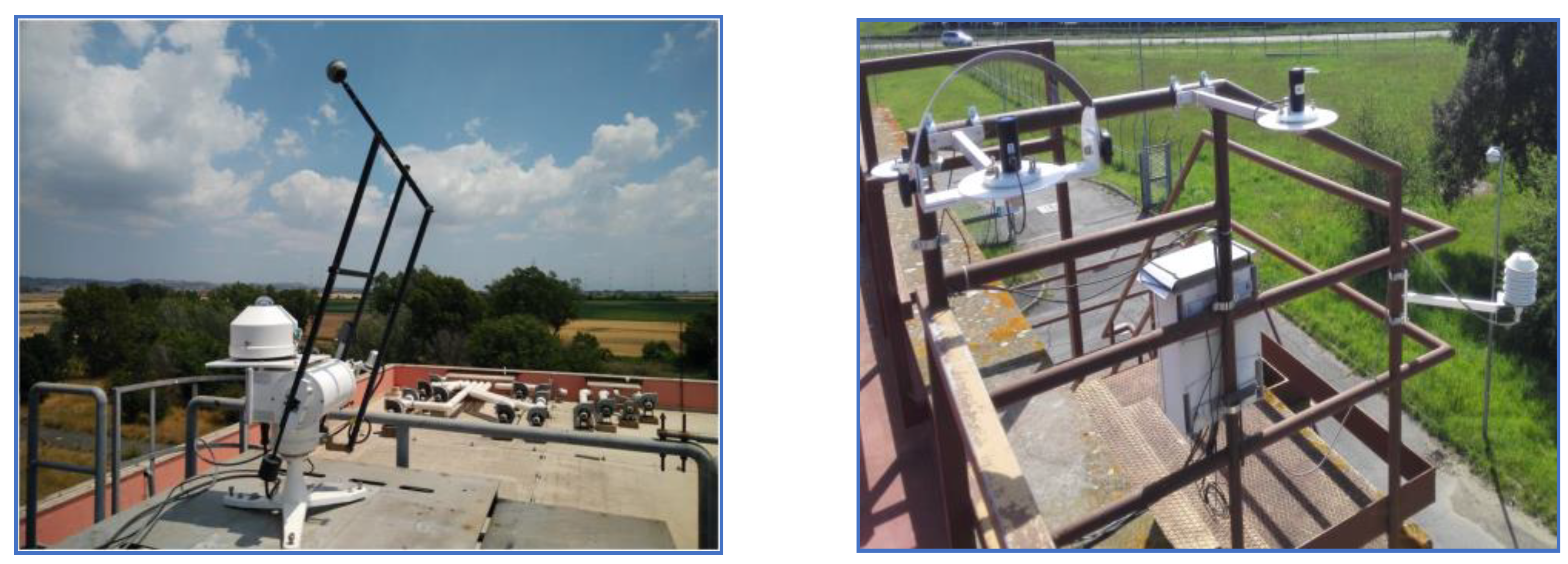
In the ENEA research center, the monitoring of meteorological variables (temperature (T), humidity (U), wind speed (Ws) and direction (Wd), etc.) and solar radiation (global solar irradiation on a horizontal plane (GHI), direct irradiation on a normal surface (DNI) and diffuse irradiation on a horizontal plane (DfHI)) have been available since 2008 [20]. Figure 2 shows the installed solar-metric observation instruments. The installed weather station consists of EKO instruments. A solar-metric instruments count one pyrheliometer (DNI) set on a Sun tracker and two pyranometers (GHI and shaded for DfHI). The sun tracker has a double aim, which allows the instrumentation to be aimed in the direction of the Sun, while the shaded ball pointing to one of the two pyranometers allows for measuring diffuse horizontal irradiance. The EKO instruments measure the solar irradiance in a spectral range from 335 to 2200 nm within an error of ±3% [21]. The solar-metric instrument is calibrated on regular basis every several years. All observed variables are stored in a vast database with different time scales.
The measures relating to different years at the minute time scale were preliminarily evaluated to verify the consistency of the data and the presence of any outliers and the year 2018 was chosen. Subsequently, the analysis was focused on the typical profiles of the different climatic quantities that were most influential in the energy balance of buildings. Temperature and solar radiation are the primary sources of energy for solar systems and are the main climate variables for calculating the energy needs of buildings [22,23]; for these reasons, it is important to measure and estimate these resources with high accuracy.
The considered variables in this study, namely, T, U and GHI, are completely different in their natures and different approaches are needed for their processing. For example, the temperature has a daily and annual “sinusoidal” shape, while global horizontal irradiance values are presented as a bell curve. The GHI strongly depends on atmospheric conditions, such as cloud cover, humidity, presented pollution and aerosols in the atmosphere. The differences in the natures of the variables are expressed using the statistical measures in Table 1, where, for example, the daily ranges for T were −5 °C up to 36 °C, while for GHI, the range was from 0 W/m2 up to 1210 W/m2.
In the considered 2018 database related to temperature, two very short periods of missing data were found that did not harm the representativeness of the hourly data that were used here as input; in fact, missing data were 0.23% of the total number of 1 min observations for that year (525,600 data points).

3. Results and Discussion

3.1. Temperature and Humidity Downscaling

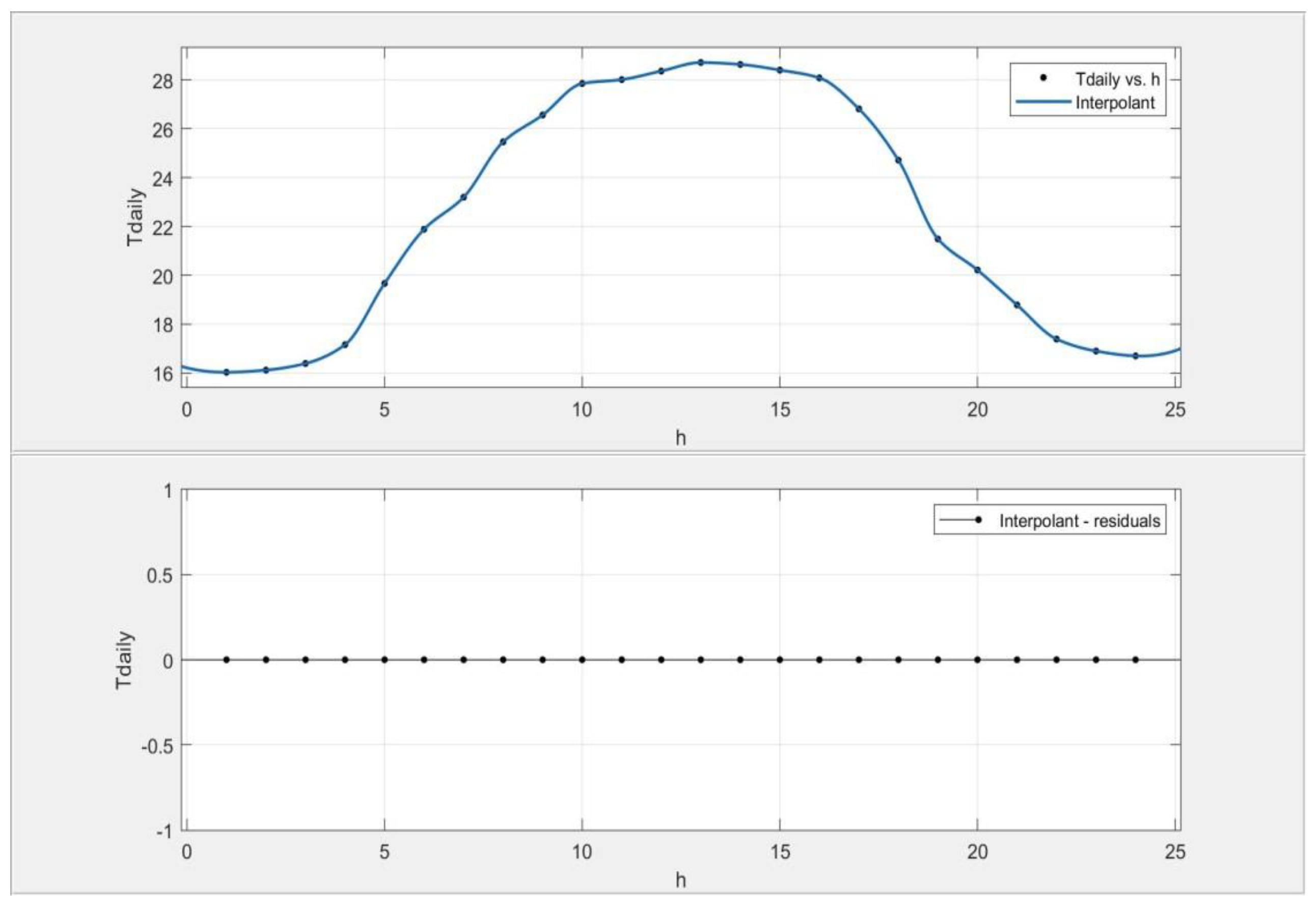
The general problem that we intended to solve was to determine an analytical expression of the function y = f(t) in order to describe the time course of the observed climatic variable of which we know a finite number of points, namely, their observed hourly values (Figure 3). The downscaling of sub-hourly data, starting from those on an hourly scale, can be carried out by applying different fitting models. The choice of the most appropriate model clearly depends on the data characteristics to be processed, but also on the application and the purposes of output data. A class of functions that are widely used to best interpolate the discrete trend of the measured quantity are spline functions, which essentially consist of a set of piecewise polynomials with specific regularity. The application of this well-known approach provides the subdivision into sub-intervals of the defined field for the quantity to be interpolated y = f(t) through nodes called spline nodes. In our case, we considered the measured points (hourly values) as nodes of spline interpolation, while the intervals were those between two consecutive points (consecutive hourly values), which we wanted to interpolate with algebraic curves of polynomial type with degree n ≤ 3:
f ( x ) = a + b x + c x   2 + d x   3
In the preliminary phase, different mathematical interpolation models were used by applying them to different time scales.
Despite the fact that the use of linear splines seems to be adequate to interpolate daily data, the need to directly process a more articulated set of data, as happens, for example, when analyzing data on a monthly, seasonal or annual scale, suggests using cubic spline functions that allow for optimizing the interpolation and obtaining an excellent reconstruction of sub-hourly trend.
This reason led to the choice of the piecewise cubic Hermite interpolating polynomial (PSHIP) interpolation spline function [24] implemented in the MATLAB environment for processing the typical climate years TMY of the different Italian locations.
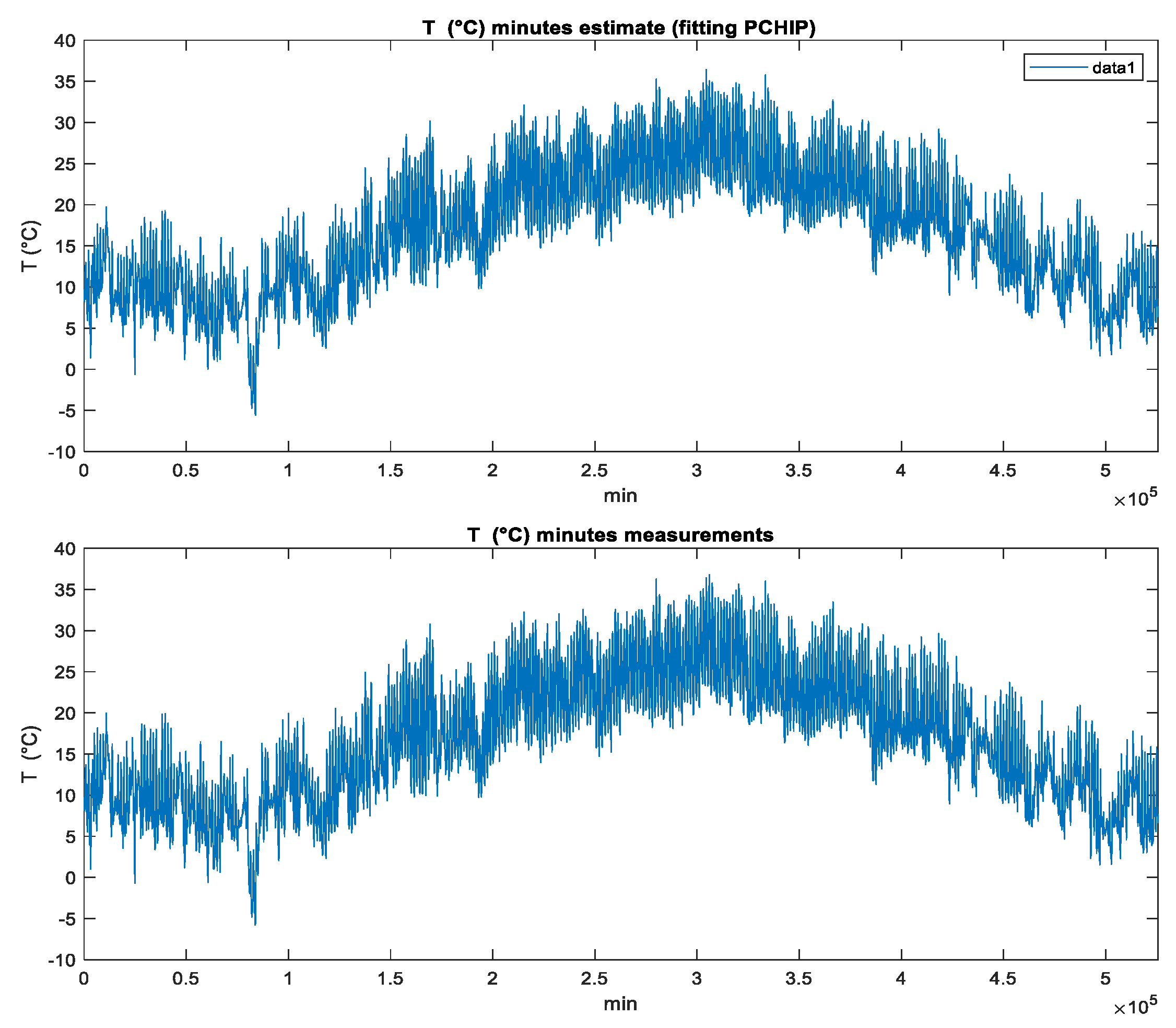
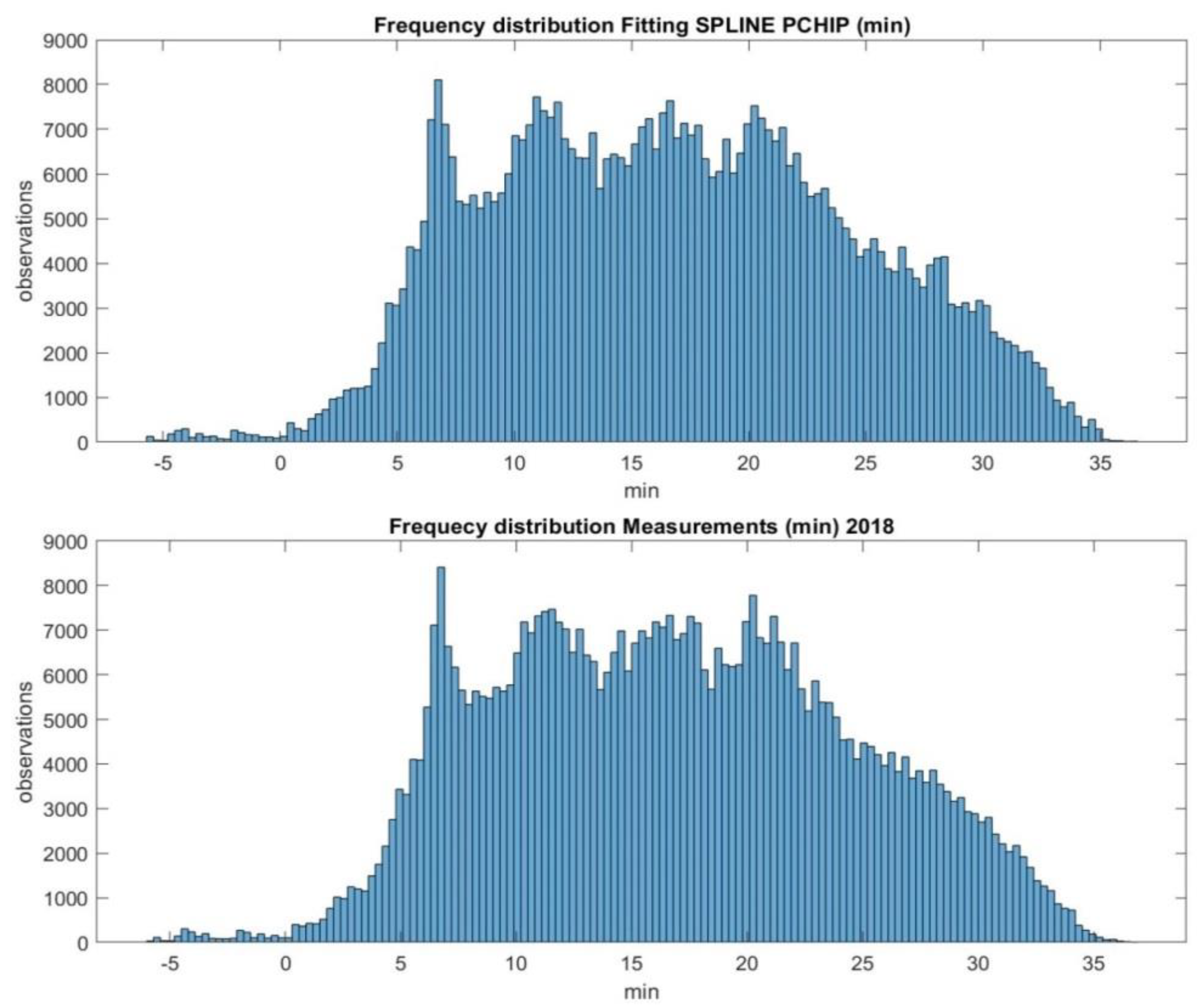
The two graphs shown below (Figure 4 and Figure 5) show the results obtained using PSHIP interpolation with an annual interval, both in terms of the time trend per minute and in terms of relative frequencies, starting from hourly data. The interpolation of the entire data interval of hourly to minute-scale measurements showed excellent “overlap” of the signal obtained using the presented interpolation for temperature.

3.2. Solar Radiation Sub-Hourly Interpolation Methods

The mathematical interpolation methods that were described in the previous section were shown to be adequate for temperature but this was not valid for solar radiation. The trend of solar radiation depends essentially on the atmospheric conditions, in particular, on the sky specification and its cloud phenomena. The nature of cloud phenomena is unpredictable in occurrence and intensity over time and its trend is largely irregular [25,26]. Therefore, the trend of irradiance is hardly “catchable” with a purely mathematical model [27]. Consequently, purely mathematical interpolation cannot be the right choice for solar radiation.
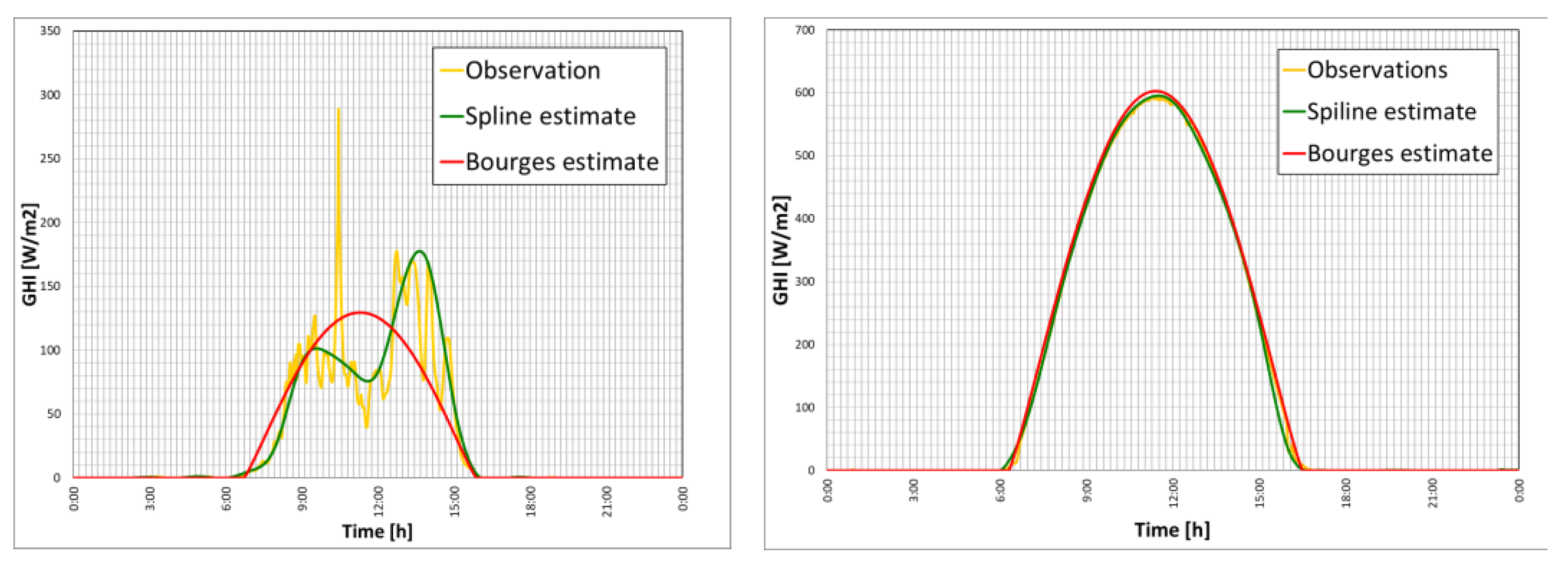
The literature presents different physical models that consider solar radiation. One of them is the Bourges model, which is one of the widely and well-known physical models for irradiance [28]. Up to now, there is no published work where this model is used to downscale irradiance to a sub-hourly frequency. In Figure 6, we present the performance of the Bourges physical model together with the cubic interpolation against the 1 min frequency measurements for the examples of a partially cloudy day (on the left) and a day with clear sky conditions (on the right). The synthetic trends obtained using a cubic spline and physical Bourges model interpolations starting from hourly data were superimposed for the day with clear sky conditions with minute measurements, but the outcome was not as satisfactory for a day with cloudy sky conditions. Figure 6 shows that assessing synthetic sequences on solar data is not as straightforward as assessing other meteorological variables, such as atmospheric temperature, where variation in atmospheric conditions is less pronounced. Synthetic solar data with the mathematical and physical models do not correspond for all cloud conditions for one-minute time intervals. This similar behavior is also present for two other solar components (direct and diffuse irradiance) not shown here.
Several studies were proposed to address the need for solar data with a higher temporal resolution and to summarize many algorithms that were used to generate synthetic irradiance, as well as develop their own. Some of those studies used different stochastic methods (Markov chain or autoregressive models), time-dependent autoregressive Gaussian method and Fourier analysis to construct a synthetic time series of irradiance data. However, the majority of these algorithms, and other similar algorithms in the literature [13,14,15,29], generate synthetic hourly data from measured daily radiation or the daily average clearness index. All methods available in the literature try to fill the gaps between the generally available data resources and the parameters requested using solar applications. Up to now, no study could be found that generated high temporal resolution pairs of irradiance data for locations where only hourly data existed. In the literature, some studies used the sky condition “stages” to apply the different mathematical approaches, where sky stages are categorized using the normalized clearness index [14] and clear sky index [15].
Table 2 presents the identification of different sky conditions with a daily clearness index (kc) for 2018. The clearness index has a range of 0 to 1, where 1 denotes a clear sky and 0 denotes completely covered conditions. By considering the identification of the sky, we observed 120 days with clear sky conditions and 242 days with cloudy sky conditions in 2018 at the location in Casaccia.
Within the presented data, where a high number of cloudy days was present (Table 2), purely mathematical and widely used physical models for solar data could not provide a satisfactory interpolation of the data for the entire year. Although under clear sky conditions, the synthetic interpolation of 1 min irradiance values was generated well using a simple cubic or even linear interpolation from hourly values, the method to select clear sky conditions with kc was valid only when the clear sky remained for the entire Sun duration. In order to be able to downscale irradiance for all sky conditions, we moved one step forward. In fact, for any cloud condition, the physical model for a global horizontal irradiance at the ground (I) is
I = K T I o
where I0 is the corresponding extra-atmospheric irradiance and KT is the global transmission coefficient, which, for whatever conditions, can be written as a product of KTc for the condition of clear sky and a factor kc that takes into account the contingent presence of clouds:
K T = K T c k c = B k c cos 0.15 ϑ z
where B is the parameter introduced by Bourges, used above, and which coincides with KTc in the hypothetical conditions of the Sun at the zenith, i.e., when the zenith angle θz is zero. The hourly values of B are easily calculated from the hourly GHI data or obtained from tables already available for all locations thanks to the series of multi-year measurements. Rewriting and collecting the above expressions, we could write
I = I o n S cos 1.15 ϑ z
in which the product Bkc was collected in the symbol S, and considering that the horizontal and normal extra-atmospheric irradiances (Ion) are linked with the formula I0 = Ion cosθz. Finally, we introduce the interpolation method that will propose a “plausible” interpolation (Sh) starting from hourly values of global horizontal irradiations Ih as
S h = I h I o n cos 1.15 ϑ z , h
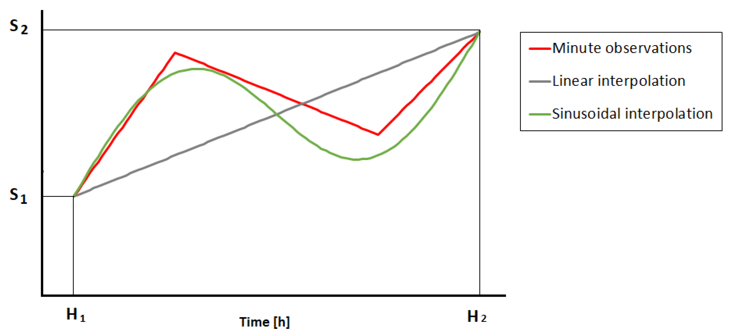
Obviously, as we have already seen, the possible linear interpolation that joins the consecutive pairs of hourly values (Sh, Sh+1) fits well only for clear skies but it is absolutely inadequate to “capture” the irregular trends of ups and downs when cloudy sky conditions are present between consecutive hours. An interpolating trend was therefore proposed that overlapped the linear interpolation in the first approximation with a sine curve period. The graphical methodology of this novel interpolation is presented in Figure 7, where the minute measurements are presented with a red line, linear interpolation is presented in gray and the proposed “sinusoidal” interpolation is presented in green. This methodology could be applied to any variable that has irregularity in its nature and at any time scale. The proposed methodology is able to catch the unpredictable irregularity in the trend of solar data while traditional mathematical models cannot.
S i = S 1 + S 2 S 1 H 2 H 1 i H 1 + A s e n 2 π H 2 H 1 i H 1
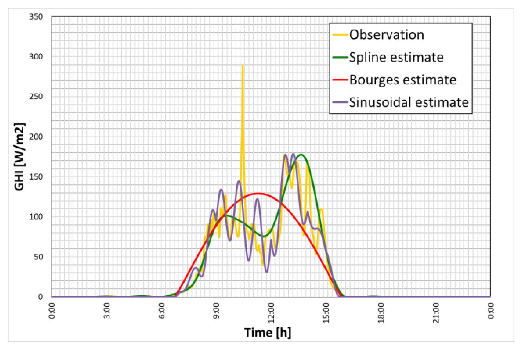
The formulation of the proposed methodology is mathematically presented in Equation (6). H1 and H2 are two consecutive hourly instants to which the known values correspond to two consecutive hours where S1 and S2 were derived from Equation (5). i is any instant between the hourly extremes H1iH2. The parameter A determines the amplification of the sinusoidal correction to the linear trend. The absolute value of A is calculated as the ratio between the difference in the measured hourly global horizontal irradiance (our input data) and the hourly values calculated with the parameter (Sh) that varies linearly between (Sh, Sh+1) and the daily average of the measured hourly global horizontal irradiance. For example, when the condition is kc > 0.7 (clear sky) the difference in the numerator is close to zero, and thus, it can be given as A = 0. On the other hand, the parameter A cannot have “large values”, and from an analysis of the results obtained with minute-scale observations, the maximum value of A = 0.08 was obtained. The example of one cloudy day with three different interpolations is presented in Figure 8. We easily observed that the presented sinusoidal model (Figure 8, in purple) “catches” the irregularity in the measured data and fits better than the mathematical spline (in green) and purely physical Bourge model (in red).
In conclusion, when clear sky conditions are presented, even the simple mathematical interpolation (linear or cubic) led to excellent results, while for different sky conditions, this was not sufficient. The models available in the literature often turned out to be artificially complex in conception or not very practical to implement. A new method introduced here called the “sinusoidal–physical model” showed numerous advantages, such as (1) the compactness of the mathematical formulation, which avoids the use of sky-type subdivisions in classes with the consequent need to adopt a different formulation for each; (2) the naturalness with which even the special class of clear skies is incorporated into the method as a special case; and (3) the consequent easy implementation. Table 3 shows the list of interpolation methods examined for solar radiation and the cases when they are applicable.

4. Validation of the Models

The developed interpolating sinusoidal–physical model for the global horizontal irradiance analyzed here was tailored to generate downscaled values for the TMY over the region of Italy at sub-hourly frequencies (here, a 1 min downscaling interval from hourly values is presented).
In order to validate the model, comparisons between measured values and modeled estimated values were carried out. Statistical indices and the dispersion diagram for the air temperature and irradiance are presented here.
The standard statistical indices in terms of the mean bias error (MBE) and root-mean-squared error (RMSE) are demonstrated. The first of these indicators, namely, MBE, is simply the difference between the mean estimate values and the observation values. In our case, the calculated value is
M B E = 1 N i = 1 N E i O i
where N is the total number of observation pairs in the data; the subscript “i” refers to the ith pair; and “O” and “E” refer to the observations and estimated values, respectively. A low value of the MBE means that the measurements and estimates are offset from the average value. Another widely used quality deviation index, namely, RMSE, which considers the squares of the deviations rather than the absolute values in order to attribute a greater weight to higher deviations in the summation, is given as
R M S E = 1 N i = 1 N E i O i 2
We find the percentage error of both statistical indices (MBE% and RMSE%) we when divide our indices with the mean observations and multiply it by 100.
In order to facilitate the readability of the dispersion graph and to easily point out the behavior of modeled estimates, the graphs of temperature and irradiance are presented by adopting criteria that guarantee maximum representativeness of the resulting sample, where data pairs are extracted from the entire annual series.
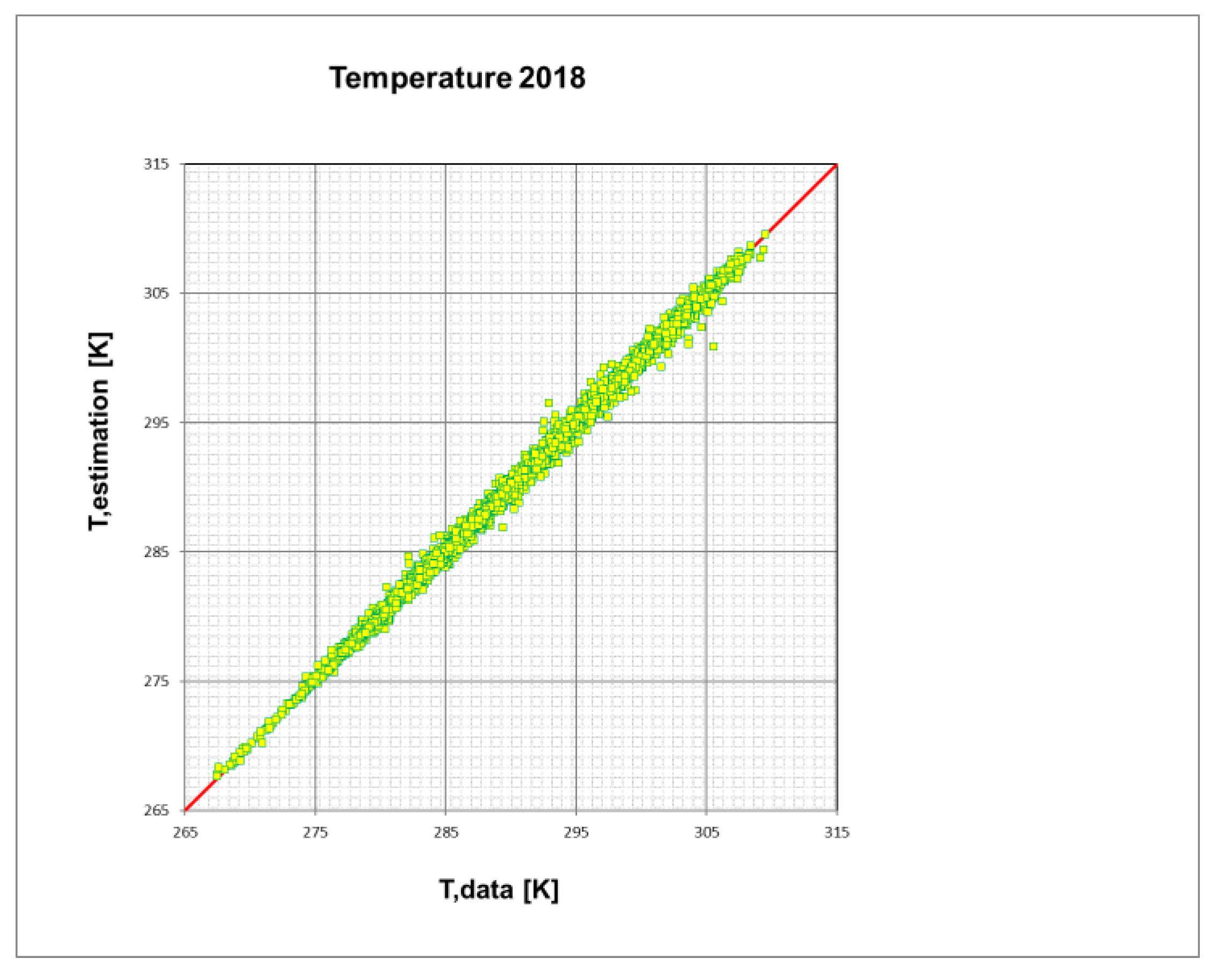
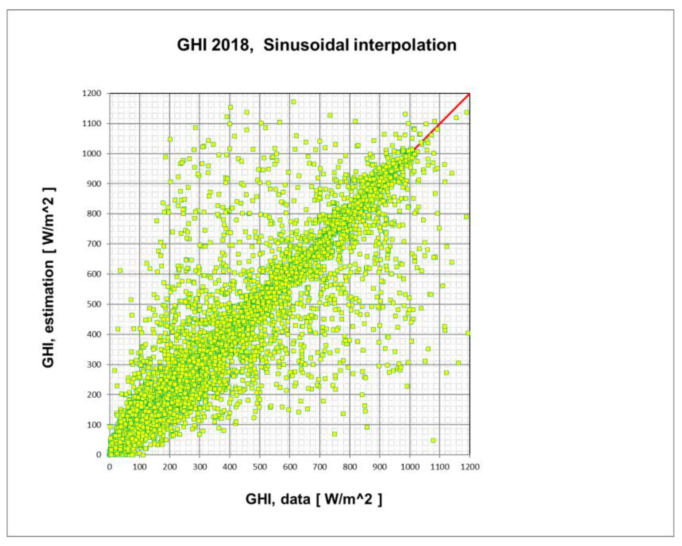
Figure 9 presents the temperature dispersion diagram, where pairs (measure and estimated values) were considered in correspondence with a step of 59 min between one pair and the next one. This step avoided taking points that invariably coincided with the HH:00 instants or determined exact submultiple intervals of the hour. It was easily observed that the estimates and measurements of temperature accurately followed the bisector. With the sample data analysis described, we had 8890 data representatives instead of 521,280 minute-scale data, with an MBE of 0.010 K, RMSE of 0.330 K, MBE% of 0.008% and RMSE% of 0.114% when using PCHIP interpolation for the temperature.
Figure 10 shows the dispersion graph for the global horizontal irradiance for all sky situations. The dispersion irradiance graph presented here was constructed with a more limited number of points than the temperature ones, as night values are always zero. A shorter sampling step of 29 min for the irradiance graph representation was adopted in order to not decrease the number of extracted samples too much. The results argue in favor of the goodness of the interpolation method adopted for the irradiance, although they were not as convincing as those seen for temperature. This result is in line with the nature of the cloudy phenomenon, which in the hourly time step can change rapidly, even several times unpredictably in its intensity. Despite this phenomenon, the MBE and RMSE indices were much lower than the maximum values that the irradiance could assume (up to 1200 W/m2). With the sample data analysis described for the global horizontal irradiance, we had 8653 data representatives instead of 521,280 minute-scale data, with an MBE of −1.4 W/m2, RMSE of 116.9 W/m2, MBE% of −0.4% and RMSE% of 31.8% when using the sinusoidal–physical model. If a subsample was extracted from the sample consisting only of the data of clear days, that is the days with a global transmission coefficient larger than 0.65, the coupling indices improved significantly (not shown here). This improvement was, as repeated several times, due to the easier interpolation when the sky condition was in the absence of clouds.
The presented methods were created in order to easily and accurately downscale the valuable hourly database of TMY given by CTI in support of the UNI 10349 standard to any time scale (10, 15, 20, 30 or even 1 min sub-intervals). As mentioned, the number of TMY datasets with hourly data is 110, one for each Italian province. The procedure for downscaling the data followed different steps:
  • Extraction of the time series of the 8760 hourly data for each quantity;
  • Calculation of the hourly values of mass humidity starting from the relative humidity, pressure and temperature of the air;
  • Calculation of the hourly values of the DNI (normal direct irradiance) starting from the horizontal DI (direct irradiance);
  • Application of the interpolation method, which is different depending on the quantity involved, and the consequent preparation of the time series of the 525,600 (=365 × 24 × 60) annual data at the minute scale.
  • Extraction from the data per minute of the time series corresponding to the established sub-hourly frequencies in the previous year, or with intervals of 10, 15 and 20 min.

5. Conclusions

In this work, the main climatic quantities that affect the energy balance of buildings were examined to identify suitable downscaling models. The validation of the interpolation methods was carried out by comparing the minute-scale measured values for the entire year (2018) observed in the C.R. ENEA, Casaccia (Rome, Italy), with the estimated data and evaluating the accuracy of the models using statistical indexes (MBE, RMSE, MBE%, RMSE%).
The downscaling of the hourly TMY down to a 1 min temporal resolution for the temperature data led to the use of spline methods, which allowed for the optimization of the interpolation, obtaining an excellent reconstruction of data (with statistical indices MBE% of 0.008% and RMSE% of 0.114%). On the other hand, since the algorithmic complexity of the higher-order interpolation was considerably robust in terms of the computing time required, the analysis highlighted that the use of a linear method for these quantities can be an acceptable choice for processing data on a monthly or daily scale.
Regarding the solar irradiance for a clear sky, it was verified that even the simple linear interpolation led to satisfying results, while for all sky conditions, this interpolation was not sufficient. Even the adoption of higher-order correlations for cloudy conditions did not lead to satisfactory results. Therefore, we adopted a unique method for all sky conditions, here declared as the “sinusoidal–physical model”, which interpolated the 1 min estimates from hourly global horizontal irradiance in a good manner (with statistical indices MBE% = −0.4% and RMSE% = 31.8%). This new interpolation method takes into account the physical aspects of atmospheric phenomena. This novel model is easily implemented for all sky conditions while the available statistical or even physical-statistical models found in the literature were shown to be unnecessarily complex and not unique in terms of cloud types.
The analysis highlighted that the downscaling of the hourly temperature data, even with simple linear interpolation, gave satisfying results, especially when computer calculation time and simplification in the method were considered. However, the simple linear interpolation concerning solar irradiance could only provide satisfying results when the atmospheric condition was a clear sky over the entire daylight duration. Unfortunately, when even small-scale clouds are present, a more complex model is needed.
As we presented in this paper, the agreement was very satisfactory for both variables. This work verified the processing of sub-hourly data relating to the main quantities used in the analysis energy of buildings [30].

Author Contributions

Conceptualization, I.B.; Methodology, G.C., D.I. and P.S.; Supervision, F.S. All authors have read and agreed to the published version of the manuscript.

Funding

This research was funded by the PTR 2019-2021 research program agreement ENEA-MiTE (Italian Ministry of Energetic Transition) in the framework of Ricerca di Sistema Elettrico.

Acknowledgments

We would like to acknowledge to our colleagues Arcangelo Benedetti and Roldano Siviero who took care of the constant and reliable measurements of solar data and climate variables and the important storage database in our research center.

Conflicts of Interest

The authors declare no conflict of interest.

References

  1. Norma UNI 10349-1:2016; Riscaldamento e raffrescamento degli edifici—Dati climatici—Parte 1: Medie mensili per la valutazione della prestazione termo-energetica dell’edificio e metodi per ripartire l’irradianza solare nella frazione diretta e diffusa e per calcolare l’irradianza solare su di una superficie inclinata. UNI Ente Italiano di Normazione: Milano, Italy, 2016.
  2. Norma UNI 10349-2:2016; Riscaldamento e raffrescamento degli edifici—Dati climatici—Parte 2: Dati di progetto. UNI Ente Italiano di Normazione: Milano, Italy, 2016.
  3. Norma UNI 10349-3:2016; Riscaldamento e raffrescamento degli edifici—Dati climatici—Parte 3: Differenze di temperatura cumulate (gradi giorno) ed altri indici sintetici. UNI Ente Italiano di Normazione: Milano, Italy, 2016.
  4. Norma UNI ISO 52016-1:2018; Prestazione energetica degli edifici—Fabbisogni energetici per riscaldamento e raffrescamento, temperature interne e carichi termici sensibili e latenti—Parte 1: Procedure di calcolo. UNI Ente Italiano di Normazione: Milano, Italy, 2018.
  5. Ballarini, I.; Costantino, A.; Fabrizio, E.; Corrado, V. The Dynamic Model of EN ISO 52016-1 for the Energy Assessment of Buildings Compared to Simplified and Detailed Simulation Methods. In Proceedings of the 16th IBPSA Building Simulation Conference BS2019, Roma, Italia, 2–4 September 2019. [Google Scholar]
  6. Mazzarella, L.; Pasini, M. Pitfalls in weather data management strategies of building performance simulation tools, Building Simulation Applications, BSA 2017. In Proceedings of the 3rd IBPSA-Italy Conference, Bozen, Italy, 8–10 February 2017; Volume 2017, pp. 87–95. [Google Scholar]
  7. Ferrando, M.; Ferroni, S.; Pelle, M.; Tatti, A.; Erba, S.; Shi, X.; Causone, F. UBEM’s archetypes improvement via data-driven occupant-related schedules randomly distributed and their impact assessment. Sustain. Cities Soc. 2022, 87, 104164. [Google Scholar] [CrossRef]
  8. Doubleday, K.; Parker, A.; Hafiz, F.; Irwin, B.; Hancock, S.; Pless, S.; Hodge, B.M. Toward a sub hourly net zero energy district design through integrated building and distribution system modeling featured. J. Renew. Sustain. Energy 2019, 11, 036301. [Google Scholar] [CrossRef]
  9. Baetens, R.; De Coninck, R.; Helsen, L.; Saelens, D. Integrated dynamic electric and thermal simulations for a residential neighborhood: Sensitivity to time resolution of boundary conditions. In Proceedings of the Conference Building Simulation, Sydney, Australia, 14–16 November 2011. [Google Scholar]
  10. Marion, W.; Urban, K. User’s Manual for TMY2s Typical Meteorological Years; National Renewable Energy Laboratory: Golden, CO, USA, 1995. [Google Scholar]
  11. Wilcox, S.; Marion, W. User’s Manual for TMY3 Data Sets; USA National Renewable Energy Laboratory: Golden, CO, USA, 2008. [Google Scholar]
  12. Buster, G.; Rossol, M.; Maclurin, G.; Sengupta, M. A Physical Downscaling Algorithm for the Generation of High-Resolution Spatiotemporal Solar Irradiance Data, Preprint; NREL/CP-6A20-74386; National Renewable Energy Laboratory: Golden, CO, USA, 2020. Available online: https://www.nrel.gov/docs/fy20osti/74386.pdf (accessed on 1 February 2023).
  13. Larraneta, M.; Moreno-Tejera, S.; Silva-Perez, M.A.; Lillo-Bravo, I. An improved model for the synthetic generation of high temporal resolution direct normal irradiation time series. Sol. Energy 2015, 122, 517–528. [Google Scholar] [CrossRef]
  14. Grantham, A.P.; Pudney, P.J.; Ward, L.A.; Belusko, M.; Boland, J.W. Generation synthetic five-minute solar irradiance values from hourly observations. Sol. Eenrgy 2017, 147, 209–221. [Google Scholar] [CrossRef]
  15. Polo, J.; Zarzalejo, L.F.; Marchante, R.; Navarro, A.A. A simple approach to the synthetic generation of solar irradiance time series with high temporal resolution. Sol. Energy 2011, 85, 1164–1170. [Google Scholar] [CrossRef]
  16. Zhang, W.; Klebier, W.; Florita, A.R.; Hodge, B.M.; Mather, B. A stochastic downscaling approach for generating high-frequency solar irradiance scenarios. Sol. Energy 2018, 176, 370–379. [Google Scholar] [CrossRef]
  17. Widén, J.; Munkhammar, J. Spatio-Temporal Downscaling of Hourly Solar Irradiance Data Using Gaussian Copulas. In Proceedings of the 2019 IEEE 46th Photovoltaic Specialists Conference (PVSC), Chicago, IL, USA, 16–21 June 2019; pp. 3172–3178. [Google Scholar] [CrossRef]
  18. Fritsch, F.N.; Carlson, R.E. Monotone Piecewise Cubic Interpolation. SIAM J. Numer. Anal. 1980, 17, 238–246. [Google Scholar] [CrossRef]
  19. Box, G.E.P.; Jenkins, G.M. Time Series Analysis: Forecasting and Control; Holden-Day: Cleveland, Australia, 1976; ISBN 13-978-0816211043. [Google Scholar]
  20. World Meteorological Organization (WMO). Guide to Meteorological Instruments and Methods of Observation; WMO-No 8; WMO: Geneva, Switzerland, 2008; ISBN 978-92-63-10008-5. [Google Scholar]
  21. Available online: https://www.eko-instruments.com/eu (accessed on 1 February 2023).
  22. Michalak, P. Modelling of Solar Irradiance Incident on Building Envelopes in Polish Climatic Conditions: The Impact on Energy Performance Indicators of Residential Buildings. Energies 2021, 14, 4371. [Google Scholar] [CrossRef]
  23. Summa, S.; Remia, G.; Sebastianelli, A.; Coccia, G.; Di Perna, C. Impact on Thermal Energy Needs Caused by the Use of Different Solar Irradiance Decomposition and Transposition Models: Application of EN ISO 52016-1 and EN ISO 52010-1 Standards for Five European Cities. Energies 2022, 15, 8904. [Google Scholar] [CrossRef]
  24. Matlab Function: Pchip—Piecewise Cubic Hermite Interpolating Polynomial (PCHIP). Available online: https://www.mathworks.com/help/matlab/ref/pchip.html (accessed on 1 February 2023).
  25. Wald, L. Basics in Solar Radiation at Earth Surface. Lecture Notes. 2018. Available online: https://www.researchgate.net/publication/322314967_BASICS_IN_SOLAR_RADIATION_AT_EARTH_SURFACE (accessed on 1 February 2023).
  26. Boland, J. Time-series analysis of climatic variables. Sol. Energy 1995, 55, 377–388. [Google Scholar] [CrossRef]
  27. Buster, G.; Rossol, M.; Maclaurin, G.; Xie, Y.; Sengpupta, M. A physical downscaling algorithm for the generation of high-resolution spatiotemporal solar irradiance data. Sol. Energy 2021, 216, 508–517. [Google Scholar] [CrossRef]
  28. Knight, K.M.; Klein, S.A.; Duffie, J.A. A methodology for the synthesis of hourly wheatear data. Sol. Energy 1991, 46, 109–120. [Google Scholar] [CrossRef]
  29. Rigollier, C.; Bauer, O.; Wald, L. On the clear sky model of the ESRA—European Solar Radiation Atlas with respect to the Heliosat method. Sol. Energy 2000, 68, 33–48. [Google Scholar] [CrossRef] [Green Version]
  30. Spinelli, F.; Balog, I.; Caputo, G.; Iatauro, D.; Signoretti, P. Elaborazioni di dati e indici climatici per le valutazioni energetiche e la previsione della producibilità da fonti rinnovabili, Parte I, ENEA. In Rapporto della Ricerca di Sistema Elettrico; ENEA: Roma, Italy, 2019. [Google Scholar]
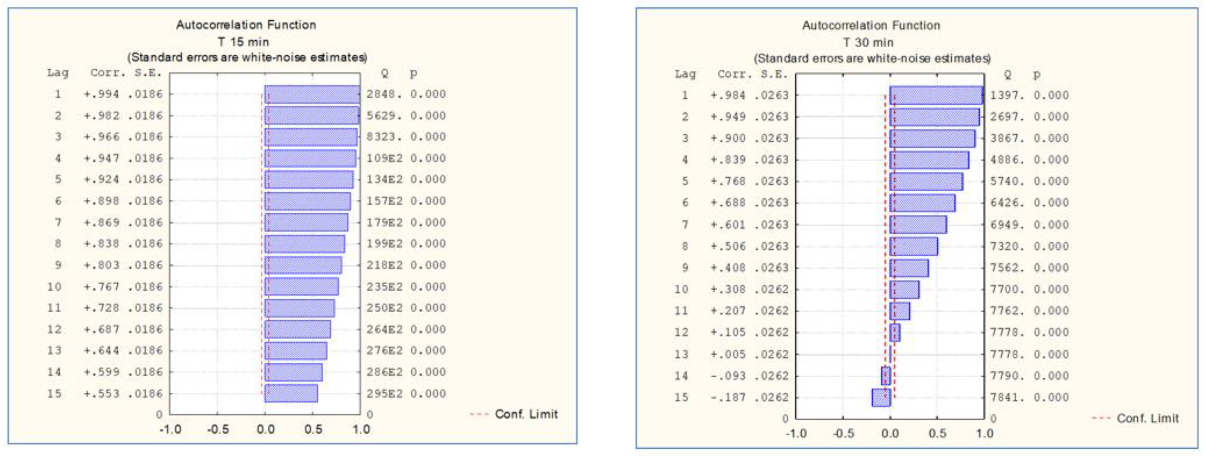
Figure 1. Autocorrelation functions LAG (15 min) and LAG (30 min) for air temperature.
Sustainability 15 02762 g001
Figure 2. Measurement units installed in C.R. ENEA, Casaccia.
Sustainability 15 02762 g002
Figure 3. Linear spline example of air temperature for one day and the residual values.
Sustainability 15 02762 g003
Figure 4. Minute-scale temperature estimations of the annual interval with the PSIHP function above and minute-scale measurements below.
Sustainability 15 02762 g004
Figure 5. Frequency distribution of the minute-scale temperature estimations of the annual interval with the PSIHP function above and frequency distribution of the minute-scale measurements below.
Sustainability 15 02762 g005
Figure 6. Comparison of the GHI trends (measurements and estimation using the Bourges physical model (red line) and cubic fitting (green line)) on a cloudy day (left; 11 January 2018) and on a clear sky day (right; 10 February 2018) for the location in Casaccia, Rome.
Sustainability 15 02762 g006
Figure 7. Schematic presentation of the “sinusoidal” empirical–statistical model interpolation and intra-hourly trends of S (solar data) in its time scale (H).
Sustainability 15 02762 g007
Figure 8. Comparison between the global horizontal irradiance trends of three different interpolation methods for a cloudy day (Casaccia, 11 January 2018).
Sustainability 15 02762 g008
Figure 9. Dispersion diagram of air temperature for the PCHIP interpolation and measurements (sampled data) for 2018.
Sustainability 15 02762 g009
Figure 10. Dispersion graph of the GHI using the “sinusoidal–physical model” interpolation for all cloud conditions.
Sustainability 15 02762 g010
Table 1. Statistical values of T, U and GHI.
Year 2018Temperature
(°C)
Specific Humidity(gwater vapor/kgair)Global Horizontal Irradiance (Only Daily Values) (W/m2)
Mean value16.788.61350.64
Standard error0.080.044.74
Median16.528.26277.2
St. deviation7.693.30289.98
Interval42.0216.951210
Min value−5.591.270
Max value36.4318.221210
Table 2. Clear sky and cloudy days observed in 2018, where 362 days with entire one-minute measurements were considered.
Type of SkyNumber of Days in 2018
kc < 0.65—cloudy242
Kc ≥ 0.65—clear sky120
Table 3. Synopsis of interpolation methods for solar irradiance.
Sub-Hourly Interpolation MethodsApplicability
Spline interpolation (PCHP)Clear sky
Physical model of Bourges with daily values of BClear sky
Physical model of Bourges with hourly B valuesClear sky
Sinusoidal–physical modelSky with any degree of cloudiness
Disclaimer/Publisher’s Note: The statements, opinions and data contained in all publications are solely those of the individual author(s) and contributor(s) and not of MDPI and/or the editor(s). MDPI and/or the editor(s) disclaim responsibility for any injury to people or property resulting from any ideas, methods, instructions or products referred to in the content.