Abstract
In the modern world, chronic kidney disease is one of the most severe diseases that negatively affects human life. It is becoming a growing problem in both developed and underdeveloped countries. An accurate and timely diagnosis of chronic kidney disease is vital in preventing and treating kidney failure. The diagnosis of chronic kidney disease through history has been considered unreliable in many respects. To classify healthy people and people with chronic kidney disease, non-invasive methods like machine learning models are reliable and efficient. In our current work, we predict chronic kidney disease using different machine learning models, including logistic, probit, random forest, decision tree, k-nearest neighbor, and support vector machine with four kernel functions (linear, Laplacian, Bessel, and radial basis kernels). The dataset is a record taken as a case–control study containing chronic kidney disease patients from district Buner, Khyber Pakhtunkhwa, Pakistan. To compare the models in terms of classification and accuracy, we calculated different performance measures, including accuracy, Brier score, sensitivity, Youdent, specificity, and F1 score. The Diebold and Mariano test of comparable prediction accuracy was also conducted to determine whether there is a substantial difference in the accuracy measures of different predictive models. As confirmed by the results, the support vector machine with the Laplace kernel function outperforms all other models, while the random forest is competitive.
1. Introduction
Chronic kidney disease (CKD) is a recognized priority of public health worldwide [1]. According to the 2010 Worldwide Burden Disease Study that listed the causes of mortality worldwide from 1990 to 2010, over two decades, CKD moved up on the list from the 27th to the 18th position [2]. Over the years, the epidemic of CKD has caused an 82% increase in years of life lost associated with kidney disease; a disease toll of the same magnitude as diabetes [3]. Premature death is part of the equation because most of the survivors of CKD move towards end-stage renal failure, a disability-related illness that reduces life quality and causes extensive social and financial losses. Although the annual patient rate of the incidence for renal replacement therapy (RRT) ranges dramatically across nations, varying from around 150 to 400 per million inhabitants (PMI) in the Western world to 50 PMIs or much less in developing countries, healthcare facilities are limited. Because early detection will help prevent the worsening of CKD and boost survivability, worldwide screening systems are being upgraded. Because of this, accurate epidemic-related knowledge of CKD at the national and international levels is very important in involving key stakeholders, such as patients, general practitioners, nephrologists, and financing organizations, who enable the healthcare system to plan and enforce effective preventive policies [4,5,6].
Nowadays, CKD is becoming an increasingly serious problem in both developed and developing countries. In developing countries, due to growing urbanization, people are adopting an unhealthy lifestyle, which causes diabetes and high blood pressure. The increasing urbanization in developing countries leads to chronic kidney disease, while 15–25% of people with diabetes die of kidney disease. For example, in Pakistan, CKD spreads quickly due to the ingestion of harmful and low-quality foods, self-medication, extreme use of drugs, polluted water, obesity, high blood pressure, hypertension, anemia, diabetes, and kidney stones [7]. However, in developed countries, such as the United States of America, 26 million adults (one in nine) have CKD, and other diseases are at a higher risk. USA researchers have developed an eight-point risk factor specification list to predict chronic kidney disease. The specification list includes older age, female sex, anemia, diabetes, hypertension, cardiovascular disease, and peripheral vascular disease [8]. According to recent studies, its prevalence ranges from 5–15% worldwide. Generally, around 5–10 million individuals die per year due to CKD [9]. As CKD worsens with time, detection and effective cures are simple curative ways of reducing the death rate.
Machine learning (ML) techniques play a prominent role in the medical sector for the identification of various diseases due to their specific features [10,11]. The authors of [12] used the support vector machine (SVM) approach to diagnose CKD. The authors used different kinds of data reduction techniques, i.e., principal component analysis (PCA). Their finding shows that the SVM model with Gaussian radial basis selection performed better in terms of diagnostic precision and accuracy than the rival models. Some researchers compared kernel functions based on random forest models. Few studies have compared computational intelligence and SVM models, others used artificial neural networks (ANN) and SVM algorithms to classify and predict four different types of kidney disease. According to the results, the ANN produced the most accurate results when compared to other models. Additionally, many researchers compared the statistical and computational intelligence models and the class-balanced order for dual classes of non-uniform distribution by featuring the ranks [13,14]. The authors of [15] showed in their investigation ways of detecting the appropriate diet plan for CKD patients, using many classification methods such as multiple class decision trees, multiple class decision forests, multiple class logistic regression, and multiple class ANN. The outcome shows that the multi-class decision forest achieved the highest accuracy (99.17%) in evaluation compared to the rest of the models.
Additionally, supervised classifier techniques are easy to use and have been widely applied in the diagnosis of various diseases in the past. The authors of [16] have used k-nearest neighbor (KNN) and SVM classifiers for the CKD dataset. For model comparison purposes, different types of performance measures like precision, recall, accuracy, and F1 score are considered. Based on the measures, KNN outperforms predicting CKD compared to SVM. The authors of [17] conducted a comparative analysis of ML and classical regression models, including artificial neural networks, decision trees, and logistic models, in terms of accuracy measures. After the comparison, it was shown that the highest accuracy (93%) was produced by ANN. In recent research, ML models were mostly used in the medical field. The authors of [18] utilized different kinds of ML methods, i.e., ANN, backpropagation, and SVM, for the classification and prediction of patients with kidney stone disease. Backpropagation is the best algorithm among all commonly used ML algorithms. On the other hand, some researchers compared naive Bayes (NB) models with the SVM algorithm. For example, the researchers in [19,20] used the NB models and SVM to identify different kinds of kidney disease and also check the accuracy of the models. In the end, the results specify that SVM models are more effective in classification and are considered the best classifiers. In this research, different ML models were used for comparative investigation for the prediction of CKD.
In this research study, various ML models were used for predicting CKD, and the main contributions are as follows:
- For the first time, we included primary data from CKD patients in district Buner, Kyber Pakhtunkhwa, Pakistan, to motivate developing countries to implement machine learning algorithms to reliably and efficiently classify healthy people and people with chronic kidney disease;
- To assess the consistency of the considered ML models, three different scenarios of training and testing set were adopted: (a) 90% training, 10% testing; (b) 75% training, 25% testing; and (c) 50% training, 50% testing. Additionally, within each validation scenario, the simulation was ran one thousand times to test the models’ consistency;
- The prominent machine learning models were used for the comparison of predicting CKD, including logistic, probit, random forest, decision tree, k-nearest neighbor, and support vector machine with four kernel functions (linear, Laplacian, Bessel, and radial basis kernels);
- The performance of the models is evaluated using the six performance measures, including accuracy, Brier score, sensitivity, Youdent, specificity, and F1 score. Moreover, to assess the significance of the differences in the prediction performance of the models, the Diebold and Mariano test was performed.
2. Materials and Methods
This section discusses in detail the considered predictive models, and the description of the features used in the kidney disease data of district Buner are discussed in detail.
2.1. Description of Variables
The dataset is collected from the Medical Complex, Buner Khyber Pakhtunkhwa, Pakistan. Diagnostic test reports have been observed for hundreds of patients on their arrival for a check-up with nephrologists at the Medical Complex, Buner, Khyber Pakhtunkhwa, Pakistan, with different twenty-one categorical variables illustrated in Table 1. These patients were observed from November 2020 to March 2021, and the sample size was calculated according to the formula in reference [21].

Table 1.
Description of variables.
Here, the sample size,, is the statistic with a subsequent level of confidence, is the expected prevalence proportion of CKD patients, , and m is the precision with a corresponding effect size. For the calculation of the expected sample size, we have assumed that 270 patients had CKD and 230 did not have CKD, and calculated the expected prevalence proportion , , (95% confidence interval), and ; some authors [22] recommended using 5% precision if the expected prevalence proportion lies between 10% and 90%. After putting the values of p, and in Equation (1), the approximated sample of size was produced, which is further used for analysis in this research.
2.2. Specification of Machine Learning Models
In this study, different ML predictive models were used, including logistic, probit, random forest, decision tree, k-nearest neighbor, and support vector machine with four kernel functions included (linear, Laplacian, Bessel, and radial basis kernels) models. Statistical software R version 3.5.3 was used in the analysis of data.
2.2.1. Logistic Regression (LR)
The LR model is a dominant and well-established supervised classification approach [23]. It is the extended form of the regression family and can be modeled as a binary variable, which commonly signifies the presence and absence of an event. It can be generalized to a multiple variable model, known as multiple logistic regression (MLR). The mathematical equation for MLR is
where are predictors. In our case, = 21 is thoroughly explained in the previews section. The unknown parameters are estimated by the MLE method.
2.2.2. K-Nearest Neighbor (KNN)
The KNN algorithm is one of the simplest and earliest classification algorithms [24]. It is used for the prediction of the label of a new data point based on its nearest neighbor labels in the training set if the new response is similar to the samples in the training part. Let be the training observations and the learning function , so that given an observation of , can determine the value.
2.2.3. Support Vector Machine (SVM)
SVM models are used to classify both linear and nonlinear data. They initially draw each data point into a variable space, with the number of variables k. Then, they use the hyperplane to divide the data items into two classes while maximizing the margin of distance for both classes and minimizing the error of classification [25]. The margin of the distance for a class is the distance between the nearest instance and the decision hyperplane, which is a member of that class. The SVM models use different kinds of functions that are known as the kernel. The kernel is used to transform data into the necessary form through input. The SVM models use different types of kernel functions. In this work, four kernels, linear, Laplacian, Bessel, and radial, are adopted as the basis.
Linear kernel: The linear kernel function is the modest one. These kernel functions return the inner product between two points in a suitable feature space.
Laplacian kernel: The Laplacian kernel function is completely correspondent to the exponential kernel, except for being less sensitive to changes in the sigma parameter.
Bessel kernel: The Bessel function is well-known in the theory of kernel function spaces of fractional smoothness, which is given as
where B is the Bessel function of the first kind.
Radial basis kernel: In SVM models, the radial basis, or RBF, is a popular kernel function used in various kernelized learning models.
2.2.4. Decision Tree (DT)
A DT is a tree-like structure, where each node indicates a feature, each branch indicates a decision rule, and each leaf represents a categorical or continuous value outcome. The main idea behind DT is to create a tree-like pattern for the overall dataset and process a single outcome at every leaf to reduce the errors in every leaf. DT separates observation into branches to make a tree improve prediction accuracy. In the DT algorithm, the identification of a variable and the subsequent cutoff for that variable breaks the input observation into multiple subsets by using mathematical techniques, i.e., information gain, Gini index, chi-squared test, etc. This splitting process is repeated until the construction of the complete tree. The purpose of splitting algorithms is to find the threshold for a variable that boosts up homogeneity in the output of samples. A decision tree is non-parametric and used to partition the data using some sort of mechanism to find the potential values in the feature [26]. In decision trees, the problem of overfitting is tackled by tuning hyper-parameters with the maximum depth and maximum leaf node of the tree. In our case, the hyper-parameters are tuned with maximum depths of 5, 10, 15, 20, 25, and 30 via an iterative process.
2.2.5. Random Forest (RF)
RF is a type of supervised ML algorithm. The name shows that it builds a forest, but it is made by some random. The decision trees grown very deep, frequently because of overfitting the training part, resulting in a great deviation in the outcome of classification for a slight variation in the input data. The different decision trees of the random forest are trained using the different training datasets. For the classification of a new sample, the input vector of that sample is needed to pass down each decision tree of the forest. Furthermore, each DT then considers a different part of that input vector and yields a classified outcome. The forest then opts for the classification of having the most ‘votes’ in case of discrete classification outcome, or the average of all trees in the forest in the form of a numeric classification outcome. Since the random forest algorithm considers the outcomes from many different decision trees, it can reduce the variation resulting from the consideration of a single decision tree for the same dataset [27].
2.3. Performance Measures
In this work, different performance measures are used for model comparison, such as accuracy, Brier score, sensitivity, Youdent, specificity, and F1 score.
2.3.1. Accuracy
The capacity of data items that is precisely classified is defined as accuracy. This means that the predictions of the data points are closer to the actual values. The mathematical equation can be described as
2.3.2. Brier Score
Brier Score (BS) is identified by the difference between the summation of the mean squared predicted probabilities and the observed binary output. The mathematical formula can be described as
Here, r shows the predicted probability in the category, and is the related observed binary output with probability in the category of classification. The minimum value of BS shows that the method is consistent and accurate.
2.3.3. Sensitivity
The measure of true positive observations that are properly identified as positive is called sensitivity. The mathematical formula is
2.3.4. Youdent
Youdent can be generally described as . The cut-point that attains this high is decribed as the optimum cut-point since it is the cut-point that improves the biomarker’s distinguishing capability when equivalent weight is given to specificity and sensitivity.
2.3.5. Specificity
The quantity of true negative values that are precisely recognized as negative is called specificity. The mathematical formula is
2.3.6. F1 Score
The amount of mixture of precision and recall to retain stability between Them is called F1 score
The mathematical function for computing the F1 score is given by
F1 score confirmed the goodness of classifiers in the terms of precision or recall.
3. Results and Discussion
This section elaborates on the results from different perceptions. Initially, we investigate the performance of various machine learning methods, such as LR, PB, KNN, DT, RF, SVM-L, SVM-LAP, SVM-RB, and SVM-B, on the CKD dataset. For the training and testing prediction, consider three different scenarios, including 50%, 75%, and 90%. To evaluate the prediction performance of the selected models, six performance measures were used, namely, accuracy, Brier score, sensitivity, Youdent, specificity, and F1 score, for each method for a total of one thousand runs.
In the initial scenario, the training dataset is 90% and the testing is 10%. The results are shown in Table 2. In Table 2, it is evident that the SVM-LAP and RF produce better predictions as compared to the rest of the models. The best predictive model obtained 0.9171, 0.8671, 0.9484, 0.8155, 0.0643, 0.0829, and 0.9319 for mean accuracy, specificity, sensitivity, Youdent, Brier score, F1 score, and error, respectively. RF produced the second best results compared to the other models, while LG and PB performed better than the remaining two models. We can also check the superiority of models by creating figures. For example, Figure 1 shows the mean accuracy, Brier score, sensitivity, Youdent, specificity, and F1 score of all the models. As seen from all figures, the SVM-Lap produces superior outcomes compared to the rest of the models. Although RF is competitive, KNN showed the worst results.
Table 2.
First scenario (90%, 10%): different performance measures and row-wise predictive models in rows.
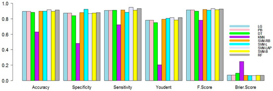
Figure 1.
Performance measure plots (90% training, 10% testing) of the models.
In the second scenario, the training dataset is 75% and testing is 25%. The results are shown in Table 3. In Table 3, it is evident again that SVM-Lap and RF led to a better prediction than the competitor predictive models. The best predictive model produced 0.9135, 0.8643, 0.9468, 0.8111, 0.0663, 0.0865, and 0.9328 for mean accuracy, specificity, sensitivity, Youdent, Brier-score, F1 score, and error, respectively. RF again produced the second best results. The superiority of the model can be observed in the figures. For example, Figure 2 shows the mean accuracy, specificity, sensitivity, Youdent, Brier score, and F1 score of all models. As seen from all figures, SVM-Lap produces superior results compared to the rest of the models. Although RF is competitive and KNN shows the worst results compared to the rest.
Table 3.
Second scenario (75%, 25%): different performance measures and row-wise predictive models in rows.
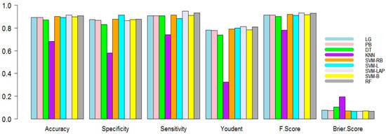
Figure 2.
Performance measure plots (50% training, 50% testing) of the models.
Finally, in the third scenario, the training dataset is 50% and the testing is 50%. The outcomes are listed in Table 4. As seen in Table 4, it is evident again that SVM-Lap and RF have a better prediction. This time, the best predictive model produced 0.9052, 0.8585, 0.9449, 0.8034, 0.0701, 0.0948, and 0.9304 for mean accuracy, specificity, sensitivity, Youdent, Brier score, F1 score, and error, respectively. RF again produced the second best results. The superiority of the model is shown in the figures. For example, Figure 3 shows the mean accuracy, specificity, sensitivity, Youdent, Brier score, and F1 score of all models. It conforms to all other figures; SVM-Lap produces the lowest error. Although RF is competitive, KNN shows the worst results compared to all the models.
Table 4.
Third scenario (50%, 50%): different performance measures and row-wise predictive models in rows.
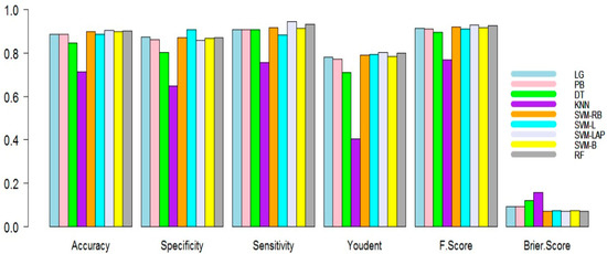
Figure 3.
Performance measure plots (75% training, 25% testing) of the models.
Once the accuracy measures were computed, the superiority of these results was evaluated. For this purpose, in the past, many researchers performed the Diebold and Mariano (DM) test [28,29,30]. In this study, to verify the superiority of the predictive model results (accuracy measures) listed in Table 2, Table 3 and Table 4, we used the DM test [31]. A DM test is the most used statistical test for comparative predictions acquired from different models. The DM test for identical prediction accuracy has been performed for pairs of models. The results (p-values) of the DM test are listed in Table 5; each entry in the table shows the p-value of a hypothesis assumed, where the null hypothesis supposes no difference in the accuracy of the predictor in the column or row against the research hypothesis that the predictor in the column is more accurate as compared to the predictor in the row. In Table 5, we observed that the prediction accuracy of the previously defined model is not statistically different from all other models except for KNN.
Table 5.
p-values for the Diebold and Marion test identical prediction accuracy against the alternative hypothesis that the model in the column is more accurate than in the row (using squared loss function).
In the end, we also plotted an error box plot for each scenario with all predictive models. This error was obtained as (1-accuracy), during the one thousand simulations for model consistency. It can see in Figure 4a that the first scenario is 90%, 10%; in Figure 4b, the second scenario is 75%, 25%, and in Figure 4c the third scenario is 50%, 50%. In all three cases, SVM-LAP captures the lowest variation, and the second best model is RF. Additionally, confirmed in Figure 4a–c, KNN produces the worst results. Finally, it is confirmed that SVM-LAP is highly efficient for the prediction of CKD in patients, and RF is the second best model.
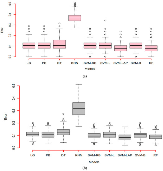
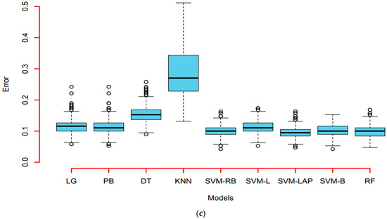
Figure 4.
(a) Error box-plots (90% training, 10% testing) of the models; (b) Error box-plots (50% training, 50% testing) of the models; (c) Error box-plots (75% training, 25% testing) of the models.
4. Conclusions
In this research, we attempted a comparative analysis of different machine learning methods using the CKD data of district Buner, Khyber Pakhtunkhwa, Pakistan. The dataset consists of records collected as part of a case–control study involving patients with CKD from the entire Buner district. For the training and testing prediction, we considered three different scenarios, including 50%, 75%, and 90%. For the comparison of the models in terms of classification, we calculated various performance measures, i.e., accuracy, Brier score, sensitivity, Youdent, specificity, and F1 score. The results indicate that the SVM-LAP model outperforms other models in all three scenarios, while the RF model is competitive. Additionally, the DM test was used to ensure the superiority of predictive model accuracy measures. The result (DM test p-values) shows the best performance of all used methods in the prediction of chronic kidney disease, excluding the KNN method.
This study can be further extended in future research projects in medical sciences by, for example, predicting the effectiveness of a particular medicine in specific diseases. Furthermore, the reported best ML models in this work can be used to predict other conditions, such as heart disease, cancer, and tuberculosis. Moreover, a novel hybrid system for the same dataset will be proposed to obtain more accurate and efficient prediction results.
Author Contributions
H.I., conceptualized and analyzed the data, and prepared the figures and draft; M.K., collect data, designed the methodology, performed the computation work, prepared the tables and graphs, and authored the draft; Z.K., supervised, authored, reviewed, and approved the final draft; F.K., H.M.A. and Z.A. authored, reviewed, administered, and approved the final draft. All authors have read and agreed to the published version of the manuscript.
Funding
Princess Nourah bint Abdulrahman University Researchers Supporting Project number (PNURSP2023R 299), Princess Nourah bint Abdulrahman University, Riyadh, Saudi Arabia.
Informed Consent Statement
Informed consent was obtained from all subjects involved in the study.
Data Availability Statement
The research data will be provided upon the request to the first author.
Acknowledgments
Princess Nourah bint Abdulrahman University Researchers Supporting Project number (PNURSP2023R 299), Princess Nourah bint Abdulrahman University, Riyadh, Saudi Arabia.
Conflicts of Interest
The authors declare no conflict of interest.
References
- Yan, M.T.; Chao, C.T.; Lin, S.H. Chronic kidney disease: Strategies to retard progression. Int. J. Mol. Sci. 2021, 22, 10084. [Google Scholar] [CrossRef] [PubMed]
- Lozano, R.; Naghavi, M.; Foreman, K.; Lim, S.; Shibuya, K.; Aboyans, V.; Abraham, J.; Adair, T.; Aggarwal, R.; Ahn, S.Y.; et al. Global and regional mortality from 235 causes of death for 20 age groups in 1990 and 2010: A systematic analysis for the Global Burden of Disease Study 2010. Lancet 2012, 380, 2095–2128. [Google Scholar] [CrossRef]
- Jha, V.; Garcia-Garcia, G.; Iseki, K.; Li, Z.; Naicker, S.; Plattner, B.; Saran, R.; Wang, A.Y.M.; Yang, C.W. Chronic kidney disease: Global dimension and perspectives. Lancet 2013, 382, 260–272. [Google Scholar] [CrossRef] [PubMed]
- Eckardt, K.U.; Coresh, J.; Devuyst, O.; Johnson, R.J.; Köttgen, A.; Levey, A.S.; Levin, A. Evolving importance of kidney disease: From subspecialty to global health burden. Lancet 2013, 382, 158–169. [Google Scholar] [CrossRef]
- Rapa, S.F.; Di Iorio, B.R.; Campiglia, P.; Heidland, A.; Marzocco, S. Inflammation and oxidative stress in chronic kidney disease—Potential therapeutic role of minerals, vitamins and plant-derived metabolites. Int. J. Mol. Sci. 2019, 21, 263. [Google Scholar] [CrossRef]
- Jayasumana, C.; Gunatilake, S.; Senanayake, P. Glyphosate, hard water and nephrotoxic metals: Are they the culprits behind the epidemic of chronic kidney disease of unknown etiology in Sri Lanka? Int. J. Environ. Res. Public Health 2014, 11, 2125–2147. [Google Scholar] [CrossRef] [PubMed]
- Mubarik, S.; Malik, S.S.; Mubarak, R.; Gilani, M.; Masood, N. Hypertension associated risk factors in Pakistan: A multifactorial case-control study. J. Pak. Med. Assoc. 2019, 69, 1070–1073. [Google Scholar]
- Naqvi, A.A.; Hassali, M.A.; Aftab, M.T. Epidemiology of rheumatoid arthritis, clinical aspects and socio-economic determinants in Pakistani patients: A systematic review and meta-analysis. JPMA J. Pak. Med. Assoc. 2019, 69, 389–398. [Google Scholar]
- Hsu, R.K.; Powe, N.R. Recent trends in the prevalence of chronic kidney disease: Not the same old song. Curr. Opin. Nephrol. Hypertens. 2017, 26, 187–196. [Google Scholar] [CrossRef]
- Salazar, L.H.A.; Leithardt, V.R.; Parreira, W.D.; da Rocha Fernandes, A.M.; Barbosa, J.L.V.; Correia, S.D. Application of machine learning techniques to predict a patient’s no-show in the healthcare sector. Future Internet 2022, 14, 3. [Google Scholar] [CrossRef]
- Elsheikh, A.H.; Saba, A.I.; Panchal, H.; Shanmugan, S.; Alsaleh, N.A.; Ahmadein, M. Artificial intelligence for forecasting the prevalence of COVID-19 pandemic: An overview. Healthcare 2021, 9, 1614. [Google Scholar] [CrossRef] [PubMed]
- Khamparia, A.; Pandey, B. A novel integrated principal component analysis and support vector machines-based diagnostic system for detection of chronic kidney disease. Int. J. Data Anal. Tech. Strateg. 2020, 12, 99–113. [Google Scholar] [CrossRef]
- Zhao, Y.; Zhang, Y. Comparison of decision tree methods for finding active objects. Adv. Space Res. 2008, 41, 1955–1959. [Google Scholar] [CrossRef]
- Vijayarani, S.; Dhayanand, S.; Phil, M. Kidney disease prediction using SVM and ANN algorithms. Int. J. Comput. Bus. Res. (IJCBR) 2015, 6, 1–12. [Google Scholar]
- Dritsas, E.; Trigka, M. Machine learning techniques for chronic kidney disease risk prediction. Big Data Cogn. Comput. 2022, 6, 98. [Google Scholar] [CrossRef]
- Wickramasinghe, M.P.N.M.; Perera, D.M.; Kahandawaarachchi, K.A.D.C.P. (2017, December). Dietary prediction for patients with Chronic Kidney Disease (CKD) by considering blood potassium level using machine learning algorithms. In Proceedings of the 2017 IEEE Life Sciences Conference (LSC), Sydney, Australia, 13–15 December 2017; IEEE: Piscataway, NJ, USA, 2018; pp. 300–303.
- Gupta, A.; Eysenbach, B.; Finn, C.; Levine, S. Unsupervised meta-learning for reinforcement learning. arXiv 2018, arXiv:1806.04640. [Google Scholar]
- Lakshmi, K.; Nagesh, Y.; Krishna, M.V. Performance comparison of three data mining techniques for predicting kidney dialysis survivability. Int. J. Adv. Eng. Technol. 2014, 7, 242. [Google Scholar]
- Zhang, H.; Hung, C.L.; Chu, W.C.C.; Chiu, P.F.; Tang, C.Y. Chronic kidney disease survival prediction with artificial neural networks. In Proceedings of the 2018 IEEE International Conference on Bioinformatics and Biomedicine (BIBM), Madrid, Spain, 3–6 December 2018; IEEE: Piscataway, NJ, USA, 2018; pp. 1351–1356. [Google Scholar]
- Kavakiotis, I.; Tsave, O.; Salifoglou, A.; Maglaveras, N.; Vlahavas, I.; Chouvarda, I. Machine learning and data mining methods in diabetes research. Comput. Struct. Biotechnol. J. 2017, 15, 104–116. [Google Scholar] [CrossRef]
- Singh, V.; Asari, V.K.; Rajasekaran, R. A Deep Neural Network for Early Detection and Prediction of Chronic Kidney Disease. Diagnostics 2022, 12, 116. [Google Scholar] [CrossRef]
- Pourhoseingholi, M.A.; Vahedi, M.; Rahimzadeh, M. Sample size calculation in medical studies. Gastroenterol. Hepatol. Bed Bench 2013, 6, 14. [Google Scholar]
- Naing, L.; Winn TB, N.R.; Rusli, B.N. Practical issues in calculating the sample size for prevalence studies. Arch. Orofac. Sci. 2006, 1, 9–14. [Google Scholar]
- Nhu, V.H.; Shirzadi, A.; Shahabi, H.; Singh, S.K.; Al-Ansari, N.; Clague, J.J.; Jaafari, A.; Chen, W.; Miraki, S.; Dou, J.; et al. Shallow landslide susceptibility mapping: A comparison between logistic model tree, logistic regression, naïve bayes tree, artificial neural network, and support vector machine algorithms. Int. J. Environ. Res. Public Health 2020, 17, 2749. [Google Scholar] [CrossRef] [PubMed]
- Joachims, T. Making large-scale svm learning. In Practical Advances in Kernel Methods-Support Vector Learning; MIT Press: Cambridge, MA, USA, 1999. [Google Scholar]
- Criminisi, A.; Shotton, J.; Konukoglu, E. Decision forests: A unified framework for classification, regression, density estimation, manifold learning and semi-supervised learning. Found. Trends Comput. Graph. Vis. 2012, 7, 81–227. [Google Scholar] [CrossRef]
- Tyralis, H.; Papacharalampous, G.; Langousis, A. A brief review of random forests for water scientists and practitioners and their recent history in water resources. Water 2019, 11, 910. [Google Scholar] [CrossRef]
- Shah, I.; Iftikhar, H.; Ali, S.; Wang, D. Short-term electricity demand forecasting using components estimation technique. Energies 2019, 12, 2532. [Google Scholar] [CrossRef]
- Shah, I.; Iftikhar, H.; Ali, S. Modeling and forecasting medium-term electricity consumption using component estimation technique. Forecasting 2020, 2, 163–179. [Google Scholar] [CrossRef]
- Shah, I.; Iftikhar, H.; Ali, S. Modeling and forecasting electricity demand and prices: A comparison of alternative approaches. J. Math. 2022, 2022. [Google Scholar] [CrossRef]
- Diebold, F.X.; Mariano, R.S. Comparing predictive accuracy. J. Bus. Econ. Stat. 2002, 20, 134–144. [Google Scholar] [CrossRef]
Disclaimer/Publisher’s Note: The statements, opinions and data contained in all publications are solely those of the individual author(s) and contributor(s) and not of MDPI and/or the editor(s). MDPI and/or the editor(s) disclaim responsibility for any injury to people or property resulting from any ideas, methods, instructions or products referred to in the content. |
© 2023 by the authors. Licensee MDPI, Basel, Switzerland. This article is an open access article distributed under the terms and conditions of the Creative Commons Attribution (CC BY) license (https://creativecommons.org/licenses/by/4.0/).