Systemic Risk with Multi-Channel Risk Contagion in the Interbank Market

Abstract

The systematicness of banks is an important driver of financial crisis. Overlapping portfolios and assets correlation of banks’ investment are important reasons for systemic risk contagion. The existing systemic risk models are all analyzed from one aspect and cannot reflect the real situation of the banking system. In the present paper, considering the overlapping portfolios and assets correlation, a contagion network model with multi-channel risk is proposed, which is with interbank lending (direct contagion channel), overlapping portfolios (indirect contagion channel), and assets correlation (indirect contagion channel). In addition, the model takes investment risk as an impact factor and learns the operation rules of the banking system to help banks compensate for liquidity through asset depreciation. Based on the proposed model, the effects of assets correlation, assets diversity, assets investment strategy, interbank network structure, and the impact of market density on risk contagion are studied and analyzed quantitatively. The method in this paper can more truly reflect the banking system risk than the existing model. This paper provides a solution for quantitative analysis of systemic risk, which provides powerful tools for macroprudential stress testing and a reference for regulatory authorities to prevent systemic risk.

1. Introduction

The recent financial crisis has had a huge impact on world finance. For example, the financial crisis in 2008 led to a large number of bankruptcies of American banks and European banks. In the nine years after the collapse of Lehman Brothers, the combined benefits of the European debt crisis led to a sharp decline of 25% in the number of European banks. Studies on the impact on financial network systems, which financial network systems are subject to systemic risk [1,2,3,4]. Systemic risk refers to the total or partial damage of the financial system, resulting in the destruction of financial services or functions. From the perspective of risk contagion, systemic risk refers to the possibility of asset loss of a single institution, resulting in the transmission of individual financial risks to the entire market and causing domino effect. In fact, systemic risk prevention is an important part of economic sustainability, and systemic risk analysis is the premise of systemic risk prevention. Therefore, the analysis of systemic risk is an important aspect of economic sustainability. A complicated network system made up of numerous banks and their connections is known as a banking network system. In addition to being directly tied to the interbank market, the ties are also implicitly linked to banks investing in equivalent assets. Currently, the majority of studies on systemic risk examine the risk of banking network systems from the perspective of the interbank market (direct channel) [5,6,7]. The interbank market helps banks make up for lack of liquidity and offers contagious pathways for the crisis’ spread [8,9,10]. The interbank market is crucial for reducing systemic risk [11,12,13]. The interbank market can cope with the impact of liquidity risk, but it also served as a risk contagion route for bank collapse, according to Mistrulli’s empirical analysis [14]. Allen and Gale [15] discovered that market structure significantly affects the likelihood of Risk Shocks in the interbank market, with the complete market structure being more resilient than the incomplete market. Similar to Allen’s research [15], Freixas and Rochet [16] discovered that the stronger the connections between banks, the quicker each bank recovered throughout the crisis. Leitner [17] investigated the ideal structure of a banking network system and discovered that it should strike a balance between risk sharing and probable “domino collapse”. To investigate the effects of homogeneous banks and heterogeneous banks on the stability of banking network systems when banks’ investment behavior is regulated, Iori et al. [18]. built a stochastic interbank network model. According to Nier et al. [19], the effect of interbank links on systemic risk is not constant. At first, a little increase in connections led to an increase in infection. When connectivity reaches a particular level, connectivity boosts the financial network system’s capacity to withstand shocks, hence enhancing its stability. May and Arinaminpathy [20] studied the interaction between the characteristics of a single bank and the overall dynamic behavior of the system. Caccioli et al. [21] obtained a leverage threshold, which made it difficult for financial institutions to liquidity in risky markets and was likely to fail. On the basis of the interbank market, Gabbi et al. [22] combined the real economy and the central bank and analyzed the effects of various network organization on the balance of the banking network system and the trade-off between economic gains. Xu et al. [23] established a dynamic banking network model based on bank director behaviors to evaluate the financial contagion of counterparties and liquidity channels in the interbank market. From a cross-sectional perspective, Laeven and Ratnovski [24] examined the features of risk contagion induced by a Single Bank and discovered that large-scale and low-capital institutions can raise systemic risk. Gai and Kapadia [25] discussed how aggregate and special shocks, changes in network structure, and asset market liquidity affect contagion. He found that although the probability of infection was low, but once the infection occured, it would be very serious. Fan and Li [26] built a multi-agent dynamic banking network model and discovered that unrestrained investment activity will make the banking network system more unstable. Kok [27] presented a continuous network building mechanism to investigate how the interbank network structure is impacted by the major parameters. Han and Yu [28] discovered that while risk aversion boosted systemic risk contagion, liquidity hoarding reduced systemic risk in the early stages. A network-based credit risk structure model was created by Steinbacher et al. [29]. To illustrate how particular and systemic shocks propagated throughout the banking network system.

Most of existing studies are based on the direct related risk contagion in the interbank market, but few studies have been conducted on the indirect related risk contagion caused by the overlapping portfolios invested by banks. Furthermore, a growing number of academics think that the indirect relationship between banks [30,31,32,33,34,35] has a larger role in the likelihood of risk contagion than the direct concact based on The Inter-Bank Market [36]. According to Lagunoff [37], one key factor in the propagation of systemic risk is the overlap in bank portfolios. Uhlig [38] investigated two different financial crises using overlapping portfolios. One type was the redistribution of portfolios by banks as a result of outside shocks. In this instance, the financial crisis was brought on by the slow increase of asset losses, which had stressed more bank assets. Another type was when certain banks moved their means to safer portfolio management, which led to a decline in means prices and crises. Caccioli et al. [39] discussed the influence of overlapping portfolios on risk contagion. The results show that the excessive diversification of investment will lead to a closer coupling relationship between banks and make financial contagion more serious. Vries [40] conducted a research similar to Uhlig’s work. Because of the correlation of banks’ assets, the ’fat tail’ of banks’ assets distribution brings bankruptcy risk to banks. Huang et al. [41] constructed a bank-asset bipartite network model and used 2007 balance sheet data of American commercial banks to study the risk of contagion empirically. Caccioli et al. [42] constructed a multi-assets model of investment, and discussed the probability and extent of financial contagion under different conditions of leverage, market congestion, and assets diversity. Rodrigo et al. [43] found that the asset sales of troubled institutions depressed the market price of these assets. Small scale shocks can lead to risk contagion. Greenwood et al. [44] found that the risk contagion mainly came from the decline in assets prices in the network with overlapping portfolios. Tasca et al. [45] revealed that the systemic risk can be contagious through the assets networks held by banks.

The research mentioned above mostly examine systemic risk from the standpoint of overlapping portfolios or interbank lending, but they do not combine asset portfolios with interbank lending or thoroughly study the interbank network’s evolution law with assets coupling. Asset coupling refers to the correlation between different assets. The change of one asset price will cause the change of another asset price. Asset coupling is different from overlapping portfolios, overlapping portfolios means that banks holding the same assets. A complicated network architecture that took into account interbank lending and overlapping portfolios was proposed by Zhou and Li [46]. However, Zhou’s work has fixed capital asset ratios, fixed interbank lending ratios, and unclear investment and lending techniques. Moreover, the current researches on the overlapping portfolios of banks mainly considered the risk contagion caused by the same assets among banks, but did not consider the correlation between assets. Current research lacks the correlation analysis between invested assets, which leads to the result that the probability and degree of risk contagion caused by indirect infection are likely to be underestimated or miscalculated [47]. Many researches investigated that the correlation between assets was an indirect channel of credit risk contagion [48]. However, how assets correlation affects systemic risk in the interbank network is not clear, which requires the establishment of a mechanism model for analysis. Furthermore, there are some issues with the preceding work. For example, the yield of asset investment generally fluctuates at a fixed value, but there are risks in the market, and the yield will fluctuate greatly. In most models, banks cannot supplement the flow of funds by selling or converting assets, which is inconsistent with the laws of financial markets.

Based on the above research, a multi-scale systemic risk prediction model of interbank network system is constructed. According to the model, the overlapping portfolios (indirect contagion channel) and the interbank lending (direct contagion channel) are considered for the systemic risk. In addition, the model also considers the correlation between different assets (indirect contagion channel). Banks can improve liquidity through a variety of means, including inter-bank loans and asset sales. When selling assets, banks also consider the depreciation of assets held by each other, while considering changes in assets prices caused by the coupling relationship between assets. According to the proposed model, the average return of investment held by banks is dynamic and can vary with the change of economic conditions. The proposed method is discussed from three perspectives: the systemic risk index, average probability of risk contagion, and the average degree of the risk contagion. The dynamic change in the systemic risk of the banking network system over time can be reflected by the systemic risk index. The risk contagion of the banking network system is statistically analyzed using the average probability of the risk contagion and the average degree of the risk contagion. This paper explores the impact of assets correlation, assets diversity, assets investment strategy, interbank network structure, and market density on the banking network system in order to better understand the systemic risk contagion mechanism.

2. Multi-Channel Risk Contagion Model

Bank failures are frequently caused by a lack of liquidity in a banking network system. Bank liquidity is closely related to deposits, investments, and interbank borrowing. Figure 1 depicts the construction of a multi-channel risk contagion model of banking network system. In this model, we consider the impact of interbank lending (direct contagion channel), overlapping portfolios (indirect contagion channel) and assets correlation (indirect contagion channel) on the systemic risk, which can better reflect the actual regulations of the banking network system. For example, through systematic analysis, policy makers can effectively regulate the financial market by means of interest rate adjustment, deposit reserve ratio adjustment.

2.1. A Dynamic Banking Network System with Interbank Lending

Banks can borrow funds from interbank markets when they lack liquidity, as illustrated in Figure 1. In the banking network system, the possible lending relationship among banks is expressed by the connection matrix J, where $J_{ij}$ is 1 or 0. $J_{ij}=1$ indicates the possible credit connection between bank i and bank j, while $J_{ij}=0$ indicates that bank i and bank j have no lending relationship with each other. Possible credit connections between bank i and bank j are generated by probabilistic $p_{ij}$ $(0\le p_{ij}\le 1)$. A bank will only borrow from some banks, not from all banks without purpose. Bank i may borrow from bank j, but it must satisfy $J_{ij}=1$. The choice of lender is determined by the bank’s preference. The preference indicates that each bank has some preferred partners. Within a certain period, the bank’s lending preference is assumed to remain unchanged. When bank i requires interbank borrowing, it will borrow from the banks with $J_{ij}=1$ at random. $N_t$ indicates the number of banks at time t. $N_t$ indicates a bounded integer. The dynamic banking network system changes throughout discrete time t, $t=1,2,3,\dots ,T$. The bank i’s liquidity at time t can be described as [18]:

$$L_i\left(t\right)={\widehat{L}}_i\left(t\right)-D_i\left(t\right)-I_i\left(t\right)+\sum _{j=1}^{N_t}{c}_{ij}\left(t\right)B_{ij}\left(t\right),$$

(1)

where ${\widehat{L}}_i\left(t\right)$ indicates the bank i’s liquidity assets prior to investment, dividend, and lending. $D_i\left(t\right)$ indicates bank i’s dividend at time t. $I_i\left(t\right)$ indicates bank i’s investment at time t. $c_{ij}$ describes the lending connection between bank i and bank j. If bank i and bank j are lending to one another, $c_{ij}=1$, otherwise $c_{ij}=0$ ($c_{ij}$ ≠ $J_{ij}$. $c_{ij}$ denotes the actual loan relationship between bank i and bank j, while $J_{ij}$ denotes the possible credit relationship between two banks). $B_{ij}\left(t\right)>0$ means the amount borrowed by bank i from bank j. $B_{ij}\left(t\right)<0$ means bank j loans to bank i, and $B_{ij}\left(t\right)=-B_{ji}\left(t\right)$.

At each time t, deposits will change, banks need to pay interest on previous deposits, and banks can obtain the return of investment, which leads to changes in banks’ liquidity. Bank i’s liquidity prior to investment, dividends, and borrowing at time t can be described as:

$${\widehat{L}}_i\left(t\right)=L_i(t-1)+A_i\left(t\right)-A_i(t-1)-r_a{A}_i(t-1)+U_i\left(t\right),$$

(2)

where $A_i\left(t\right)$ denotes the deposits held by bank i at time t, $r_a$ denotes the interest rate of bank deposits and $U_i\left(t\right)$ denotes the investment recovery of bank i. In practice, the depositor’s deposit behavior is random, so bank i’s deposit at time t is:

$$A_i\left(t\right)=(1+{\sigma }_A{\eta }_t)\widehat{A},$$

(3)

where ${\sigma }_A$ denotes the standard deviation of all banks’ random deposits, $\overline{A}$ denotes the mean of all banks’ deposits, ${\eta }_t\in N(0,1)$. The following are all of the investment assets that bank i possessed at t time without investment:

$$Y_i\left(t\right)=\sum _{k=1}^M{Q}_{ik}\left(t\right)g_k\left(t\right),$$

(4)

where $Q_{ik}\left(t\right)$ represents the amount of shares of assets k that bank i owns at time t. $Q_{ik}\left(t\right)$ is a dynamic change value since bank i may make new investments and there may be asset liquidation at each time step. $g_k\left(t\right)$ represents asset k’s price at time t, and it can be expressed as follows:

$$g_k\left(t\right)=g_k(t-1)(1+{\delta }_k\left(t\right)),$$

(5)

where ${\delta }_k\left(t\right)$ represents the return rate on investment k at time t. The return rate on investment k is stochastic, and ${\delta }_k\left(t\right)$ follows the normal distribution with mean $\tau$, namely ${\delta }_k\left(t\right)\in N(\tau ,\theta )$. $\tau$ can be regarded as the average return rate with regard to all investments. $\theta$ indicates asset prices’ volatility. At time t, banks will partially recoup their investment assets $U_i\left(t\right)=q\times Y_i\left(t\right)$, where q represents the percentage of investment recovery. Following investment recovery, all investment assets bank i owns prior to continued investment are ${\widehat{Y}}_i\left(t\right)={\displaystyle \sum _{k=1}^M}{\widehat{Q}}_{ik}\left(t\right)g_k\left(t\right)$. ${\widehat{Q}}_{ik}\left(t\right)$ indicates the amount of assets k’s shares retained by bank i after investment recovery. When a bank gets enough investment profit, it will pay dividends. Bank i’s dividends $D_i\left(t\right)$ at time t can be described as:

$$\begin{array}{cc}\hfill D_i\left(t\right)=& max\{0,min[U_i\left(t\right)-r_a{A}_i(t-1),{\widehat{L}}_i\left(t\right)-\beta A_i\left(t\right),\hfill \\ \hfill & {\widehat{L}}_i\left(t\right)+{\widehat{Y}}_i\left(t\right)-(1+\chi )A_i\left(t\right)\left]\right\},\hfill \end{array}$$

(6)

where $\chi$ represents the capital savings ratio, and $\beta$ represents the deposit reserve ratio. Bank’s dividends need to be met: ${\widehat{V}}_i\left(t\right)/A_i\left(t\right)\ge \chi$. ${\widehat{V}}_i\left(t\right)$ denotes the owner’s equity of bank i before dividends and investments at time t, which is calculated as:

$${\widehat{V}}_i\left(t\right)={\widehat{L}}_i\left(t\right)+{\widehat{Y}}_i\left(t\right)-A_i\left(t\right)-(1+r_b)B_i(t-1).$$

(7)

When the dividend is paid, the bank needs to reinvest it, and the investment needs to satisfy the requirements of existing liquidity funds and stochastic investment opportunities:

$$I_i\left(t\right)=min\{max[0,{\widehat{L}}_i\left(t\right)-\beta A_i\left(t\right)-D_i\left(t\right)],w_i\left(t\right)\},$$

(8)

where $w_i\left(t\right)$ denotes bank i’s investment opportunity at time t, which is defined as follows:

$$w_i\left(t\right)=\overline{w}(1+{\sigma }_w\mu ),$$

(9)

where $\overline{w}$ denotes the average of all banks’ investment opportunities. ${\sigma }_w$ denotes the standard deviation of all banks’ investment opportunities. $\mu$ follows the normal distribution $N(0,1)$. Suppose the amount of assets k bank i invests at time t is $▵Q_{ik}\left(t\right)$. Thus, the entire amount of assets k bank i invests is $Q_{ik}\left(t\right)=▵Q_{ik}\left(t\right)+{\widehat{Q}}_{ik}\left(t\right)$. Following investment, the value of $Y_i\left(t\right)$ is updated to $Y_i\left(t\right)={\displaystyle \sum _{k=1}^M}{Q}_{ik}\left(t\right)g_k\left(t\right)$. In this work, the bank-asset network is also a random network. The rule of bank holding assets is: when bank i invests, the link probability between bank and asset is set to 0.01 in this work. To ensure that the number of assets invested in each investment is limited. In fact, in the real banking system, the average number of assets held by each bank is not fixed. This value refers to the average number of assets held by banks in the real banking system [42]. About 0.01 M assets are invested by bank i, and the total amount of these assets invested is generated randomly, but the total amount of all invested assets is equivalent to the total amount of investment the bank needs to invest.

In the above-mentioned banking system, the following bankruptcies occur: insufficient liquidity, unable to pay off debts, or unable to pay deposits interest. After a bank pays dividends and invests, if there is surplus liquidity capital. This bank is a prospective creditor bank, that could break up funding in the interbank market. To operate normally, indebted banks need to loan money from the interbank market. With regard to a debtor bank, if sufficient funds are available from the interbank market to pay off the loan and interest for the previous period, the repayment will be made. Simultaneously, the debt banks’ liquidity falls to zero. If a bank cannot borrow money, or borrow insufficiently to repay deposit interest and loans, the debt bank will vend investment assets until they can pay off deposit interest and loans. If the proceeds from the sale of assets are insufficient to pay out the prior deposits interest and loans, the debtor’s bank will fail and liquidate the assets. The assets must be used to pay off deposits first, with the remainder paid pro rata to creditor banks, and then the liquidity of each bank should be recalculated.

2.2. Overlapping Portfolios and Asset Correlation

As shown in Figure 1, the banking network is a network indirectly linked by overlapping portfolios. Suppose there are N banks and millions of dollars in assets within the network, and the market density is expressed as $MD=frackMN$. Each bank invests in accordance with Equation (8), bank i’s portfolio is $\{H_{i1},H_{i2},\dots ,H_{iM}\}$ $(H_{ij}=Q_{ij}\left(t\right)\times g_j\left(t\right))$, and the total investment is $H_i=H_{i1}+H_{i2}+\dots +H_{iM}$. Many banks will invest in the same assets simultaneously, so the indirect correlation occurs between various banks by means of overlapping portfolios. The change of assets of one bank will have an impact on those of other banks. When banks run out of liquidity and cannot lend, they should vend assets to compensate for the liquidity shortfall. Moreover, if a bank fails, it would liquidate its assets by selling its portfolio, and the assets may not be for what they were once worth. Banks with identical assets will be impacted by asset depreciation, which would reduce owners’ equity and might result in debt insolvency, bank bankruptcy, and further deterioration of the assets of its creditor banks. The early impact of the interbank network is continually spreading throughout the system by means of this evolution process.

In addition, in the actual financial market, there is a correlation between different assets, and the change of the price of one asset will affect the price of other assets related to it. At present, many studies have analyzed the correlation of assets from an empirical or economic perspective. For example, Kocagil [49] analyzed the correlation of assets from an empirical perspective. Poignard and Fermanian [50] built a measurement model to analyze the correlation between assets. More and more studies show that the stability of banking systems is closely related to assets correlation [47,51]. Figure 2 gives an example of assets correlation. In Figure 2, the line between different assets indicates the correlation between the two assets, and “+” indicates the positive correlation between the assets. that is, one asset price rises, and the other assets price rises. “−” means that there is a negative correlation between assets, that is, the price of one assets rises while the price of another assets falls. The fluctuation of stock A price directly affects the price of gold, foreign exchange, futures, and stock B. Furthermore, through the correlation between assets, the price of stock A indirectly affects the price of other assets.

In the banking network system which exists overlapping portfolios and assets correlation, if the price of an assets falls, on the one hand, it directly affects the bank holding the assets, on the other hand, it directly affects other assets related to it, and indirectly affects the bank holding the related assets. If a bank fails, the failed bank will sell its portfolio of assets as they liquidate, and the asset prices will also be affected. The banks possessing identical assets will be further impacted, and the risk will continue to spread in the banking system. Figure 3 depicts the dynamic evolution of financial contagion based on the overlapping portfolios and assets correlation. In Figure 3, a rectangle represents a bank; a triangle represents an assets; the solid line between the rectangle and the triangle indicates the bank holds the assets, and the dotted line between triangles indicates the correlation between two assets; “+” indicates the positive correlation. The white area in the rectangle and the triangle represents the loss part of the assets. A red rectangle represents a bankrupt bank. In Figure 3a, it is assumed that assets A is partly lost by external shocks. Then, as shown in Figure 3b, bank 1, bank 2, and bank 3 holding assets A will have assets losses. At the same time, assets B related to assets A will also be affected, leading to assets depreciation. Further, bank 1 and 3 that hold assets B suffer asset losses again. In Figure 3c, bank 2 with excessive losses is facing bankruptcy and will sell its asset A when liquidating its assets. When asset A is sold off by bank 2, it will bring down the price of asset A, which will once again affect Bank 1, Bank 3, and Asset B (as shown in Figure 3d). Thus, the banking network enters a new cycle of shock contagion. Such a cycle creates a spiral cycle of asset depreciation and bankruptcy, until the banking system no longer has bank failures.

For the sake of better reflecting the law of financial market, this paper considers the reflection of portfolio overlap and asset correlation on the fixity. When the bank is in liquidation, they will sell their assets at a low price [52,53]. Here, we introduce how changes in asset prices affect the market impact function [39]:

$$f\left(x_k^t\right)=e^{-\alpha x_k^t},$$

(10)

where $x_k^t$ is the fraction of assets k liquidated up to time t. $\alpha$ represents the sensitivity of assets prices (or named assets coupling coefficients), that is, the amount of price volatility created by the sale of an asset. Thus, the price of assets k at time t is:

$${\overline{g}}_k\left(t\right)=g_k\left(t\right)f\left(x_k^t\right).$$

(11)

For further research, we consider to Caccioli’s study, [39], to take $\alpha =1.0536$. In other words, when 10% of the assets are sold, the price of assets is also reduced by 10%. Due to the correlation between assets, the price of related assets k will also be affected by asset p, which is:

$${\overline{g}}_k\left(t\right)=g_k\left(t\right)(1-{\gamma }_{pk}(1-f\left(x_p^t\right))),k\ne p,$$

(12)

where ${\gamma }_{pk}$ is the correlation coefficient of assets, representing the influence of assets p on asset k. Then, the total assets value of all banks in the banking network system is recalculated.

2.3. Investment Constraints in the Interbank Market

In the process of inter-bank lending, inter-bank borrowing funds can only be used to cover short-term liquidity shortage, not for investment. For illiquid banks, the only way to make up for illiquidity is to borrow ${\displaystyle \sum _{j=1}^{N_{t-1}}}(1+r_b)c_{ij}(t-1)B_{ij}(t-1)-{\widehat{L}}_i\left(t\right)$ from the interbank market. The interbank lending process under investment constraints is shown in Figure 4, which can be described as follows:

Step 1: obtaining the liquidity ${\widehat{L}}_i\left(t\right)$ of bank i at time t according to Equation (2). If ${\widehat{L}}_i\left(t\right)>0$ and $B_i(t-1)<0$, then bank i is the provisional lurking loaner bank. If ${\widehat{L}}_i\left(t\right)>0$, $B_i(t-1)>0$, and ${\widehat{L}}_i\left(t\right)>(1+r_b)B_i(t-1)$, then all the debts are repaid, liquidity is updated to ${\widehat{L}}_i\left(t\right)=(1+r_b)B_i(t-1)$, and bank i becomes a provisional lurking loaner bank. If ${\widehat{L}}_i\left(t\right)<(1+r_b)B_i(t-1)$, then bank i is a provisional debt bank.

Step 2: For a provisional lurking loaner bank I, dividend and investment operations are carried out according to Equations (6) and (8), and liquidity is renewed as ${\widehat{L}}_i\left(t\right)-D_i\left(t\right)-I_i\left(t\right)$.

Step 3: For a provisional lurking loaner bank i, if ${\widehat{L}}_i\left(t\right)-\beta A_i\left(t\right)>0$. Then bank i is a provisional lurking loaner that can lend its liquidity to other banks up to the limit of ${\widehat{L}}_i\left(t\right)-\beta A_i\left(t\right)$.

Step 4: At t, the very indebted bank i keeps borrowing $B_{ij}$ from the provisional lurking loaner bank j (Bank i may metonymy from bank j, but it must meet $J_{ij}=1$, that is, it can only borrow from the affiliated bank of bank i. The select of lender is decided by the bank’s selection. The preference suggests that each bank has some preferred trading partners.) ($B_{ij}$ cannot exceed the maximum amount of loan that creditor bank j can give), until the bank i metonymy enough money from provisional lurking loaner bank to pay the previous interbank loans $(1+r_b)B_i(t-1)$ again. Meanwhile the loan quantity of indebted bank i is $(1+r_b)B_i(t-1)-{\widehat{L}}_i\left(t\right)$. After bank i has liquidated its debts, the liquidity of debt bank i is changed to ${\widehat{L}}_i\left(t\right)=0$, and the liquidity of creditor bank h is updated to ${\widehat{L}}_h\left(t\right)={\widehat{L}}_h\left(t\right)+(1+r_b)B_{ih}(t-1)$. If bank i has ask for loans from all potential banks, but still cannot metonymy enough funds to pay the loan again, then the bank sells property $Q_{ik}$ at random until the repayment requirements are met. If the offset of all assets $S_Q^i$ is still unable to repay the loan, the bank will go bankrupt and liquidate (the assets must be used to repay the deposit first, and then return all arrears). If a bank defaults, it will go bankrupt and disappear.

Step 5: If there is assets sell-off or banks liquidation, then the prices of all the assets are recalculated according to Equations (11) and (12).

3. Simulation and Analysis

The mobility, proprietary rights and return on investment (ROI) of banks changing slowly with time t. In the process of bank operation, some banks failed due to poor development. The bankruptcy of some banks will lead to losses of other banks and even the banking system. The systemic risk of the banking network system at time t is decided by the internal state and parameters of the networksystem. Factors that increase banking risk network system by affecting internal variables of the banking network system. The network evolves with external factors including deposit rate $r_a$, interbank lending rate $r_b$, capital reserve rate $\beta$, ROI, network structure, and so on. In addition to market density $MD$ and asset correlation $\gamma$, we introduce average asset diversity $\widehat{d}$ to characterize the network structure characteristics of interbank lending networks with overlapping portfolios. Assuming that bank i holds $d_i$ assets, the average asset diversity of banks in the banking network system is described as follows:

$$\overline{d}=\frac{1}{N}\sum _{i=1}^N{d}_i.$$

(13)

For the sake of showing the outcome of the banking network development in statistics, each simulation is repeated 20 times (Monte Carlo simulations), and the average value of 20 times is taken as the final result. According to the researching literature [39], over 5% of banking losing in the banking network system consider that the risk contagion occurs, that is, the risk contagion occurs in more crisis phenomena. Assuming that the total amout of experiments is $\lambda$ and the amount of risk contagion is ${\lambda }_1$. So, common hazard rate infection in the banking network system in given parameters is APRC = ${\lambda }_1/\lambda$. Note the amount of bankrupt organ ${\lambda }_2$ at each time if the risk contagion occurs then the average degree of the risk contagion (ADRC) is:

$$\mathrm{ADRC}=\frac{{\displaystyle \sum _{i=1}^{{\lambda }_1}}{({\lambda }_2/N)}_i}{{\lambda }_1},$$

(14)

For the sake of obtaining the systemic risk of the above network, we calculate some recognized risk values $\left(t\right)$ (the systemic risk index) of the average number of bankrupt banks in interval $[t+1,t+T_s]$, which an be called as:

$$\mathrm{Risk}\left(t\right)=\frac{1}{T_{c}G}\sum _{i=1}^G\sum _{s=t+1}^{t+T_c}\frac{E_s^i}{F_s^i+E_s^i},$$

(15)

where G is the amount of multiple simulations (Monte Carlo simulations). In this work, $G=20$). $E_s^i$ is the amount of failed banks in time s for ith simulation. In this work, the interval is set as $T_c=200$. $T_c$ is the interval for calculating systemic risk. The systemic risk of banking system is characterized by the amount of failed banks in the future $T_c$ time steps. In this work, the maximum simulation time step is 2000 (2000 time steps are the simulation steps for each simulation. 2000 time steps can fully reflect the dynamic characteristics of the banking network system).

The three indicators of APRC, ADRC, and hazard(t) execute risk analysis of banking meshwork system from multiple angles. Among them, APRC and ADRC reflect the risk contagion of the banking meshwork system in a statistical sense. Risk(t) reflects the Non static change of the risk of the banking network system with time. The average ROI is greater than the deposit interest rate, i.e., $\delta >r_a$, which ensures the benefit of the banking network system. Benefit margin will affect the stability of the banking network system [54]. If the profit margin are bigger, the profit of the banking network system will be more, and the more excellent the system is.

The change in the number of remaining banks and the associated systemic risks are depicted in Figure 5a. According to Figure 5a, the financial network system may fail in the first stage before stabilizing after about 1000 stages. In the front step of the network evolution, the systemic hazard is the greatest, which is raised from the respective front states of different banks. Each bank’s original owner’s equity follows the normal distribution and has an average value of 200. Banks’ initial investment amount, front flowability, and investment strategy might vary. Investments are hazardous in the real world of finance, thus their return rates follow a normal distribution. If the investment strategy is weak, the return on investment is insufficient to pay interest on assets and loans, and banks with insufficient net assets and poor flowability are more likely to fail. On the one hand, bankrupt banks may not be able to fully offset interbank lending. However, because their portfolios overlap, these bankrupt banks will devalue the assets of other banks. In addition, because of the correlation of assets, the price change of one assets will lead to the price change of other related assets. These reasons will lead to the domino effect of bankruptcy and the contagion of risk. If the investment strategy is poor for a bank in strong beginning condition (with large net assets and liquidity), it will also result in a reduction in earnings or even losses, and finally insolvency. After 1000 stages, the banking network system will stabilize without bankruptcy. In the absence of external shocks, the banking network system has sufficient ability to withstand asset price fluctuations after 1000 steps. For a stable banking system, if external shocks or changes in internal parameters of the banking system are received, some banks may fail and cascades of defaults may occur. According to the risk contagion model, we can get the evolution process of banks’ internal parameters over time (as shown in Figure 5b). In Figure 5b, the investment, flowability, owner’s shares, and dividend of the bank are all nonstatic changes.

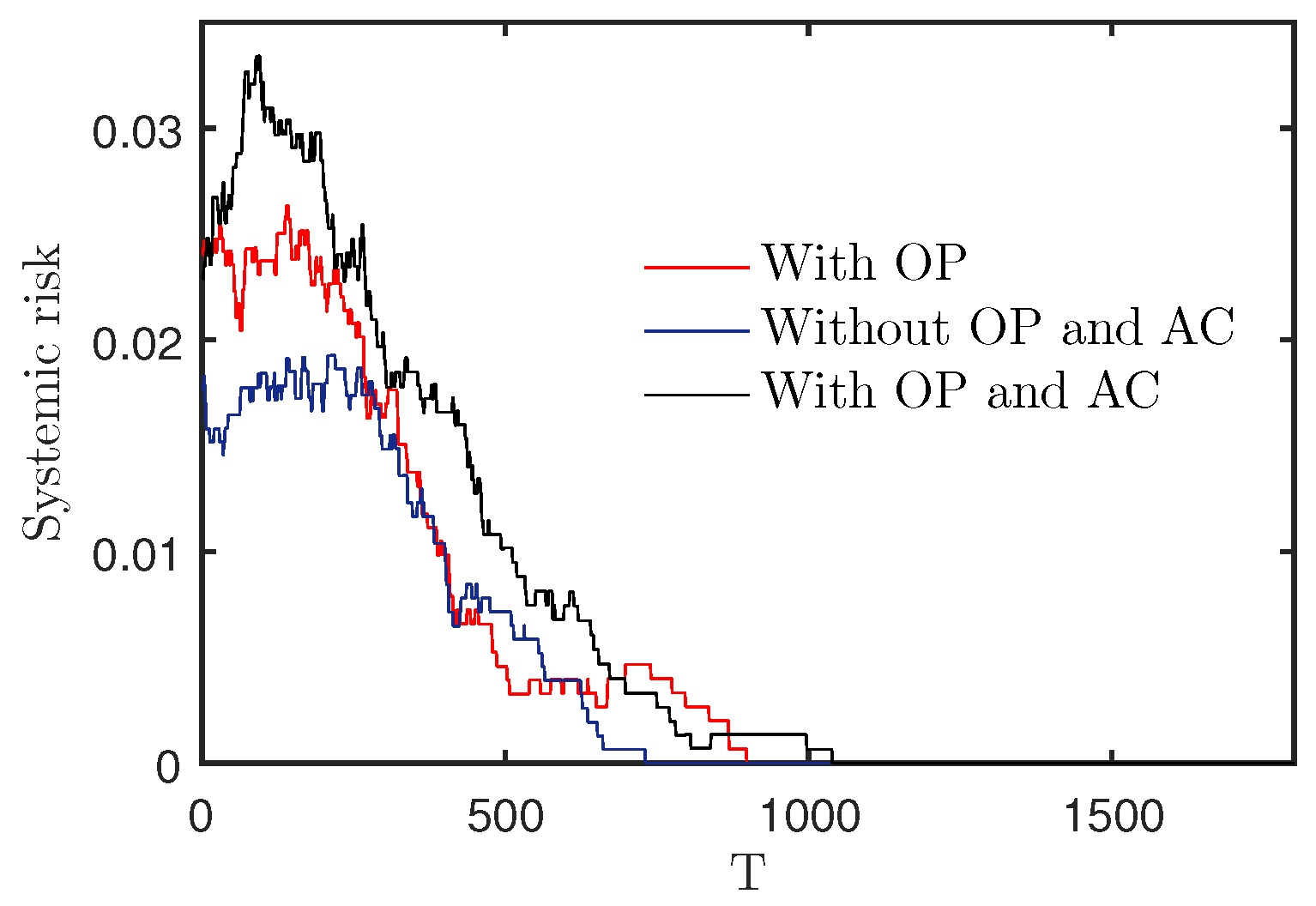
The effect of correlated assets and overlapping portfolios on systemic risk is seen in Figure 6. Due to banks’ simultaneous inclusion of the same assets, there is an indirect link between the banks’ respective portfolios. The difference of the price of an asset affects not only many holding institutions, but also the prices of other assets related to the asset. The change of assets of one bank will influence other banks through the overlap of assets portfolio and the correlation of assets. As demonstrated in Figure 6, the banking network system’s risk is increased by the overlapping portfolios and asset correlation. These two indirect transmission channels are crucial for the financial network system’s risk assessments.

This effort will investigate the suggested model from the following angles in order to confirm its efficacy in describing the risk contagion: (I)The contribution of investment-related factors to the spread of risk; (II) Influence of deposit interest rate and deposit variation on banking system stability; (III) A bank’s reserve ratio’s impact on the stability and liquidity of the banking network system; (IV) Influence of assets correlation coefficient on banking network system stability; (V) Evolution process of the systemic risk with different interbank lending network structure and interbank lending rate.

3.1. Analysis of Factors Related to Investment

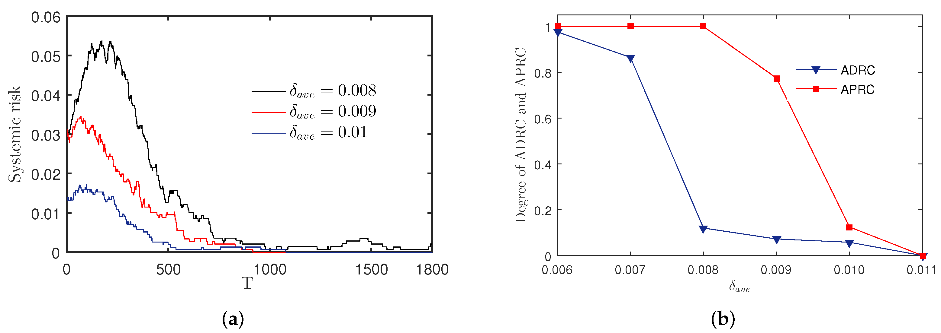
In the real financial system, the average ROI serves as a proxy for the overall state of the market [55]. The systemic risk of banks with various average ROIs is displayed in Figure 7a. The average level of risk contagion and the average likelihood of risk contagion under various average ROIs are depicted in Figure 7b. The financial network system is shown in Figure 7a to be more stable the higher the average ROI. The banking network system stabilizes at about 1000 steps when the average ROI is between 0.001 and 0.009. When the average ROI is 0.08, the financial network system is always dangerous.This is due to the fact that the average ROI is too low and there is not a sufficient interest differential between the interest on deposits and the return on investments, which causes the bank’s profitability and risk-taking capacity to diminish. As a result, the banking network always carries the systemic risk when the rate of return on investment is too low. This is due to the fact that the average ROI is too low to produce a sufficient margin between bank expenses and investment revenue, which causes banks’ profitability to drop and weakens their ability to resist risk. The probability of risk contagion in the financial network system is 100%, as shown by Figure 7b. noting that when the average ROI is 0.008, the average degree of the infection drastically decreases in comparison to when the average ROI is 0.007.The likelihood of risk contagion will be significantly lower when the average ROI approaches 0.01 than when it is 0.009. The results given above demonstrate that the stability of the financial network system is significantly impacted by the average ROI. The stability of the banking network system is improved by raising the average ROI. There will not be any risk contagion when the average ROI is 0.011, but there may be isolated bank failures in the banking network system.

The choice of a bank’s investment strategy is just as crucial to the system’s stability as the average ROI. In the financial market, the return on investment of various investment goods varies generally, and the ROI of the same investment product varies over time. A prudent portfolio choice is crucial to a bank’s ability to manage risk. Figure 8a depicts the systemic risk for various ROI variances. Figure 8a demonstrates that the systemic risk of the financial network system increases with increasing $\theta$ value. Furthermore, while the financial network system can become stable when $\theta$ is between 0.02 and 0.04 and when $\theta$ is between 0.06 and 0.08, systemic risk will always exist in the banking network system.The likelihood of significant bank losses will increase because to the high ROI fluctuation, which will also result in a liquidity crunch. When $\theta$ is large, the systemic risk rises sharply; banks with low net assets and low liquidity may experience excessive investment losses; the total investment income is insufficient to cover the borrowing costs and deposit interest, which will result in bankruptcies; and finally, $\theta$ is large, the systemic risk is increased. The likelihood of substantial loss is low when $\theta$ is small. By borrowing money and receiving other investment returns, banks can make up for the loss. Due to the extensive storage of high-risk investment goods during the 2008 financial crisis, which led to enormous investment losses, several financial institutions went out of business. The average level of risk contagion and the average likelihood of risk contagion for various values of $\theta$ are depicted in Figure 8b. Figure 8b shows that when $theta$ is less than 0.03, both the likelihood of risk contagion and the degree of contagion are low. When $\theta$ is 0.04, there is a 77.5% chance of risk contagion, although the level of contagion is low. The chance of risk contagion in the network is 100% when $\theta$ is bigger than 0.05, but the level of contagion remains relatively constant. The level of contagion dramatically rises when $\theta$ is between 0.05 and 0.07. The aforementioned findings demonstrate the critical role that sound investment strategies play in maintaining the financial network system’s stability.

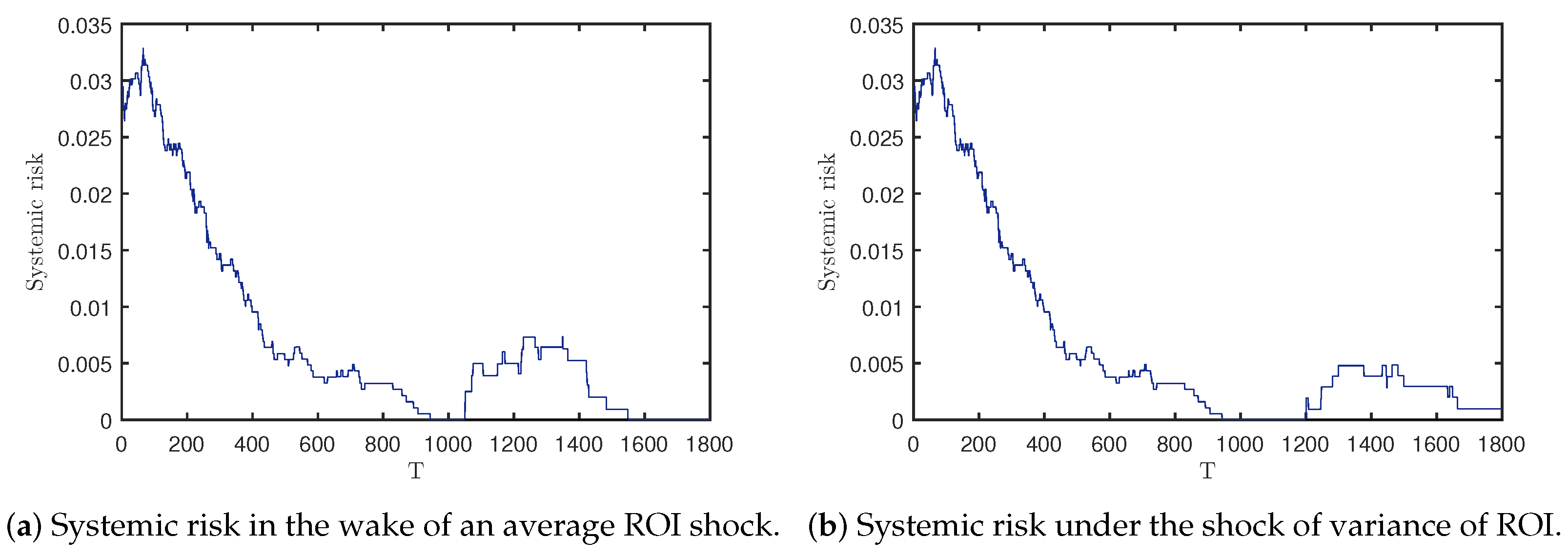
In order to wash away the variability due to the arbitrariness of the initial conditions, We investigate how various characteristics affect the development of a stable banking system under various shocks. Figure 9 displays the banking network system’s evolution results in response to the shock of investment. As shown in from Figure 9a, when the average ROI changes suddenly (from 951 steps to 1200 steps), the banking system will generate systemic risk. However, bank failures did not occur until 300 steps later (i.e., step 1050 showed systemic risk). This result indicates that the banking system can withstand some risks when the average return of investment changes suddenly. However, when the average rate of return is always low, the liquidity within the banking system will become increasingly inadequate, until leading to the bankruptcy of some banks. Systemic risk under the shock of variance of ROI is depicted in Figure 9b. Figure 9b demonstrates that the increase in variance of ROI leads to risks in the banking system, but it takes a long time for systemic risks to emerge. However, the average rate of return of the banking system remains unchanged. Therefore, banks with insufficient liquidity can obtain temporary liquidity through interbank lending, thus delaying the occurrence of systemic danger.

3.2. Analysis of Factors Related to Deposit

Banks’ primary revenue comes from deposits, and their primary expense is interest on deposits. The main source of banks’ profits is the interest margin between investments and deposits, hence the deposit rate has an impact on the profitability of banks. Figure 10 depicts how the financial network system has changed as deposit rates $r_a$ have varied. The deposit rate has a greater influence on the stability of the financial network system, as shown in Figure 10a. Risk to the financial network system that is systemic grows with the deposit rate. The network system for banks can become stable when the deposit rate $r_a$ is between 0.003 and 0.004. However, the systemic risk has always existed in the network system for banks, and it rapidly increases when $r_a$ reaches 0.005. Figure 10b demonstrates that there will not be any risk contagion in the financial system when $r_a$ is smaller than 0.003. Both the probability of contagion risk and its severity increase fast when $r_a$ is higher than 0.003. The financial network system exhibits the phenomenon of high probability of contagion and low degree of contagion risk when $r_a$ is between 0.004 and 0.005. When $r_a$ reaches 0.006, the banking system will collapse completely.

This finding demonstrates that the stability of the financial network system is perceptive of the rate of deposit and that the deposit rate might fluctuate significantly, even little. This is due to the fact that deposits now account for a sizable amount of the system’s funds and are the primary source of banks’ liquidity in the existing banking network structure. A minor increase in the deposit rate will cause a substantial decline in bank profits, which will eventually cause some banks in trouble to go bankrupt.

The overall number of deposits will change depending on the macroeconomic situation and deposit rate. Figure 11 depicts the evolution of the financial network system under various deposit volatility conditions. As observed in Figure 11a, the banking network system’s risk drops marginally with an increase in deposit volatility when it is less than 0.15, which is an intriguing result. This outcome demonstrates that deposit A modest amount of variation can increase the financial network system’s stability. Figure 11b demonstrates that the banking network system exhibits a phenomena of high probability of infection and low degree of contagion when the deposit volatility is smaller than 0.15. Banks that have restricted ownership rights and poor liquidity are more likely to collapse when deposit volatility is high because of a lack of liquidity when deposits contract.

Risks to the financial system will result from the shock of deposits. The outcomes of the banking network system’s evolution under the shock of deposits are shown in Figure 12. Figure 12a illustrates how a change in the deposit rate can immediately result in an increase in the interest that banks pay, this is going to affect the financial system’s liquidity. According to the outcome, the banking sector is more susceptible to variations in deposit rates. The financial system’s stability is not significantly impacted by deposit volatility, as seen in Figure 12b. When the variance is 0.3, only a small number of bank failures will occur. Although the variance of bank deposit is large, the total savings of banks have not changed much. Therefore, the liquidity of the banking system can still maintain a good level. The interbank market allows banks with insufficient liquidity to borrow money. As a result, there is little effect of deposit volatility on the financial system.

The deposit in this paper obeys normal distribution. If other parameters remain unchanged (the corresponding parameters in Figure 5), and the average value of deposits is large enough and the fluctuation of deposits of banks is small enough, then the banking system will be stable (the initial state of banks in this paper is random), and there will be no systemic risk after a period. This is because, if a stable banking system does not have external shocks, and the average ROI is sufficient, and the volatility of ROI is not large, then the banking system will operate stably, and the impact of some small fluctuations will be absorbed by the banking system itself, and the banking system can resist some small fluctuations. The change in deposit, the change in deposit interest rate, and the change in return are some of the constant causes of systematic risk. Therefore, even if the evolution time is long enough, the system will not have systemic risk if the system parameters do not change (for instance, after 1000 steps in Figure 5).

For a stable banking system, if the deposit related parameters change, then the banking system may produce risks. In Figure 13, when the average deposit amount changes to 700 at 951 step and lasts for 250 steps, the banking system will change from risk-free to risky. Furthermore, systemic risk will last for a long time, and eventually become risk-free. In this model, with other parameters unchanged, if the average deposit amount is changed to 700, it will take few steps on average to generate systemic risk. In addition, if the volatility of bank deposits is too large, it is also prone to systemic risk. Through a lot of simulation, if the volatility of deposits exceeds 0.28, then there will be systematic risk in the network until all banks fail, but this will take a long time (more than 30,000 steps when the volatility is 0.28).

The usage of bank money may be constrained by the deposit reserve ratio, which has a substantial effect on the financial system’s stability. Figure 14 depicts how the financial network system has changed as a result of various bank reserve ratios. Figure 14a demonstrates that the financial network system’s systemic risk decreases when the ratio of deposit reserves falls. This is due to the fact that as the percentage of deposit reserves rises, the sum of money available for investment decreases, decreasing the return on investment. As a result, the margin between investment and deposit decreases, increasing the possibility of default and decreasing the ability of banks with low net assets to handle risks. As illustrated in Figure 14b, There is relatively little chance of risk contagion in the financial network system when the deposit reserve ratio is less than 0.2. The likelihood of risk contagion increases significantly as the deposit reserve ratio goes from 0.2 to 0.25, while the level of contagion stays relatively constant. The shift in the contagion degree increased gradually as the deposit reserve ratio rose from 0.2 to 0.4.

3.3. Analysis of Factors Related to Interbank Lending

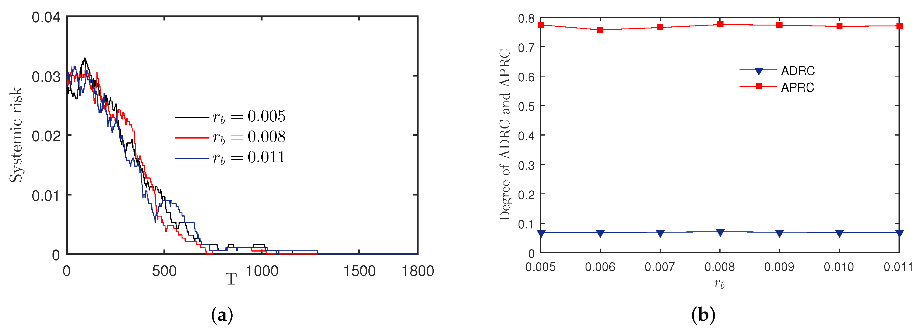
The effect of the interbank offered rate on the stability of the banking network system is depicted in Figure 15 Changes in the interbank offered rate have little effect on the stability of the financial network system, as shown in Figure 15a. This verdict is really intriguing. Because of the temporary lack of liquidity in the real financial network, the interbank offered rate has a tendency to rise dramatically. For instance, the overnight interbank offered rate (HIBOR) in Hong Kong increased to 66.82% in 2016 as a result of a lack of liquidity. However, in reality, the systemic risk is not brought on by the high interbank offered rate. Figure 15b demonstrates that under various interbank offered rates, the likelihood and the extent of the financial network system’s risk contagion alter relatively little. Lending between banks is a type of short-term borrowing. The small fraction of short-term interest costs that make up banks’ net assets can be easily absorbed by their earnings. The banking network system’s interbank linkages between banks limit banks’ borrowing activities. Figure 16a demonstrates that the more connections there are between banks when the likelihood of interbank connection is 0.01, 0.02, and 0.05, the more stable the system is. However, there is minimal change in systemic risk between $p_{ij}=0.05$ and $p_{ij}=0.06$. Low connection makes it challenging for banks to borrow in the interbank market, which will result in a lack of liquidity for banks to borrow and a default. Figure 16b demonstrates that the probability of risk contagion and the degree of risk contagion in the financial network system remain unchanged when the probability of connection surpasses 0.03. The likelihood of borrowing money does not change as connectivity grows; nevertheless, when the banking network system runs out of cash and borrowing becomes challenging, banks with low net assets and insufficient liquidity are more likely to default.

3.4. Analysis of Factors Related to Assets Correlation

Figure 17 shows the impact of different correlations between assets on risk contagion. In Figure 17a, the greater the positive correlation between assets prices, the greater the systemic risk in the banking network system. The positive correlation between assets aggravates the risk contagion. When the price of one asset falls, the price of other assets related to it will also fall to varying degrees, making the crisis more destructive in the banking network system and covering a wider range. The negative correlation between assets prices means that when the price of one assets falls, the price of other related assets rises instead, which weakens the impact of the depreciation of individual assets on the system. The simulation results are consistent with Markowitz’s portfolio theory [56]. According to the principle of decentralized investment, the smaller the correlation between investment assets, the smaller the risk. Therefore, the risk can be dispersed by choosing a portfolio of financial products with negative correlation. Figure 17b demonstrates how the assets’ negative correlation lowers systemic risk. The chance of the network spreading contagion is significant when the assets correlation coefficients are 0, 0, 02, and 0, 03, but the average level of contagion is low. When an asset’s correlation coefficient is higher than 0.04 there is a high danger of contagion and a high level of contagion in the banking network system. The probability distribution of the number of surviving banks exhibits two distribution centers when the positive correlation between assets is high, as seen in Figure 18. In Figure 18, the final 180 banks in the banking network system are distributed when the correlation coefficient between assets is 0.03. When the correlation coefficient between assets is 0.04, there are either very few or close to 180 last-standing banks in the banking system. When the correlation coefficient between assets is 0.05, there is a larger likelihood that only a small number of banks will survive, meaning the banking network system is more likely to fail, however it is also possible that the majority of banks will.

3.5. Market Density and Average Asset Density

When the diversity of the average assets is large, the more types of investment products each bank has on average. Figure 19 Results of the financial network system’s evolution at various levels of average asset diversity. as shown in Figure 19a, the more average assets banks own, the Bank Financial Network System has fewer systemic hazards. Figure 19b shows that when the average assets diversity is 2 and 4, the Bank Financial Network System has a high level of risk contagion and a high possibility of it, and the banking network system is easy to collapse. The likelihood of risk contagion in the banking network system is higher when the average assets diversity is greater than 8, yet the risk contagion is relatively low. Furthermore, when the average asset variety increases, the likelihood of risk contagion reduces. In the banking network system, when the average diversity of assets held by banks is small, once external shocks have an impact on the design, the loss of assets may have a greater impact on the system, and if there are not enough assets to share risks, the risk contagion is more likely to occur. With the increasing diversity of assets, the ability to share risks among different assets is gradually strengthened, the impact of changes in asset prices on banks is reduced, and the probability of contagion is also gradually reduced. The probability allocation of the number in remaining banks is displayed in Figure 20. The number of banks that finally survive in the banking network system is very low when the diversity of the average assets is 4, and the banking network system is in a condition of collapse. When the average assets diversity reaches 6, there are two distribution centers in the number of enduring banks, that is, the banking network system collapses, or the banking network system ultimately has a higher number of surviving banks, which the banking network system is susceptible to risk contagion. The number of surviving banks in the financial network system always remains at a high level when the diversity of the average asset is between 8 and 10.

The size of market density impacts the number of assets banks hold when the likelihood of the relationship between banks and assets is fixed. Figure 21 depicts how the financial network system has changed as market densities have changed. Figure 21a demonstrates that when market density increases, systemic risk also rises. The greater the market density, the greater the possibility that each asset will be held by multiple banks, raising the chance of risk contagion. The smaller the market density is, the less probability each asset will be held by multiple banks, decreasing the network’s indirect risk contagion channel. As shown in picture Figure 21b, when the market density is less than 1.4, the likelihood of the system being contagious rises progressively, while the average degree of the contagion increases slowly. When the market density increases from 1.4 to 2, the average contagion degree increases significantly, but the system’s risk contagion probability eventually lowers. The banking network system is characterized by “robustness and fragility”. That is, the findings of Caccioli’s [39] research are consistent with the likelihood of threat contagion in the network system being lowered, but once it happens, the banking grid system will collapse. When the market density reaches 2, each asset is more likely to be held by multiple banks. On the one hand, the channels of risk indirect transmission increase, and the banking network system is more prone to crisis contagion. On the other hand, when the market density is very high, the numeral of banks holding the increases of the same asset, and the average proportion of banks holding the assets decreases, which reduces the possibility of a substantial price decline of the assets, thus maintaining the stability of asset prices. The above two factors are a game relationship and show a “winner-take-all” phenomenon. The probability allocation of the remaining banks is shown in Figure 22. As can be seen from Figure 22, when the market density is 0.8, the number of enduring banks is very high. When the market density is 1.7, the number of average surviving banks is lower than that in the market density of 0.8, and the variance is larger than that in the market density of 0.8. When the market density is 2, there are two distribution centers in the number of surviving banks, that is, either the banking network system collapses, or the banking network system ultimately has a higher number of surviving banks.

4. Conclusions

A banking network system is a complicated network system made up of numerous banks and their connections. In addition to being directly connected to the interbank loan market, the overall risk is indirect ties to the shared asset investments between banks. Existing research either focuses on the interbank market or the overlapping portfolio of bank investment, which can not accurately model the banking network system. The portfolio overlapping and asset correlation are essential reasons for indirect risk contagion. Current studies seldom consider the correlation between different assets. It causes the financial network system’s current risk models to either underestimate or incorrectly determine the likelihood and severity of the risk contagion brought on by the indirect contagion. Additionally, several of the assumptions used in recent studies are not realistic. For instance, the return on investment is fixed, and the depreciation of sold assets cannot be used to increase liquidity. The earlier models cannot accurately reflect the current state of the banking grid technique because of the inaccuracy of the study hypothesis. This study develops a multi-channel threat contagion network model that considers portfolio overlap, interbank lending, and asset correlation. This model allows banks to restock their liquidity by selling assets since “the rate of return on investment is stochastic.” According to this model, variations in asset prices are dispatched via the channels of portfolio overlaps and asset correlation, impacting the overall health of the banking network system. As a result of the quantitative and qualitative analysis of several variables affecting the stability of the banking system, the following findings with significant speculative value and managerial importance are drawn:

(I) The portfolio overlapping and support correlation are indirect transmission channels of credit risk, which improve the likelihood and degree of threat contagion.

(II) The financial grid system will be more stable with a higher average ROI. If the average ROI is excessively low, banks’ profits will typically be zero or negative, making banks less able to absorb risks and resulting in a constant systemic threat to the banking grid system. The systemic hazards to the financial network system are inversely correlated with ROI volatility. For the solidity of the banking network system, prudent investment practices are very crucial.

(III) The deposit rates have an influence on bank solidity. The systemic risk increases with the deposit rate. The systemic threat to the financial network system will rise if deposit volatility exceeds a specific threshold. The solidity of the monetary network system may be significantly increased by lowering deposit volatility and deposit interest rates.

(IV) Increased deposit reserve ratios decrease investment profit, which lowers banks’ ability to manage risks and raises systemic threats.

(V) The solidity of the banking network system is not significantly impacted by changes in interbank offered rates. The solidity of the banking network technique can, up to a point, be improved by an increase in interbank connections between banks.

(VI) The positive correlation between assets plays an aggravating role in the process of impact contagion, and the destructiveness of the crisis in the banking network system is more extensive. The negative correlation between assets prices can weaken the impact of the depreciation of individual assets on the banking network system.

(VII) The more kinds of assets banks own, the more risk-sharing ability among different assets is enhanced, and the systemic risk is smaller.

(VIII) The higher the market density, the more possibility each assets is held by multiple banks, which boosts the chance of risk contagion. However, at the same time, the number of banks holding the same assets increases, and the average proportion of banks holding the same assets decreases, which can maintain the stability of assets prices. When the market density is high, the game between these two factors leads to the whole banking network system showing the characteristics of “robust and fragile”.

This study focuses on how the banking system’s risk might spread through various channels and offers a framework for a quantitative examination of systemic risk in the context of macroeconomic changes. However, there are also study limitations in this paper: the article does not set the investment preferences of banks, but in the real banking system, different banks have different investment preferences. In addition, the inter-bank lending relationship of banks is relatively fixed, that is, a bank only lends to a small number of banks, and the network relationship between banks is stable. Although this work reflects the reality to a certain extent, it still lags behind the performance of the real banking system. Secondly, some of the assumptions in the paper are too strict, such as the limit of the investment proportion, the range of the volatility of the yield, etc. Future research can be enriched and developed on this framework, such as the study of the contagion risk considering the heterogeneity of banks and assets and the investment preference of banks. Future works can also study the impact of specific shocks and asset-specific correlations on risk contagion. The network structure of banks and investments in this work uses a stochastic network. We can examine the stability of the monetary network system under various network configurations in the future. The actual data can also be used for observed research.