Research on the Detection and Measurement of Roughness of Dam Concrete Layers Using 3D Laser Scanning Technology

Abstract

The roughness of the interlayer concrete, which is an important index for the construction of dams, affects the mechanical properties of the interface between new and old concrete. The traditional monitoring method cannot satisfy field measurements. Therefore, this paper proposes a concrete surface roughness measurement method based on 3D laser scanning technology and implements 3D point cloud calculations. Two layers of specimens with same concrete mix proportion were poured 28 days apart, and a splitting tensile strength test of the superimposed specimen was carried out. Four groups of experiments (MR-S, MR-N, MR-15, and MR-35) tested the interlaminar tensile splitting strength of nine 150 mm cubic specimens on the 3rd, 7th, 14th, and 28th days, respectively. Filling volume, mean amplitude, surface area expansion rate, normal angle std. dev., and curvature std. dev. were measured in the study. The results showed that as the surface roughness of the concrete increased, as did the flushing pressure. The splitting strength of the concrete interface after it solidified increased with age. At 28 days, the splitting strength of MR-15 was higher than that of MR-35. The mean amplitude and the normal angle std. dev. of the rough surface could replace the traditional filling volume index. The new 3D point cloud calculation method for calculating concrete surface roughness was proven by experiments to have good performance.

1. Introduction

Coastal water conservancy projects such as sea dikes and dams are barriers against natural disasters such as typhoons, floods, and tides. These projects are also an important guarantee for the development of the national economy and the well-being of people. Unfortunately, the negative impact of tidal dry and wet cycles and temperature changes on the durability of concrete, as well as strong winds, large waves, storm surges, and heavy rain caused by natural disasters such as typhoons, can damage seawalls and dams, which can have a significant impact on the safety and integrity of these structures and the people and communities they protect. Thus, it is essential to have a proper assessment of the condition of these structures to guarantee their safety and longevity. Since a concrete layer is a weak surface, the strength of the layer’s performance will affect the integrity, permeability, and corrosion resistance of the concrete structure, thereby endangering the safety of the structure, so timely reinforcement is required [1,2]. Among the existing reinforcement techniques, scouring is a method that uses a high-pressure water gun to wash the surface of concrete to expose fine sand, coarse aggregates, etc. [3]. It can increase the roughness of the interface between the upper and lower layers of the concrete and improve the bonding strength and shear resistance of the layer. Furthermore, concrete surface punching technology is widely used to improve the mechanical properties of the interface between new and old concrete.

The scouring effect of concrete is usually evaluated by its roughness [4,5,6,7]. In the detection of surface roughness, the basic principles can be divided into two categories: the point–line relationship calculation based on “line” sampling, or the volume–area relationship calculation based on “surface” sampling. Among the processing methods based on “line” sampling, the most representative are mechanical stylus, profile texture meter, and PDI (processing of digital images). The detection methods based on “surface” sampling mainly include concrete surface profiles, the sand patch test, water accumulation method, and slit-island method [8,9]. Generally, a method based on “surface” sampling has higher accuracy than one based on “line” sampling because more combined surface information is collected and used for calculation. In the case of repeated sampling, the fluctuation of the detection results is smaller [10]. In terms of non-digital measurement methods, a detection method based on “surface” sampling is a comprehensive evaluation comprising of quantitative analysis, damage to a rough surface, testing costs, portability of testing instruments, contact with rough surfaces (whether pre-treatment or post-treatment is needed), accuracy, and other factors [11]. As a representative option, the sand patch test stands out by virtue of its simple and clear principle, simple operation, and basic avoidance of damage to rough surfaces [12]. However, the method is limited by various constraints and is often less practical in engineering practice than in theory. As a result, the accuracy of sand patch test measurement data is insufficient and the collection efficiency is low. The sand patch test also cannot be digitized to inform the detection process and results. As this demonstrates, traditional measurement techniques cannot meet the needs of the times due to the continuous advancement of science and technology and the increasing demand for spatial three-dimensional (3D) information. Different from the point-to-line and line-to-surface single-point operation modes in traditional measurements, 3D laser scanning adopts the laser ranging method to record the massive and dense 3D coordinate value, reflectivity, and texture information on the surface of the measured object [13,14,15]. Based on the computer system and laser point cloud algorithm, the 3D model of the measured object and its line, surface, volume, and other data can be quickly obtained. Such 3D laser scanning has the advantages of high accuracy, high efficiency, quantification, and modeling, and realizes the leap from non-digital measurement to digital measurement of concrete surface roughness [16,17].

Surface-based 3D laser scanning measurements have been reported by many authors [13,18]. Tsakiri et al. used planes fitted to point clouds when estimating the deformation of a sea-lock [19]. In tunnel monitoring, Van Gosliga et al. modeled a tunnel with a cylinder [20]. Chang et al. developed a structure surface analysis program [21]. The surface data, such as the degree of surface deformation, can be easily obtained by using statistical regression and polynomial methods. Rosser et al. used 3D laser scanning to monitor changes to coastal cliff faces [22]. The results demonstrated that 3D laser scanning can be used to quantify cliff failures with previously unattainable precision. Monserrat et al. monitored land deformation using repeated 3D laser scanning and estimated the deformation parameters using local surface matching [23].

In addition, 3D laser scanning technology has been applied and achieved good results in the fields of surveying and mapping engineering, deformation monitoring [24,25,26,27], mine surveying, cultural relic protection, archaeological exploration, agricultural data collection, etc. [28,29,30,31,32]. As 3D laser scanning had good application prospects, this study adopted the following hypotheses:

• When the flushing pressure increases, the surface roughness of the concrete will also increase;
• The splitting strength of concrete increases with its roughness;
• The mean amplitude (mm), surface area expansion rate, normal angle standard deviations (std. dev.), and curvature std. dev. can replace the traditional filling volume as the roughness index of concrete.

The study used 3D laser scanning technology to efficiently and accurately reconstruct a concrete surface in order to study the roughness of concrete and the proposed algorithms and indicators.

2. Materials and Methods

2.1. Concrete Material and Mix Proportion

Baihetan concrete was used in this study. The concrete mix proportions are shown in

Table 1. Mix proportion of concrete (kg/m³).

Water	Cement	Fly Ash	Sand	Small Boulders	Water Reducing Agent	Air Entraining Agent
122	197	106	691	1284	2.121	0.121

.

Table 2. Main chemical composition of concrete (%).

SiO2	Al2O3	CaO	Fe2O3	K2O	MgO	Na2O	TiO2
19.591	4.430	64.033	2.843	0.630	1.323	0.106	0.266

shows the main chemical composition of concrete.

The coarse aggregate used had an apparent density of 2810 kg/m³, a bulk density of 1515 kg/m³, mud content of 0.3%, soil content of 0%, an index of crushing value of 5%, needle flaky content of 4.5%, and ruggedness of 2%.

2.2. Specimen Design

The specimen in this study was 150 mm × 150 mm × 300 mm in size and was cast in two equal layers, namely layers A and B. Layer A and layer B were both 150 mm × 150 mm × 150 mm in size.

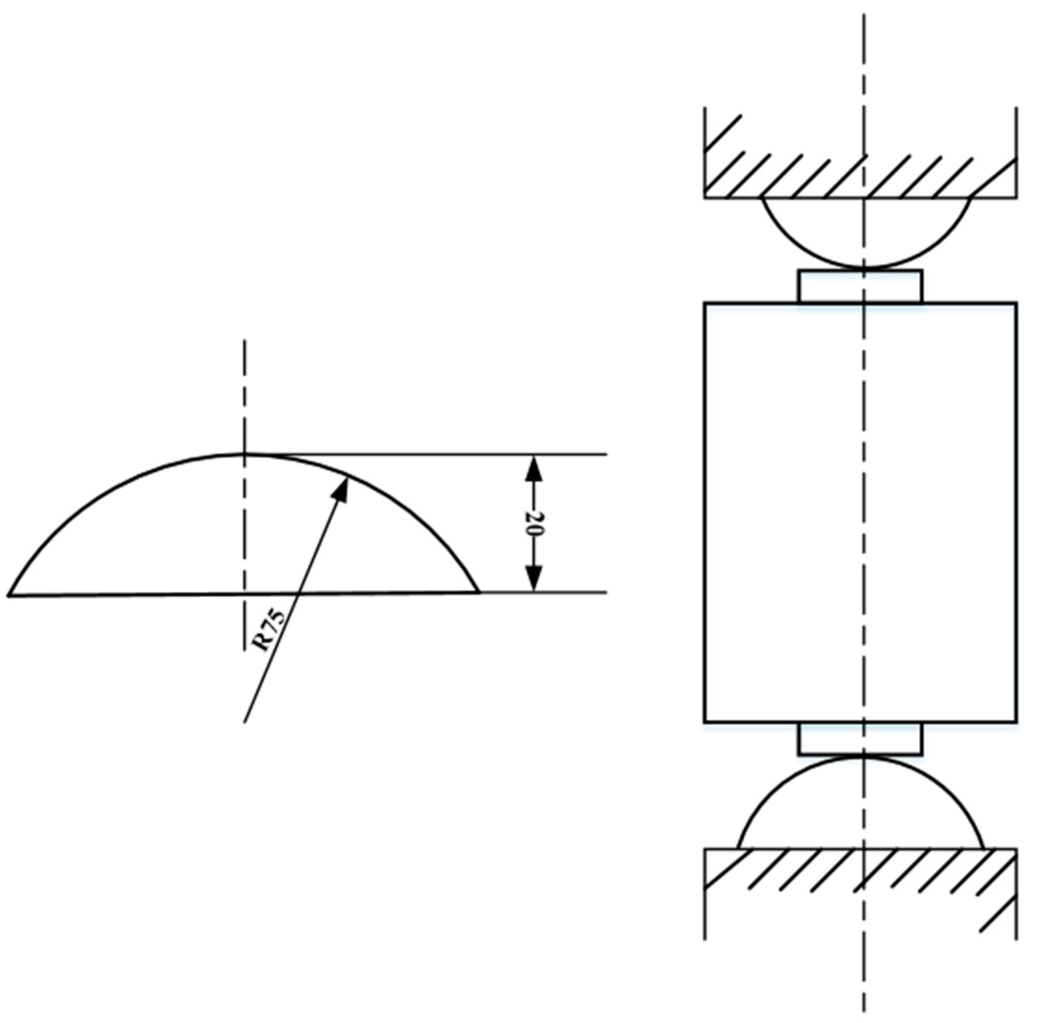
In this experiment, the roughness of the interface of the test piece was set by the scouring method. Pressures of 15 MPa and 35 MPa were selected to carry out the scouring treatment on the specimen, and two sets of controls, without scouring (N) and with integral pouring (S), were adopted. We used a press to carry out the split tensile strength test. As shown in Figure 1, there was an iron cushion strip on the top and bottom of the press to simulate the splitting process. Nine 150 mm cubic specimens were tested at 3, 7, 14, and 28 days for the interlayer tensile splitting strength of concrete according to the Chinese standard DL/T 5150–2017. The mean values were recorded.

2.3. Specimen Production

The specimens were cast in a cubic size of 150 mm × 150 mm × 150 mm. In the process of casting the specimens, layer A was first poured, and then we used a high-pressure water gun to finish them after a 3-day standard curing period. After 3 days of standard curing, the poured concrete A-layer specimens were tested in groups. The experiment was divided into three groups, one of which was set up as the control group without any treatment. The difference between the other two groups lay in the scouring strength of the specimen. The second group had a scouring strength of 15 MPa, and a third group had a scouring strength of 35 MPa.

Because there is usually a long pouring interval in actual projects, concrete layer B was added to layer A after a period of time. We chose to leave layer A for 28 days after the scouring treatment, and we poured concrete layer B according to the mixture ratio in Table 1. Before pouring layer B, the surface of the freshly poured concrete layer A specimen was soaked in clean water to ensure that the concrete specimens poured at different times had good contact. Following the completion of the first pour, the second pour smoothed the end face. Using the same method, a batch of rectangular parallelepiped specimens with a size of 150 mm × 150 mm × 300 mm was produced. The finished specimens were divided into 4 groups with ages of 3 days, 7 days, 14 days, and 28 days, and the mechanical strength test was carried out.

2.4. The 3D Laser Scanning and 3D Point Cloud Data Processing Algorithm

2.4.1. 3D Laser Scanning

In this study, a Roland LPX 3D laser scanner was used for the 3D scanning test to measure the surface roughness of concrete specimens. The scanner used a non-contact laser sensor to acquire information on the rough surface morphology, with a scanning speed of 37 mm/s and a scanning accuracy of 0.02 mm. We placed the object to be measured in the center of the table of the Roland LPX 3D laser scanner, with the rough surface vertical. In this way, accurate scanning results could be obtained, which could be used to analyze the actual situation of the object to be measured. The 3D scanning renderings are shown in Figure 2.

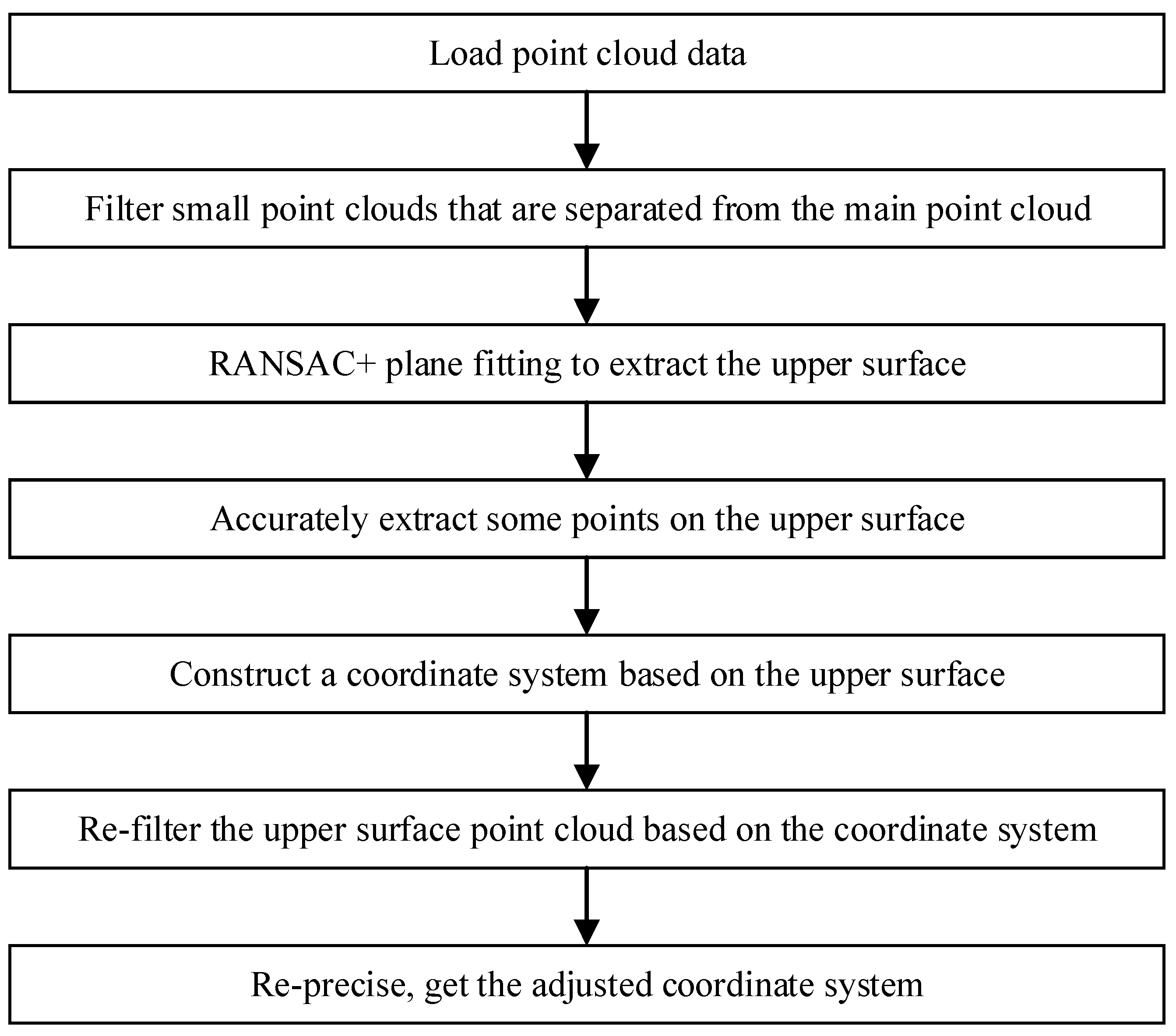
A flow chart of the 3D point cloud processing algorithm can be seen in Figure 3.

2.4.2. Point Cloud Filtering

Firstly, point cloud data were obtained from the 3D scanning. Small point clouds that separated from the main point cloud were filtered out. Then, the RANSAC+ plane fitting method was used to extract the upper surface, and some points on the upper surface were accurately extracted. Finally, a coordinate system based on the upper surface was constructed (Figure 4).

Random Sample Consensus, abbreviated as RANSAC, is an efficient and robust estimation algorithm. RANSAC obtained model parameters by selecting a small amount of sample data that met the conditions. Then, a consistent dataset was used to expand that dataset. Finally, the best-fitting model was obtained. The process was as follows.

From the point cloud data, three non-collinear points were selected, and their corresponding plane equations were calculated:

$$ax+by+cz+d=0$$

(1)

The distance $d_i$ from each point in the point cloud data to the plane was calculated as follows:

$$d_i=\frac{\left|a{x}_i+b{y}_i+c{z}_i+d\right|}{\sqrt{a^2+b^2+c^2}}$$

(2)

Calculate the std. dev. $\sigma$ of $d_i$; then, $\sigma$ can be used as a reference for selecting the value of t.

$$\sigma =\sqrt{\frac{{{\displaystyle \sum }}_{i=1}^n{\left(d_i-\overline{d}\right)}^2}{n}}$$

(3)

Among them, $\overline{d}=\frac{1}{n}{\displaystyle \sum }_{i=1}^n{d}_i$.

A threshold t was chosen. If $d_i$ < t, it was counted as an interior point. And $n$ was the number of interior points that could be calculated. After multiple iterative calculations, the plane with the largest number of interior points $n$ was selected, and the fitting plane was finally obtained. The upper surface was extracted using the RANSAC+ plane fitting method at the time.

2.4.3. Coordinate System Construction

RANSAC+ plane fitting was used to obtain the plane normal vector n and all the points on the plane from the point cloud (Figure 5a orange points).

$x_m$ was the average of all points on the plane, which represented the center point of the rectangle formed by each point on the plane. Then, as the vertex of the rectangle, $x_f$ was the farthest point on the plane from the center point $x_m$.

If constructing a rectangular auxiliary coordinate system with the midpoint of the rectangle as the origin, the plane normal vector $n$ was the positive direction of the z-axis, and $x_f-x_m$ was the positive direction of the x-axis. The transformation matrix from the auxiliary coordinate system to the initial coordinate system was:

$${}_A{}^{I}T=\left[\begin{array}{cccc}\frac{x_f-x_m}{\Vert x_f-x_m\Vert }& I_y& \frac{n}{\Vert n\Vert }& x_m\\ 0& 0& 0& 1\end{array}\right]$$

(4)

Among them,$I_y=\frac{n}{\Vert n\Vert }\times \frac{x_f-x_m}{\Vert x_f-x_m\Vert }$.

The rectangular coordinate system was set as the auxiliary coordinate system rotated 45 degrees around the z-axis, so the transformation matrix from the rectangular coordinate system to the auxiliary coordinate system was:

$${}_M{}^{A}T=\left[\begin{array}{cccc}cos\left(\pi /4\right)& -sin\left(\pi /4\right)& 0& 0\\ sin\left(\pi /4\right)& cos\left(\pi /4\right)& 0& 0\\ 0& 0& 1& 0\\ 0& 0& 0& 1\end{array}\right]$$

(5)

The transformation matrix from the initial coordinate system point to the rectangular coordinate system was:

$${}_I{}^{M}T={}_A{}^{M}T{}_I{}^{A}T$$

(6)

The result is shown in Figure 5b. The upper surface point cloud was re-filtered based on the coordinate system, and the result is shown in Figure 5c. The coordinate system was refined again, and the result shown in Figure 5d was obtained.

2.5. Research on 3D Laser Scanning Roughness

(a)

Filling volume was extracted from the obtained point cloud and calculated:

The point cloud density was uniformly sampled (down-sampling) (see the PCL library for the voxel grid) by a voxel grid where the leaf was 0.25 m. The absolute value of the z-axis direction of all points in the point cloud was found and used to calculate the filling volume:

$$v=\frac{S}{N}{\displaystyle \sum }_{i=1}^N\left|z_i\right|$$

(7)

where $z_i$ was the component in the z-axis direction of the $i$-th point in the point cloud, $N$ was the number of points in the point cloud, and $S$ was the area of the rectangle (if the rectangle became 150 mm in length, then $S$ = 150 × 150).

(b)

Calculation of mean amplitude:

$$l=\sqrt{\frac{1}{N}{\displaystyle \sum }_{i=1}^N{\left(n_{z,i}-{\overline{n}}_z\right)}^2}$$

(8)

${\overline{n}}_z$ was the average value of the unit normal vector of all point clouds in the z-axis direction.

(c)

Calculation and statistics of the normal vector:

The point cloud normal vector was the most important geometric feature of the 3D point cloud data. It represented the inherent characteristics of the data point in the entire collection and was one of the important bases for point cloud data processing. For the sampling point P, the local plane L was fitted according to its neighboring k points. This plane L could be expressed as:

$$L\left(n,d\right)=arg min{\displaystyle \sum }_{t=1}^k{\left(n·p_i-d\right)}^2$$

(9)

where $n$ was the normal vector of plane L, $\overline{p}$ was the centroid of the k neighboring points in plane L, and $d$ was the distance from point p to plane L. Through the eigenvalue decomposition of covariance matrix M, the eigenvector corresponding to the smallest eigenvalue of M was the normal vector of point p.

$$M=\frac{1}{k}{\displaystyle \sum }_{i=1}^k\left(p_i-\overline{p}\right){\left(p_i-\overline{p}\right)}^T$$

(10)

The estimated normal vector had no direction, and the normal vector needed to be redirected. The p coordinate of the sampling point was (x, y, z), and the angle between the normal vector of the sampling point and the z-axis direction of the rectangular coordinate system was:

$$\alpha =arc\cos \left(\frac{n·{\left[-x-y-z\right]}^T}{\sqrt{x^2+y^2+z^2}}\right)$$

(11)

It was stipulated that if $\alpha \le 90°$, then n would not change; if $\alpha \ge 90°$, then we let $n=-n$ to realize the fast global orientation of the normal vector.

We calculated statistics for the angles between the normal vectors and the z-axis direction of the rectangular coordinate system and calculated their proportions in each interval. The std. dev. of the angle between the normal vector and the z-axis of the rectangular coordinate system was:

$$\tau =\sqrt{\frac{{{\displaystyle \sum }}_{i=1}^m{\left({\alpha }_i-\overline{\alpha }\right)}^2}{m}}$$

(12)

where $m$ was the total number of normal vectors, $\overline{\alpha }=\frac{1}{m}{\displaystyle \sum }_{i=1}^m{\alpha }_i$.

(d)

Surface area expansion rate calculation:

The unit normal vector of each point in the point cloud (N = 8) needed to be calculated. Then, the expansion area calculation formula was:

$$s=\frac{S}{N}{\displaystyle \sum }_{i=1}^N\frac{1}{\left|n_{z,i}\right|}$$

(13)

where $n_{z,i}$ was the z-axis component of the unit normal vector.

(e)

Curvature statistics:

Curvature was an important indicator reflecting the surface characteristics of the target object, which reflected uneven change in the target object. $p_i$. was set as a point in the point cloud data. After adjusting the direction of the normal vector, the curvature $c{\mu }_i$. of point $p_i$. was calculated as:

$$c{\mu }_i=\frac{{\lambda }_0}{{\lambda }_0+{\lambda }_1+{\lambda }_2}$$

(14)

The curvature of all point cloud data and their distribution ratio in each interval needed to be obtained. The calculation formula for the average curvature $\overline{c\mu }$ was:

$$\overline{c\mu }={\displaystyle \sum }_{i=1}^N\left|c{\mu }_i\right|$$

(15)

where N was the total number of point clouds and $\mathrm{c}\mathsf{\mu }$ was the curvature of each point.

The std. dev. of the curvature was:

$$\phi =\sqrt{\frac{{{\displaystyle \sum }}_{i=1}^N{\left(c{\mu }_i-\overline{c\mu }\right)}^2}{N}}$$

(16)

3. Results

3.1. Research on Roughness of 3D Laser Scanning

The roughness indices selected for this study were filling volume (mm³), mean amplitude (mm), surface area expansion rate, normal angle standard deviation, and curvature standard deviation. The average values for these indices, as measured by 3D laser scanning, are presented in

Table 3. Concrete surface roughness index.

	V/mm3	L/mm	s	τ	φ
MR-N	29,897.850	0.513	1.146	0.266	0.000
MR-15	57,754.982	0.878	1.093	0.364	6.747
MR-35	163,286.117	2.554	1.469	0.513	0.001

for each group of specimens, along with their respective standard deviation (std. dev.). It is worth noting that the standard deviation shown reflects the degree of variation among individual results within a group.

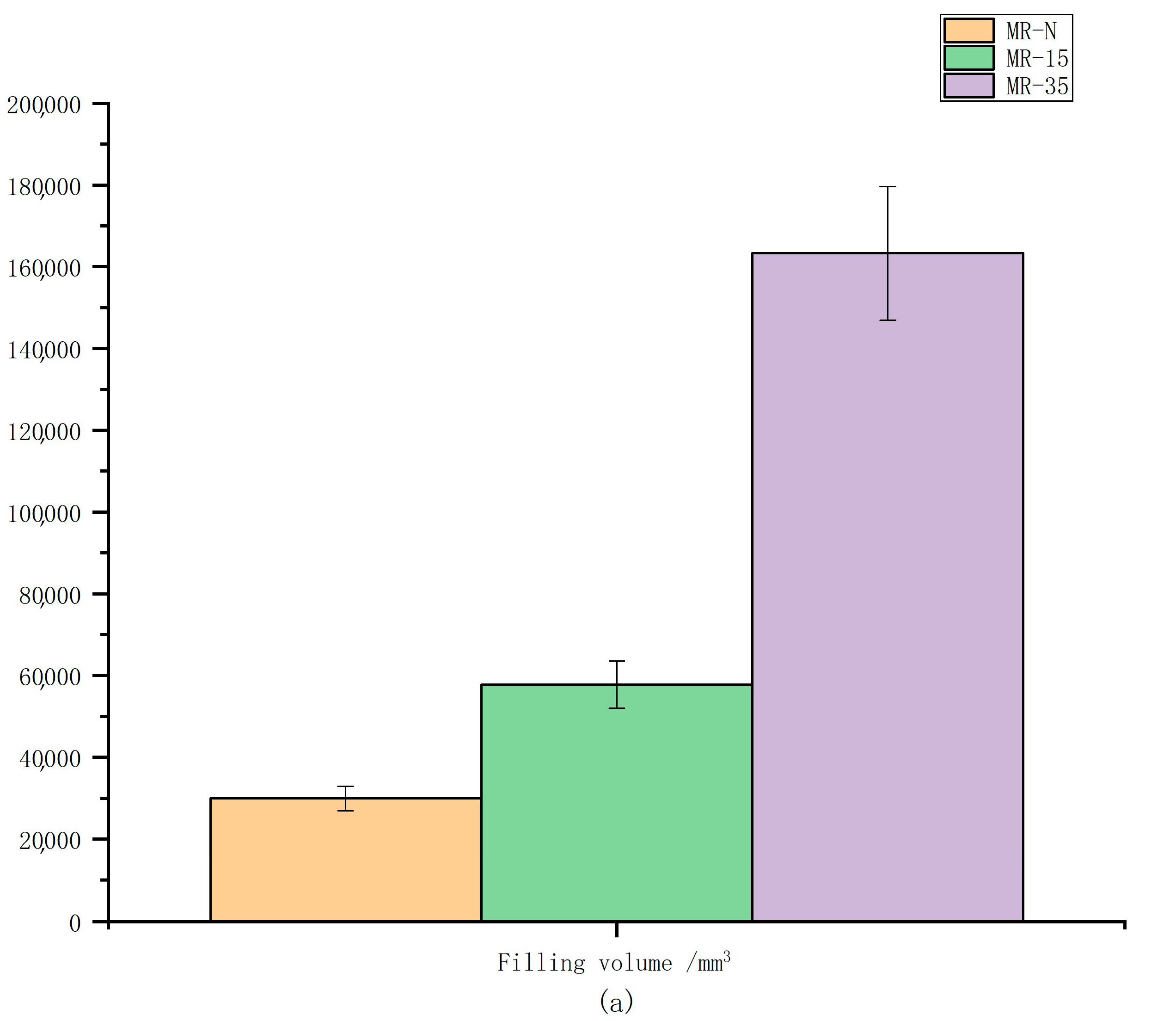
Figure 6 showed the change trend of each index under various working conditions. The x-axis represents the working condition, and the y-axis the numerical value of indicators. Overall, the indicators of the 35 MPa flushing treatment group were significantly higher than those of the other two groups. Except for the two indices of surface area expansion rate and curvature std. dev., the values of other indexes in the 15 MPa treatment group were higher than those in the untreated group. The filling volume, mean amplitude, and normal angles std. dev. increased with the increasing flushing pressure of the high-pressure water gun. The traditional sand filling method to determine the roughness also measured the filling volume, and the 3D laser scanning method was shown to be more accurate than the traditional sand filling method. From the perspective of the overall change rule of each index, the change rules of the mean amplitude and the filling volume with age were basically the same, meaning the two indices could be used interchangeably.

We calculated the correlation between the five indicators of concrete roughness using a two-tailed significance test, and the results are shown in Figure 7.

It can be clearly seen from the figure that all indicators are significantly related to one another. Among them, the filling volume, average amplitude, and std. dev. of the normal vector are extremely closely related. In contrast, the curvature is only closely related to the std. dev. of the normal vector.

3.2. Experimental Analysis of Concrete Strength Performance

The splitting strength of the concrete joint was calculated using the following formula:

$$f_{ts}=\frac{2F}{\pi A}=0.637\frac{F}{A}$$

(17)

where:

• $f_{ts}$: Splitting tensile strength of concrete (MPa)
• F: Failure load of specimen (N)
• A: Time split surface area (mm²)

The experimental data on the splitting strength of the treated concrete are shown in

Table 4. Concrete splitting strength.

Age	3	7	14	28
MR-S	1.185	1.774	2.364	2.509
MR-N	0.494	0.67	0.934	0.799
MR-15	0.372	0.663	0.831	1.395
MR-35	0.524	0.767	0.966	1.089

.

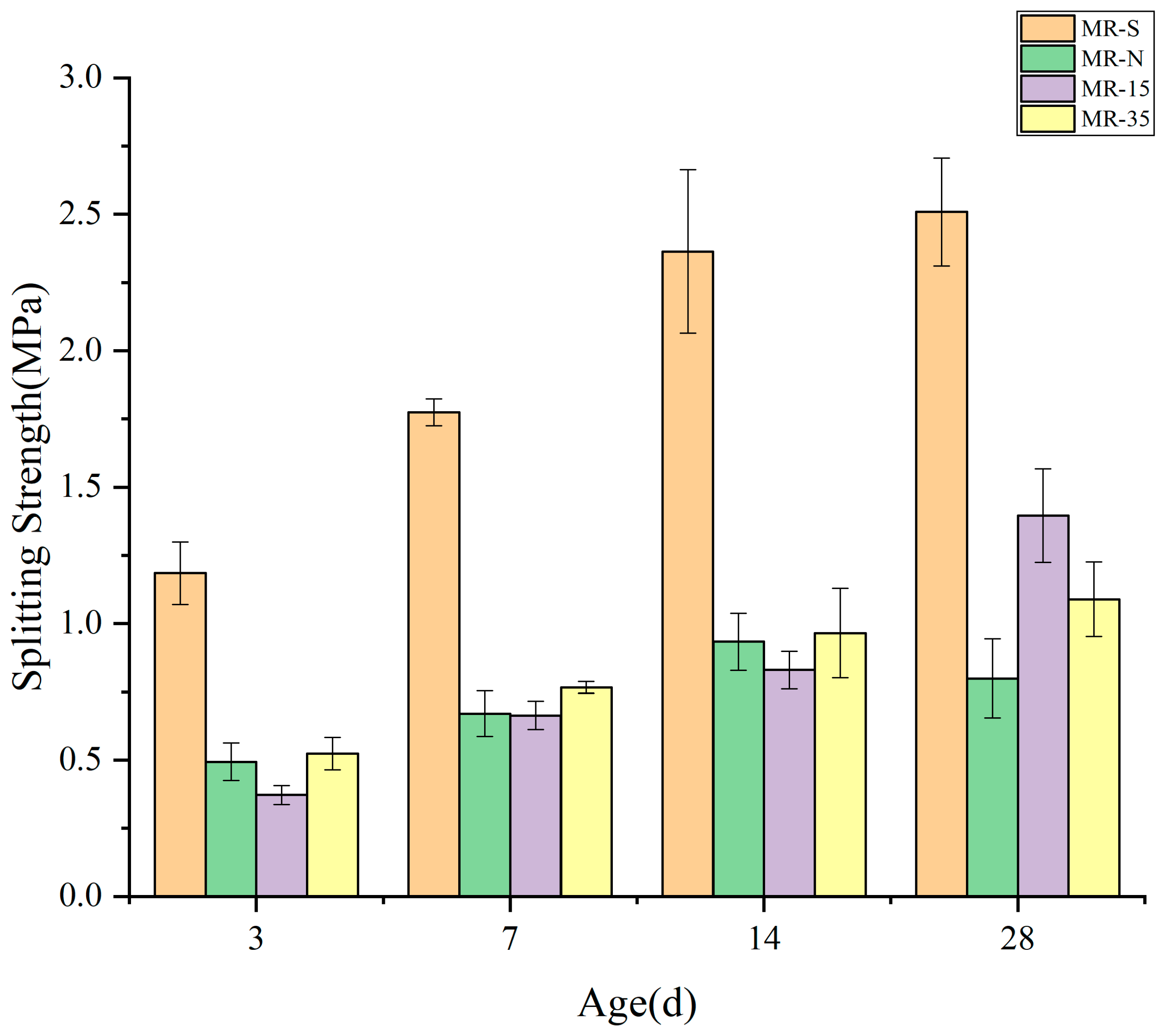
The relationship between different treatment methods, ages, and splitting strengths of the concrete junction is shown in Figure 8. When using same treatment method, the splitting strength of the concrete interface increased with age, and the growth rate was relatively slow. Only the unwashed treatment group had a slight decrease in splitting strength at 28 days. This showed that when the early-pouring specimen and the new specimen were used at the same time, the previous concrete specimen needed to be soaked in clean water. This affected the contact between new and old concrete specimens to some extent. If no corresponding treatment measures were taken, the contact between the concrete specimens would become worse after a period of time (28 days) and the splitting strength would be weakened. In addition, the splitting strength was related to the composition of cement. The late strength of cement would be reduced if the alkali content was too high. Admixtures could also decrease the late strength of cement, requiring additional experiments to prove the extent of the impact on the cement.

The splitting tensile strength of the integrally poured concrete (MR-S) was much higher than that of the layered concrete at all ages. It can be seen from the figure that at 3–14 days, the relationship of the splitting strengths of each treatment group was MR-S > MR-35 > MR-N > MR-15. At 28 days, the relationship between the splitting strengths of each treatment group was MR-S > MR-15 > MR-35 > MR-N. This was because the concrete specimens were not completely solidified at 3–28 days, and the splitting strength of different treatment methods was not obvious at 3–14 days. At 28 days, the splitting strength of MR-15 was higher than that of MR-35. A higher scouring strength made it easier to produce bubbles after the mortar was washed away, which would reduce the splitting strength.

3.3. The Relationship between Filling Volume, Average Amplitude, and Normal Angles Std. Dev.

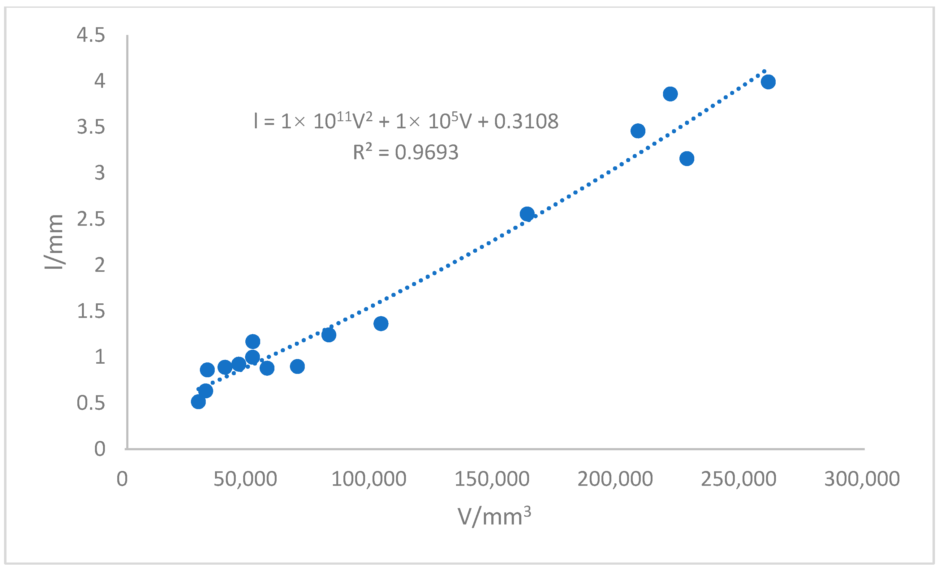
The average amplitude, normal angle std. dev., and filling volume were not the same. It was worth exploring what kind of relationship existed between them. From the results of this experiment, it could be seen that the larger the filling volume, the larger the mean amplitude, and the two were approximately quadratic, as shown in Figure 9.

Through mathematical regression, the relationship model between the mean amplitude l and the filling volume V could be obtained as follows, where the goodness of the regression fit was $R^2=0.9693$.

$$l=1E-11V^2+1E-05V+0.3108$$

(18)

The larger the filling volume was, the larger the normal angle std. dev. As shown in Figure 10, through mathematical regression, the relationship between the normal angle std. dev. and the filling volume was obtained. The goodness of the regression fit was $R^2=0.9324$.

$$\tau =-3E-12V^2+3E-06V+0.2097$$

(19)

From the perspective of mathematical regression, the normal angle std. dev. and the average amplitude can replace the filling volume as an index for evaluating roughness.

3.4. Relationship between Crackle Strength and Roughness

In the analysis in 3.1, the concrete had not completely solidified when the age was 3–14 days, and the splitting strength of different treatment methods was not obvious. Therefore, when analyzing the relationship between strength and roughness, we only selected the 28-day age. The data served as a reference.

Table 5. Pearson’s correlation test of the concrete splitting strength.

	V	L	s	τ	φ
$f_{ts}$	0.577 *	0.495 *	0.456 *	0.709 *	0.343

Two-tailed significance test. * indicator is significant at the 0.05 level.

showed the correlation between the five concrete roughness indices and the concrete splitting strength.

Table 5 shows that the splitting strength of concrete had a significant correlation with the concrete filling volume, average amplitude, surface area expansion rate, and normal angle std. dev. The normal angle std. dev. included angle was closely related to the splitting strength, and the filling volume also had a certain relationship with the splitting strength, while the relationship between the average amplitude and the surface area expansion rate and the splitting strength was relatively weak. Next, we would only study the relationship between the filling volume and the normal angle std. dev. with respect to the tensile strength.

Figure 11 shows the test results and fitting curve of the correlation between the splitting strength $f_{ts}$ and the filling volume V. The curve equation was as follows, and the goodness of fit was R² = 0.731.

$$f_{ts}=0.6861\mathit{ln}\left(V\right)-6.049$$

(20)

It can be seen from the figure that when the filling volume was less than 10,000 mm³, the growth rate of the splitting strength was relatively fast. Within this range, as the flushing pressure increased, the floating slurry and debris on the surface of the concrete could be washed away, and the coarse aggregate was continuously exposed, which effectively caused unevenness of the interface and a continuous increase in roughness. As a result, the splitting tensile strength increased rapidly.

When the filling volume was greater than 10,000 mm³, the growth rate of the splitting strength began to slow until it became flat. This was due to the further increase in flushing pressure; more sand and gravel were washed away, leaving bubbles and voids, but the splitting strength increased slowly or even decreased. In this range, although the filling volume continued to increase and the roughness continued to increase, the splitting strength was close to the extreme value, so the growth was increasingly at a slower pace. The fitting curve of the correlation between the splitting strength and the filling volume has a lesser R². This simply means that other variables that affected the dependent variable were missing.

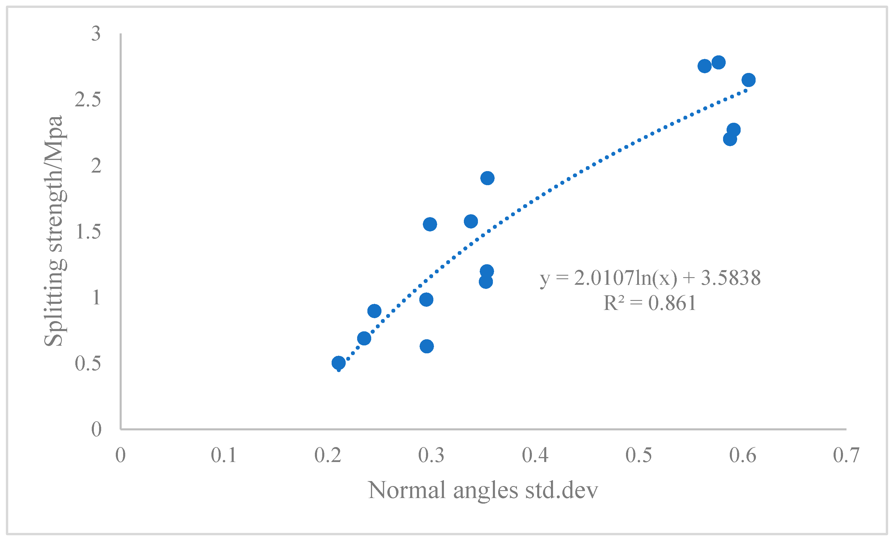
Figure 12 shows the test results and fitting curve of the correlation between the splitting strength $f_{ts}$ and normal angle std. dev. τ. The curve equation was as follows, and the goodness of fit was R² = 0.861.

$$f_{ts}=2.0107\ln \left(\tau \right)+3.5838$$

(21)

It can be seen from the figure that when the normal angle std. dev. was less than 0.4, the growth rate of the splitting strength was faster. When the normal angle std. dev. was greater than 0.4, the growth rate of the splitting strength slowed down. Figure 12 showed that the filling volume was closely related to the normal angles std. dev., which could effectively reflect the surface roughness of concrete. Comparing the fitting curves and correlation coefficients of the relationship between these two indicators and the splitting strength, the normal angle std. dev. could more significantly show the relationship with the splitting strength, and the degree of fit was higher.

4. Discussion

Using the “line” sampling processing method, the approach in this study was to select some straight-line segments on the rough surface. The polyline segment that characterized the surface information of the rough surface could be obtained by measuring the relative position of the points on these straight-line segments. Then, certain roughness parameters could be designed for calculation according to the characteristic points on the polyline segment. The mechanical stylus is a roughness measurement tool widely used in laboratory environments [33]. The measurement system mainly includes probes and mechanical advancers. To simplify the operation of the mechanical stylus, the profile texture meter has been invented [34]. Compared with the mechanical stylus, the profile texture meter is more conducive to the calculation of standardized roughness parameters. However, it uses photography methods to obtain polyline patterns, and its accuracy is limited by the camera’s imaging level and on-site lighting conditions. At the same time, because the probe’s free fall is dependent on gravity, it must be held vertically downwards and the rough surface to be detected must be kept horizontal, which can be difficult in practice. The PDI method has also been developed [35], but it is complicated to operate. It has a heavy workload and can cause irreversible damage to the rough surface. Therefore, although the PDI method is theoretically feasible and its accuracy is fully guaranteed, it is often not applicable in actual operations. None of these processing methods based on “line” sampling can guarantee complete randomness when drawing lines, and they can only minimize accidental errors through multiple tests. The accuracy of the detection results is poor, and the distribution of roughness on the plane will not be fully reflected.

The “surface” sampling method obtains roughness parameters by analyzing the rough surface as a whole or by sampling rough surface samples. Generally, compared with the “line” sampling method, the rough surface parameters obtained through the “surface” sampling method are more reasonable and accurate. A method based on “surface” sampling has higher accuracy than that based on “line” sampling because more combined surface information is collected and used for calculation. In the case of repeated sampling, the fluctuation of the detected results is smaller. The International Concrete Restoration Association (ICRI) proposed concrete surface profiles [36]. As a visual comparison method, this is simple to operate, and the detection time is short. However, the subjectivity of the detection personnel’s judgment in this method is difficult to avoid. Additionally, as a qualitative detection method, this method cannot provide accurate roughness detection values. Alternatively, the sand patch test is a method of quantitatively detecting roughness, which can calculate the average value of roughness in a certain area [8,37]. It is simple to operate and low in equipment cost, and it can be operated in prefabricated component factories or construction sites. However, the sand patch test requires that the surface to be tested must be kept level, which can add extra workload in actual operations, and it is difficult to maintain an absolute level. In addition, the presence of voids in the powdery material may affect the accuracy of the results and cause the rough surface to require secondary cleaning. The water accumulation method, which is similar to the principle of the sand patch test, can avoid the influence of the powdery material and the rough surface. However, because the concrete has a certain degree of water absorption, it is necessary to ensure the surface to be tested fully absorbs water before the measurement, and there should be no accumulation of water. This is difficult to control in actual operations, and the feasibility is not high. The slit-island method is similar to PDI and also theoretically feasible, but in actual operations, it can cause irreversible damage to the rough surface, and it has low efficiency and slow run times, which are not conducive to actual operations [38].

Compared with the above methods, the concrete bonding surface roughness detection method based on 3D laser scanning technology has the following advantages [16,39,40,41]: (1) The bonding surface to be tested does not have to be level. In fact, as long as the lighting conditions are good, 3D laser scanning technology can scan the joint surface to be inspected at any angle. (2) This method is a non-contact, non-destructive testing method. The material properties of concrete mean its surface can reflect the laser beam well so there is no need to preprocess the joint surface to be tested. At the same time, since there is no material contact with the bonding surface during the detection process, the bonding surface to be detected will not be damaged. As a result, no additional cleaning treatment is required after the detection. (3) This method is simple and practical. The accuracy of the results obtained by 3D laser scanning technology is high. Both the mean amplitude and the normal angle std. dev. demonstrated in this paper could replace the filling volume and improve the detection accuracy.

5. Conclusions

This study explored the feasibility of detecting the roughness of a concrete bonding surface using 3D laser scanning technology. To that end, we produced concrete test blocks with rough surfaces under different scouring pressures and conducted split tensile experiments. Through the analysis and discussion of the experimental results, the following conclusions were drawn:

(1) We used 3D laser scanning technology to detect the roughness of a concrete joint surface, and a point cloud correction algorithm was proposed, which we showed offers the possibility for handheld field measurement of roughness.

(2) This paper discussed the changes in the roughness of the concrete bonding surface under different scouring pressures. Overall, the indicators of the 35 MPa flushing treatment group were significantly higher than those of the other two groups. Except for the two indexes of surface area expansion rate and curvature std. dev., the values of other indexes in the 15 MPa treatment group were higher than those in the untreated group. As the flushing pressure increased, the surface roughness of the concrete also increased. This was in line with our first hypothesis.

(3) A corresponding relationship was established between the 28-day split tensile strength and the roughness index of the concrete specimens. Under the same treatment method, the splitting strength of the concrete interface increased with age, and the growth rate was relatively slow. When the specimen was less than 28 days old, the concrete specimen was not completely solidified, and the splitting strength was not obvious. A change model of the normal angle std. dev. and the split tensile strength was preliminary established, which provides the possibility for the direct evaluation of the concrete interlayer strength after the roughness is measured on-site in the future.

(4) The relationship between the split tensile strength of concrete and the roughness of the joint surface was discussed. The greater the roughness of the concrete bonding surface, the greater the split tensile strength. This was consistent with the second hypothesis to some extent. However, if the scouring pressure increased to a certain extent, this affected the structure of the concrete, thereby reducing the split tensile strength.

(5) By exploring the relationship between different roughness indexes, new evaluation indexes that could replace the traditional filling degree were found. The mean amplitude of the rough surface and the normal angle std. dev. could replace the traditional filling volume index, and the quantification effect was very good. Meanwhile, the correlation between the remaining index in the third hypothesis and the filling volume was not significant.