Article

Economic Land Utilization Optimization Model

1
Department of Construction Engineering, American University in Cairo, Cairo 11835, Egypt
2
Department of Architecture, American University in Cairo, Cairo 11835, Egypt
3
Horticulture Research Institute, Giza 12619, Egypt
4
Department of Computer Science, American University in Cairo, Cairo 11835, Egypt
*
Author to whom correspondence should be addressed.
Sustainability 2023, 15(3), 2594; https://doi.org/10.3390/su15032594
Submission received: 11 December 2022 / Revised: 22 January 2023 / Accepted: 24 January 2023 / Published: 1 February 2023
(This article belongs to the Special Issue Sustainable Buildings and Smart Cities)

Abstract

:
Recently, population growth and resource depletion have been matched by a growing demand for self-sustaining communities. Numerous studies promote sustainable solutions to the concerns of climate change and food scarcity. This study aims at creating an automated Economic Land Utilization Optimization Model (ELUOM) that identifies sustainable and cost-effective agricultural practices. Soil, water & climatic characteristics of over 400 crops are gathered in a relational database to build the model. Evolutionary algorithms are utilized to filter the database based on user input. Optimization process is then performed on all possible utilization plans of the filtered crops to maximize the 20-year return while minimizing water consumption. The model is verified on a case study in Giza, Egypt where it shows the potential of increasing the return/m3 of water by 370% versus current practices. This research also studies the application of ELOUM on a vacant plot in the American university in Cairo, Egypt.

1. Introduction

Increasing challenges of climate change, urbanization, and the depletion of non-renewable resources, necessitates the adaptation of innovative sustainable techniques in agricultural practices to satisfy the world’s growing demands. The interconnectedness between water, energy and food, accentuates the need to seek optimal tradeoffs between the three. In a domestic context, Egypt’s agriculture has recently become one of the most sensitive industries to the effects of climate change [1]. Current land utilization approaches neglect cost, energy, and water savings, which acts as an impediment to the establishment of sustainable and cost-effective green communities [2]. This research focuses on the water, energy and food nexus by designing a sustainable agricultural decision-making framework for the optimization of land utilization. The goals of this research are to: assemble a comprehensive database that links different crops to their cultivation requirements and to design and build an optimization model that formalizes potential uses for a plot of land. The Economic Land Utilization Optimization model (ELUOM) built by the research puts the database into application, which could result in a single use or multiple uses. Considering varying soil structure, topography, orientation, as well as client needs, the proposed framework optimizes land utilization to achieve minimized water demand and life cycle cost while maximizing the return on investment of the project. The proposed optimization tool can be considered a building block towards developing a water-energy-food nexus tool. A detailed description of the optimization model and how it operates is addressed through a study of various cases including the application of the developed optimization model on vacant land plots at the American University in Cairo (AUC) New Cairo Campus.

2. Literature Review

2.1. Currect Practice

Despite several individuals and organizations efforts, available agricultural crops databases lack comprehension. Whether directed towards specific climatic zone (ex. European Cooperative Program for Plant Genetic Resources database) or field specific databases, the available databases address single or few parameters related to crops and agricultural growth [3]. And although the United Nations Food and Agricultural Organization (FAO) provides a wealth of crop data, the information is dispersed over several databases and online platforms [4]. This highlights the need of developing a comprehensive database and integrating it in an optimization model that eases the decision-making process regarding agricultural land utilization. The model assesses efficient sustainable utilization for open field farming that maximizes return on investment.

2.2. Big Data and Sustainable Farming

Recently researchers and practitioners became interested in the integration of technology and big data in the agricultural sector. In 2015, Ryu et al., described an automated farming system, available on smartphones and tablets, that can be used to monitor and cultivate crops [5]. the research demonstrates the utilization of the Internet of Things (IoT) in measuring and controlling environmental parameters such as water, light, and temperature systems to provide the best growing conditions while reducing water use and carbon emissions [5].
Data-driven agriculture is a promising solution to solving the majority of the world’s food problems. And albeit the increased interest of big data utilization in agriculture, little research has been conducted on the topic of land utilization planning while the majority of research focuses on the monitoring and control of crops throughout the growing season [6,7]. In data-driven agricultural monitoring and control the main hurdles of smart farming application are found to be governance and data sharing legitimization concerns in a study done by Wolfert et al. [8]. However, in data driven agricultural land utilization planning, the main hurdle is the need for a comprehensive database for crops selection and agricultural cycle analysis. this research hence examines this gap and introduces a structured comprehensive that serves as the foundation for an integrated interface that helps users identify efficient and cost-effective approaches to utilizing a land plot for open field farming.

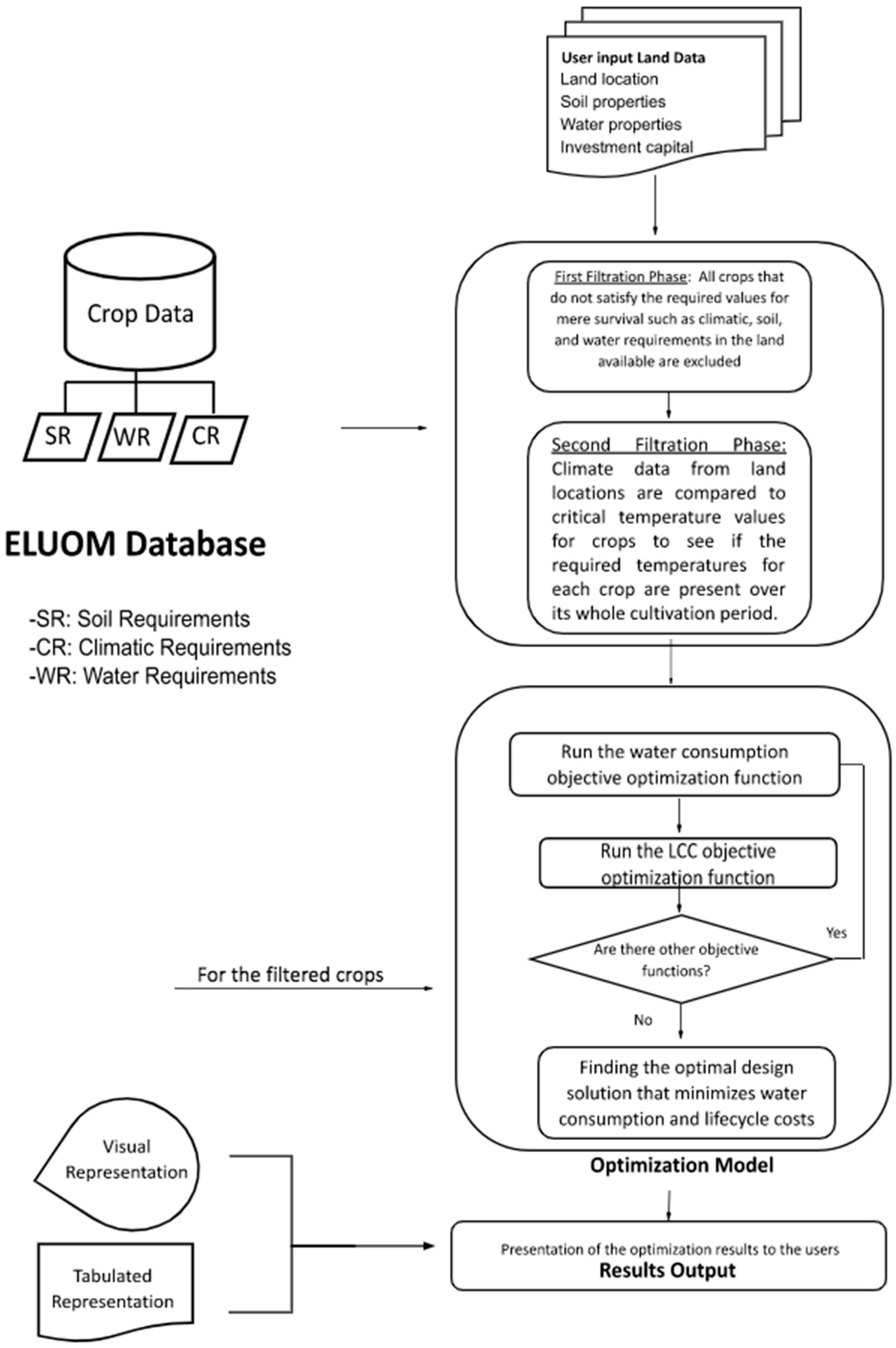
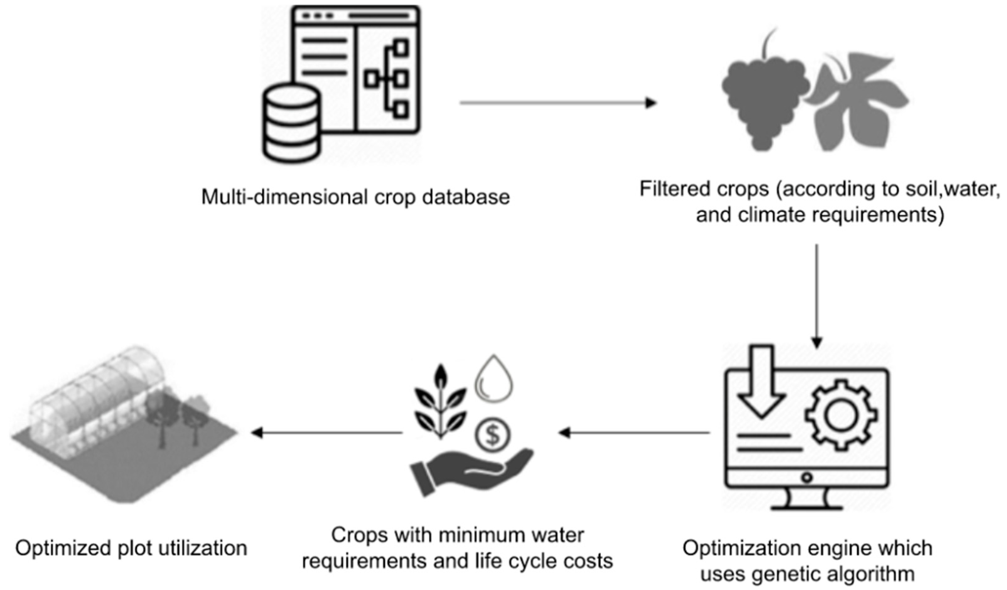
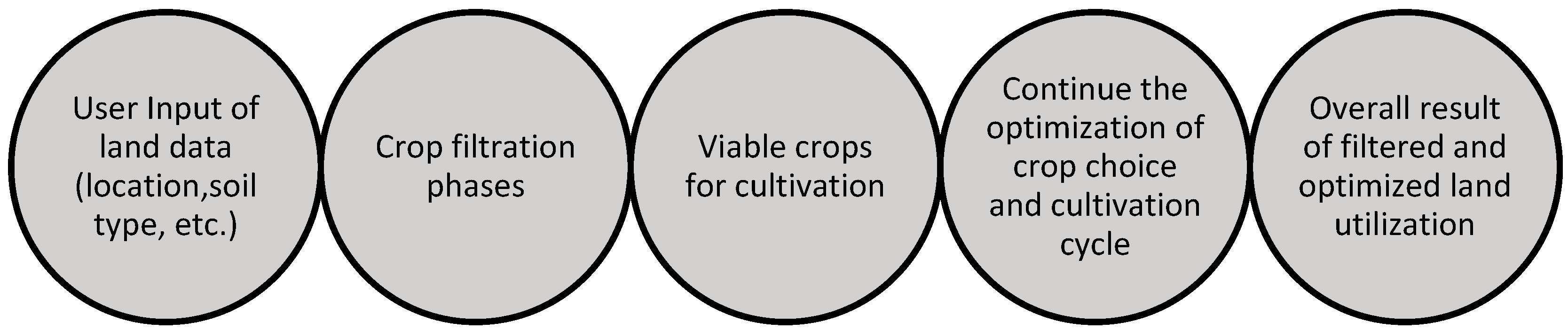
3. Research Methodology and Framework

The work on this project was divided into three stages, as depicted in Figure 1, the first stage is the knowledge acquisition. In this stage, interviews were conducted with professionals in the field of agricultural and sustainable development to identify all relevant information pertaining to the utilization of a land plot for farming functions. A synthesis of available scattered databases and best practices were analyzed and used to develop a relational database that links different plants and crops to their plantation requirements including soil, water and climatic needs. A comprehensive multidimensional database was assembled as the base of the automated optimization model which was then used to optimize the utilization of a land plot for farming and landscaping purposes while minimizing life cycle cost and water consumption. Stage two focused on the framework for the optimization model development where a set of algorithms were developed to produce an automated tool to support decision makers and landowners in selecting the crops to be cultivated in their lands. The third stage is the model validation and application. For the validation phase, the developed model was tested by inputting the data for a land plot in Giza that is currently being used for farming. The results of the model were then compared to actual crops currently being planted on that land to ensure the accuracy of the model outputs. The model was then sent to professionals in the field who tested the model and provided feedback on the model outputs and interface. Moreover, the model was applied on a vacant land plot at the American University in Cairo to provide the optimum land utilization scenario for the management of the university.

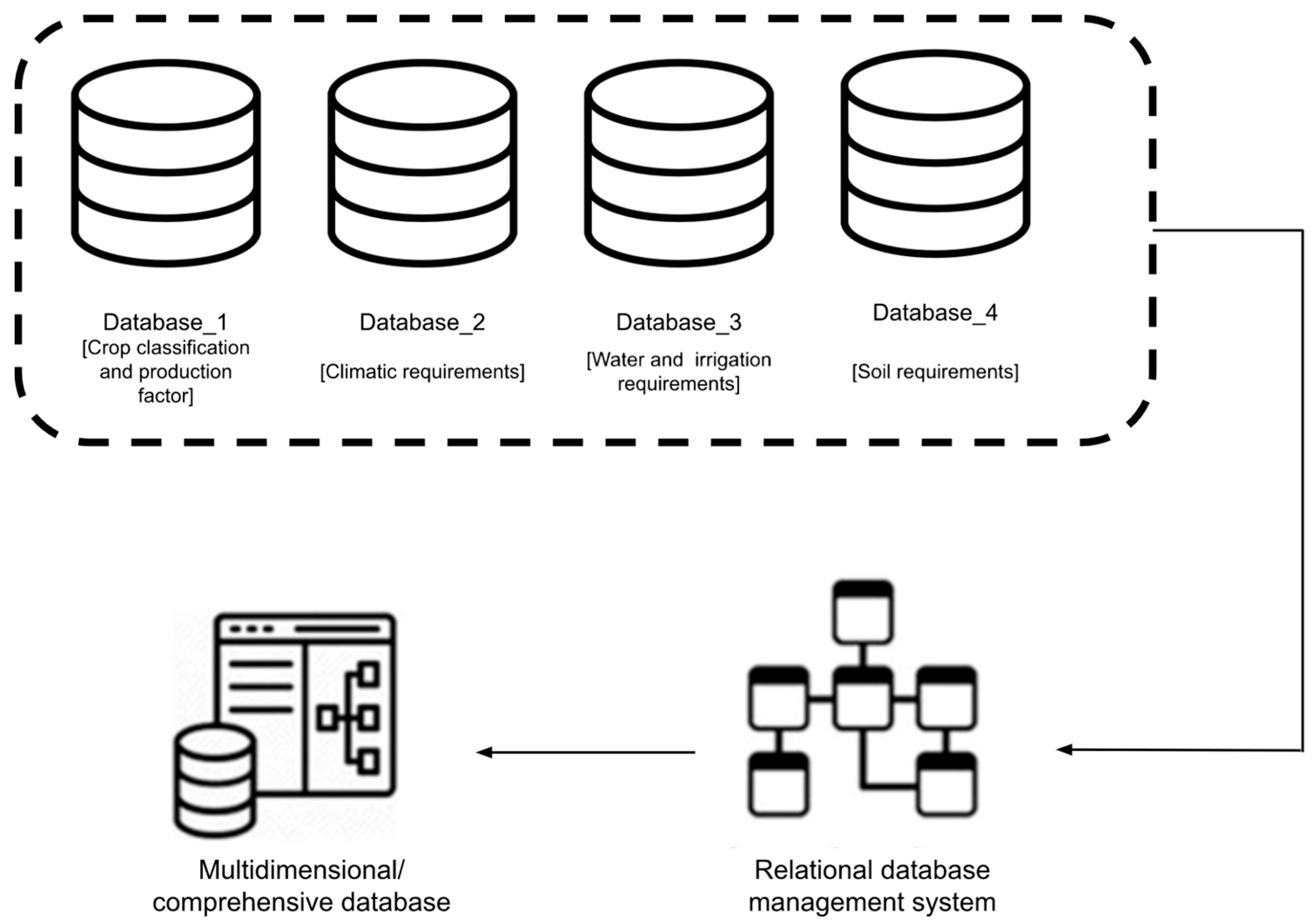
4. ELUOM Relational Database

Integrated in the ELUOM, is a comprehensive crop, as depicted in Figure 2. Field and literature research were done to gather and assemble data from multiple resources, including those provided by the FAO, in order to create the relational database. The crops database is intended to provide a thorough grasp of the crops’ features as well as the conditions required for their cultivation. This is accomplished by outlining a number of criteria that are either necessary for the crop’s cultivation or have an impact on its productivity. The crops database includes all the factors that can impact users’ crop selection which includes crop classification, soil parameters, water parameters, crop characteristics, irrigation systems, climatic circumstances, and production. The next section briefly explains the significance of each metric as well as its impact on crop production and yield. Detailed explanation of the crop selection criteria used in the construction of the database is described in Hosny et al. 2021 [9].

4.1. Crops Database

4.1.1. Crops Classification

In the database, the crops are classified based on their commercial name (the name commonly used in commercial products), the scientific name (the name in literature) and family classification which may vary to be either a fruit, vegetable, field crop, cereal, legumes, oilseeds, medicinal plants, herbs or trees. A crop can be classified under several families (ex. be fruit & a tree).

4.1.2. Soil Parameters

Another important consideration when choosing the correct crop for a given site is the soil type. Soil kinds are determined by the texture and organic matter content of the soil. Gravel, sand, clay, and silt, as well as peaty and loamy soils, are examples of soil types and textures. Soils are rarely made up of just one element or particle; they are usually made up of a mixture of sand, silt, and clay. Soil categorization goes beyond texture and particle size to include the presence of particular components in the soil as well as the soil’s salinity state. As a result, the database includes columns for listing each crop’s suitability in several soil types, including chalky soil, calcareous soil, saline soil, gypsum soil, and acidic soil. Each crop’s optimal and critical pH values are listed in the database. Increased exchangeable sodium levels can have a negative impact on the soil’s chemical and physical characteristics, ultimately harming plant growth [10,11]. Because excess sodium is related to calcium and magnesium, the impact of excess sodium and salinity in soil can also be assessed using the sodium adsorption ratio (SAR) [12]. The soil depth, which is defined as the distance from the soil surface to more-or-less consolidated soil layers [13,14], is another soil parameter included in the database. Soil drainage is stated qualitatively in the database, with the drainage requirement expressed either as well-drained soil is required or not specified. An average exchangeable sodium percentage (ESP) value along with the critical value for each crop is listed in the database. The level of ESP is associated with the relative ratio of Sodium and Calcium which is known as the sodium absorption ratio (SAR).

4.1.3. Water Parameters

The amount of salts present in both the water and the soil determines the electrical conductivity of the soil solution. Three electrical conductivity (EC) values are recorded in the database for each crop: the EC value advised for a 100% yield, the EC corresponding to 75% of the yield, and the critical EC value beyond which the crop does not live. Any agricultural operation relies heavily on water. The crop water needs, evapotranspiration (ET crop), is the quantity of water required for a crop to compensate for water loss owing to evaporation from the soil surface and transpiration from the crop during the course of its lifespan. Weather characteristics (ETO) and crop parameters are the two key factors that influence evapotranspiration (ET). Radiation, air temperature, humidity, and wind conditions all have an impact on the ETO value. The Kc (crop’s factor of evapotranspiration) value of each crop changes depending on the type and stage of growth. Irrigation water with a high salt content may cause salt to accumulate in the root zone [12]. Similarly, a sodium imbalance can impair crop yield. The term “sodicity” refers to a high salt concentration in irrigation water compared to calcium and magnesium, which reduces water infiltration [15]. While chloride is necessary for plants in small amounts, too much chloride in irrigation water can cause leaf burn when used with spray irrigation. Most plants are considered safe when chloride levels are less than 70 ppm. A quantity of more above 350 ppm, on the other hand, can be harmful to plant growth [15]. Similarly, boron is an essential element for plant growth. They are an impediment to optimal plant growth if present at very low concentrations [16], but higher concentrations greater than 2 ppm can be hazardous to some plants [12].

4.1.4. Crop Characteristics

The length of a crop growth season is the number of days when precipitation exceeds half of potential evapotranspiration [17]. It is calculated using a basic water balance model that links water availability to agricultural water demand using monthly figures [17]. The growth time of a crop has a significant influence on seasonal crop water consumption and crop cycle duration under typical circumstances, thus it is also tackled in the database [17].

4.1.5. Irrigation Systems

Another variable that is included in the database is the irrigation method. Each type of irrigation system has its advantages and disadvantages. Irrigation systems can vary in cost and labor input [18]. The suitability of the irrigation method depends on the local natural conditions (i.e., soil type, slope and climate), the type of technology used and the type of crops [18]. Thus, the database sorts the various types of irrigation methods including surface, sprinkler and drip irrigation based on the type of crops [18].

4.1.6. Climatic Conditions

Considering the climatic conditions, temperature plays a vital role in providing suitable conditions for optimum fruit production and maximizing fruit volume. The database will provide for temperature conditions suiting each type of crop. Suitability of temperature drives vegetative flushes with some crops and enhances fruit volume production with certain crop conditions [19]. Elevation affects crop production considering sunlight exposure angle, this reduced or enhanced light exposure may affect crop production volume and the overall biomass of plantation. The database however factors in recommended elevations for optimum crop growth and biomass results based on best practice and prior data reflecting favorable conditions for maxed out production.

4.1.7. Production Factors

Maximizing crop yield is one of the most important considerations. Preferred crops will need to have a large birth volume, with crop production being the determining factor in crop selection, especially in greenhouses with restricted space. The bigger the crop yield volume, the more cost savings may be realized. Crop density is an estimate of the number of seedlings to be planted inside a feddan based on real and standard practice-based data. Crop density will be crucial in determining which crop should be studied and factored in as a viable option. The majority of the literature depicted crop growing density as a range. The database’s ranges were determined by planting seeds.

5. ELUOM

5.1. Model Logic

There are three stages to the crop selection and optimization process. First, crops that do not satisfy the required values for mere crop survival in the available land conditions are excluded in the first filtration phase. The important survival factors are selected by agricultural specialists and are determined as follows:
Soil factors including:
soil type compatibility
ESP tolerance range
Acceptable minimum soil depth
and pH tolerance limits
Water parameters including:
crop’s maximum EC limit
chloride & boron content in soil
The second process is temperature & climatic conditions applicability filtration. In this phase, historical annual climate data from land locations is compared to critical temperature values for crops to see if the required temperatures for each crop are present over its whole cultivation period, and hence its suitability for cultivation. The third stage is optimization phase, where crops are evaluated in both economic & sustainable bases to determine the optimized crops combination that guarantees the highest economic return while minimizing water usage. Figure 3 details the decision flowchart of ELUOM.

5.2. Financial Data

ELUOM utilizes various economic factors in the optimization phase (third phase) to find the optimal crop combination and plantation cycle resulting in the highest return on investment. And because the financial part of any project is always one of the most determining variables in the end result, costs of all crops were gathered into a database incorporated in the model. The user can either enter or retrieve information on variable and fixed costs for setting up and operating open field farming from the databases. Crops costs were gathered from several sources, but the main one was official governmental reports detailing the crops costs in the entire agricultural sector in Egypt. These reports are produced on a yearly basis for a variety of common Egyptian crops that are distributed around the country. The reports are divided into two categories: summer crops and winter crops. The average yield output per feddan ( P r o k ) , and average cost per feddan ( I C C k ) of field crops are all included. A neural network approach was employed in the model to anticipate agricultural costs four years ahead of time by evaluating current economic conditions based on leading macroeconomic indicators. For each crop, a neural network model was created using the software Neural Designer, with economic indicators (World Bank indicators: Total reserves, Inflation, Exports of goods and services, GDP, Official exchange rate, and Agriculture, forestry, and fishing value added) as inputs and cost as output. There were 85% training cases and 15% testing cases in the model. The average total error in the test cases is 6%. After completing the four-year forecast, expert opinion was sought to generalize these costs to some other crops for which data were not available. The average increase in plant costs was used for other plants for which only one- or two-year cost data were available. Other data on harvest costs come from experts in this field with extensive experience in farmland and prices. Crops revenue per unit production is obtained through direct link with Egypt’s Obour market website; Obour market is the largest distribution market in Egypt, where farmers sell their produce to distributors who cover all over the country. The Obour market website is updated daily to reflect the selling price variation in the country mainly due to crop availability and season change. Figure 4 shows the various phases that the Integrated Optimizer goes through before reaching optimized land use results.
Similarly, operating costs such as land rent, maintenance, labor, water consumption, and harvester operation are included in the calculation. Users enter land rent along with prices for maintenance, saplings, pesticides, fertilizers, compost and equipment. For water and energy, the user only enters the price per m3 or KW.hour for the selected plant. The amount of water and energy required for each crop is already included in the database. Such information is obtained from previous literature and research conducted on national and international industry professionals. The net present value of the filtered alternatives, as well as the internal rate of return are calculated. The study period was chosen to be 20 years. Further elaboration on the optimization model is tackled in Hosny et al. (2022) [20].

6. Model Mathematical Formulas

All crops in the database take the notation i in the first filtration phase. Valid crops in the first filtration then take the notation j in the second filtration phase. Once all crops finish the filtration phases, the valid crops then proceed to the optimization phase; where they are given the annotation k . There are n i number of crops, n j number of crops j , and n k number of crops k .

6.1. First Filtration Phase

For a crop to be selected in the initial filtration Phase, it must satisfy the following conditions:
(1)
Soil Parameters
Soil type compatibility requirement
Exchangeable Sodium percentage Requirement
Soil Depth requirement
pH requirement
(2)
Water Parameters
Water Ec requirement
Chloride requirement
Boron requirement
The following section explains in details each parameter and the related equations.

6.1.1. Soil Parameters

Soil Compatibility

Soil compatibility is essential for the survival of the crop. In the database, the main types of soil are listed as follows: Sand (Sa), Silt (Si), Clay (Cl), Limestone (Li), and for each crop a value of either 0, or 1 is listed under each soil type indicating if the crop survives in the specific soil type. The crop’s soil matrix is multiplied by the given field matrix Equation (1); where a value of 1 is obtained if the crop is suitable for the type of land (field).
For n   N u m b e r   o f   C r o p s :
C r o p i   S o i l   M a t r i x     f i e l d   M a t r i x = 1
S a i S i i C l i L i i 1 0 0 1 S a f S i f C l f L i f 1 0 0 0 = [ 1 ]
Subject to:
Soil Matrix Contains Soil Types: {Sai, Sii, Cli, Lii} = {Sand, Silt, Clay, Limestone}.
Field Soil Matrix Contains Types: {Saf, Sif, Clf, Lif} = {Sand, Silt, Clay, Limestone}.

Exchangeable Sodium Percentage

Exchangeable Sodium Percentage must be within crop survival limits as demonstrated in
ESPL,i < ESPf < ESPU,I
where ESPL,i: ESP lower limit suitable for Crop I; ESPU,i: ESP upper limit suitable for Crop I; ESPf: ESP value for the field.

Soil Depth Requirement

Minimum soil depth for crop i growth must be satisfied. This is illustrated in Equation (3)
Dmini < Df < Dmaxi
where: Dmini: Minimum soil depth suitable for Crop I; Dmaxi: Maximum soil depth suitable for Crop I; Df: Actual soil depth in the field.

pH Requationuirement

Land pH level must be within the upper and lower limits of crop i as illustrated in Equation (4)
pHL,I < pHf < pHU,I
where: pHL,i: pH lower limit suitable for Crop I; pHU,i: pH upper limit suitable for Crop I; pHf: pH level in the field.

6.1.2. Water Parameters

Electric Conductivity (EC)

Irrigation Water Electric Conductivity (EC) must be less than that of the maximum tolerated level of crop i ; which is illustrated in Equation (5)
ECwf < ECwi
where: ECwi: Maximum EC water suitable for Crop I; ECwf: Available Irrigation water’s EC.

Chloride Level

The chloride level in the field must be less than the maximum tolerance level of crop i , This is illustrated in Equation (6)
C L f <   C l i
where: C L f : Chloride level in the field; C l i : Maximum Chloride level that crop i can withstand.

Boron Level

The Boron level in the field must be less than the maximum tolerance level of crop i , This is illustrated in Equation (7)
B r f < B r i
where: B r f :Boron Level in the field; B r i : Maximum Boron level crop i can survive.

6.2. Second Filtration Phase

All crops selected from the first filtration phase take the notation j and are filtered in the second phase based on temperature and climatic condition, eliminating the unfit crops to survive in the given land surrounding climate.

6.2.1. Filtration Logic

This filtration phase is for temperature; where crop j is valid if the crop’s survival temperatures are not violated for a consecutive period of time that is equal to or greater than the minimum time the crop needs to grow and reach yielding. This is expressed by the following equations:
For j = 1 to j = nn
Crop   j   is   valid   ( passes   the   filtration   phase )   if   TVmfj   > P S D j
where: P S D j :Average production season duration that crop j needs to start producing.
TVmfj = is the largest consecutive sum of TVm,j
T V m , j is defined as follows:
{ f o r   m = 1   t i l l   m = 12 , T V m , j = 1 , ( T L , j , f - T A L > = T L , j ) & ( T U , j , f + T A L > = T U , j ) , T V m , j = 0 , O t h e r w i s e
TAL is defined as follows:
{ CCj : = Tree ,   TAL = 5 ° ,   CCj : = field ,   TAL = 2 °
where: TL,j: Minimum Temperature (celsius) that crop (j) can withstand; TU,j: Maximum Temperature (celsius) that crop (j) can withstand; TVm,j: Temp Validity for crop j in month m (Binary Value); TAL: Temperature sensitivity allowance based on crop classification; CCj: Crop Classification for crop j that can take only one value of the following: (Tree or open field).

6.2.2. Second Filtration Phase Output

If the window of temperature validity for crop j is greater than the Average production season duration that crop j needs to start producing (When TVmfj > P S D j ), then there becomes a range of time in which we can start cultivating and harvesting. In this case crop j does not have to start at a certain month but rather in a month within a range and this value is variable m k .
Yet m k is guided by a window of temperature validity by upper and lower limit (months) that the crop can be cultivated to allow for enough time satisfying the P S D j duration within acceptable temperature conditions for crop j . For each valid crop j , the following values are calculated from the second phase filter:
m l k : lower limit of the cultivation period in months of crop k; the first month that crop k is valid to be cultivated.
m u k : Upper limit of the cultivation period in months of crop k; the last month that crop k is valid to be cultivated to have enough valid time before yield.

6.3. Optimization

All valid crops, passing the first & second filtration phases, are elected for the optimization module and are given the annotation k . The optimization process is defined by three attributes: the objective function, constrains, and variables of optimization. The Optimization process is done using a genetic algorithm utilizing Excel Evolver Add-in. This section explores the attributes defining the optimization module in detail.

6.3.1. Variables

Proper land cultivation is planning which crop to be planted during what time, and in the case of multiple crops the area of the land that each crop should utilize. These kinds of information are the variables in the optimization module which are divided into two sets of variables. The first is related to the area to be planted from selected each crop, while the other is related to the cultivation starting month for each crop k .
Variable set 1: n k   n u m b e r   o f   m k   V a r i a b l e s
Subject to:
m l k m k m u k
where: m k : Starting cultivation Month of crop k; m l k : lower limit of the cultivation period in months of crop k; the first month that crop k is valid to be cultivated. m u k : Upper limit of the cultivation period in months of crop k; the last month that crop k is valid to be cultivated to have enough valid time before yield.
Variable set 2: n k   n u m b e r   o f   A c k   V a r i a b l e s
Subject to:
A c k > 0 ; A c k A M , & A c k A T
where: A c k : Area cultivated from crop k; A M : M a x i m u m   A r e a   p e r   c r o p   ( U s e r   D e f i n e d ) ; A T : Total Land Area

6.3.2. Constraints

There are several constraints guiding and limiting the optimization process. These constraints cover logical constraints, Budget limitation, Water & land availability limitations, and some user preferences guiding the solution. Below is a list of all constraints with their mathematical representation
Constraints:
  • Sum of feddans to be planted should be equal or less than total land area for each month
  • Sum of feddans planted per crop should be equal or less than maximum area allowed per crop (if determined by user)
  • Sum of number of crops to be planted should be equal or less than Maximum Allowed no. of crops to be planted in a land (user determined)
  • Sum of water needs for crops to be planted should be equal or less than maximum available water per day
  • Sum of costs needs for crops cultivation & Greenhouse construction & operations should be equal or less than maximum available capital
  • Land Availability Constraints
Sum of feddans to be planted should be equal or less than total land area for each month.
f o r   e a c h   m o n t h m A T > = A C , m
where: A T : Total Land Area; A C , m : Cultivated Area of the Land in month m.
2.
Water Availability Constraint
Sum of water needs for crops to be planted should be equal or less than maximum available water
W T > k = n k = 1 W C k / 365   D a y s
where: W T : Total Daily Water Available; W C k : Yearly Water demand for crop k ( m 3 / y e a r ).
W C k = m = 12 m = 1 [ E T o / m o n t h K c k N o . D a y s / m o n t h A c k ] / [ 1000 I r r i g a t i o n   W a t e r   E f f i c i e n c y ]
where: E T o : Evapotranspiration (mm/day) based on weather conditions for land location; K c k : Crop Factor of evapotranspiration for crop k; A c k : Area Cultivated of crop k in m2.
3.
Crop Area User Limitation Constraint
Sum of feddans planted per crop should be equal or less than the maximum area allowed per crop (if determined by user). The user can determine in integers the maximum number of feddans to be planted by a single crop.
A c k < = A M
where: A c k : Area cultivated from crop k in feddans; A M : Maximum Area per crop (User Defined).
4.
Crop Variety User Limitation Constraint
Sum of number of crops to be planted should be equal or less than Maximum Allowed no. of crops to be planted in a land (user determined)
N c < = N M
Subject to
f o r   k = 1   t o   k = n , N c + + , ( i f A c k > 0 )
where: N c : Number of cultivated crops with initial value of 0; N M : Maximum number of different crops to be cultivated defined by user.
5.
Budget Availability Constraint
Sum of costs needs for crops cultivation should be equal or less than maximum available capital
I C < = I I
I C = I C f + I C G H
where I C : Initial cost of cultivation of optimized crops (inclusive to all) in EGP; I C f : Initial field crops/trees cultivation cost in EGP; I I : Initial Maximum Investment value/Available Capital (User defined) in EGP.
I C f = k = n k k = 1 I C C k A c k , I C C k
obtained as explained in Section 5.2
where: A c k : Area cultivated from crop k in feddans; I C C k : Initial field cost per feddan for crop k in EGP in year of simulation.

6.3.3. Objective Function
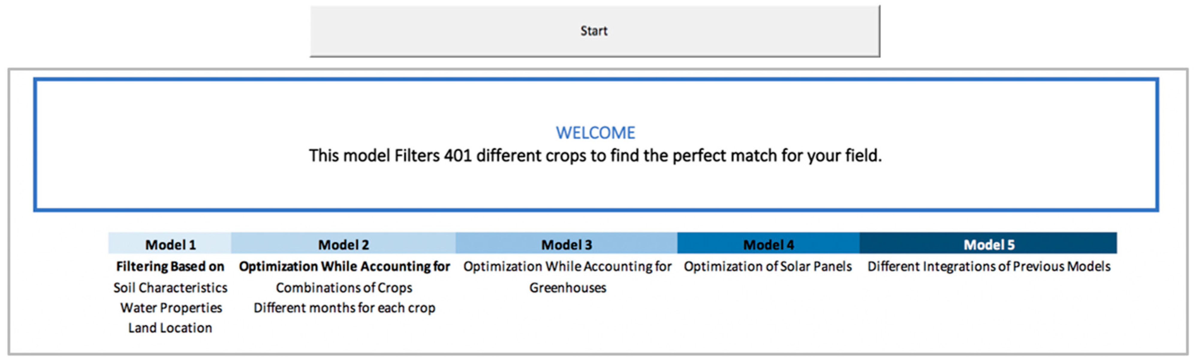
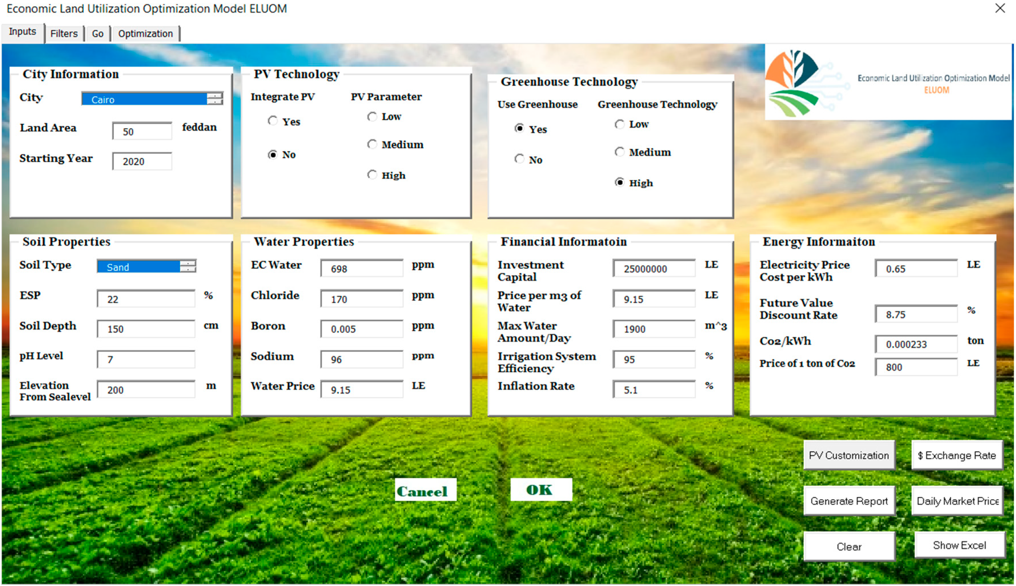
The objective function of ELOUM is concerned with maximizing the Net present value of 20-year cash flow.
Maximize   y = 20 y = 1 N P V ( R y ) = R y ( 1 + r ) y
where: N P V : Net Present Value; R y : net cash flow at year y ; r : annual interest rate (User defined or set according to Egypt Central bank); y : number of periods interest held (years).
R y = A c k ( R e v k P r o k ) - I C C k
where: A c k : Area cultivated from crop k in feddans; R e v k : Revenue of one production unit of crop k obtained from Oboor market P r o k : E x p e c t e d   p r o d u c t i o n   q u a n t i t y   p e r   f e d d a n   o f   c r o p   k ; I C C k : Initial field cost per feddan for crop k in EGP in year of simulation.

7. Model Interface

In order to commercialize ELOUM, a Graphical user interface is developed to ease the user’s experience. ELOUM package is easily downloaded on any computer with easy steps for installation. The model utilizes excel-based visual basic and python code in the development of the user-interface. Upon installing and running the automated interface for “ELUOM,” i.e., Economic Land Utilization Optimization Model, the user is met with the homepage as shown in Figure 5.
The user has then to input details related to the location of the land plot, soil and water properties. Budget constraints, water and energy prices can be also inserted in the model at this stage. Figure 6 showcases the steps that the user has to go through to reach the optimized output for land utilization. To better illustrate the end user journey, the process is applied through the case studies presented in the next section.

8. Model Validation and Verification

8.1. Overview

In order to validate the filtration process, a case study of an agricultural land in the Qata area of Giza, Egypt is used. The land area is 30 feddan, and the soil is largely sandy, with an ESP of 10% and a depth of 1000 cm. The landowner grows cucumber and peas in multiple cycles. The EC of the water is 450 parts per million, whereas the contents of chloride, boron, and sodium are 350 parts per million, 1.2 parts per million, and 3 parts per million, respectively. The data presented is based on existing land practices and real numbers from the Giza Land. Domestic water costs 1.5 Egyptian pounds per cubic meter. Several financial characteristics, such as the 50,000.00 EGP per feddan investment capital for utilizing this specific land piece suitable for agriculture, were used to assign investment capital. The is cultivated by the owner, and hence the land rental amount was not applicable. Based on current labor prices, the cost of a work man hour ranges between 20.00 and 25.00 EGP. The landowners provided an electricity tariff/kWh based on the irrigation class rate of 0.65 LE. Based on national figures published by the Central Bank of Egypt, a 5.1% inflation rate was utilized to reflect the average rate in Egypt during the last several years.

8.2. Current Agricultural Practices at Giza Land

Looking at the financial cycle of the land, it is clear that the landowners were targeting a short-term profitability that limits the use of their capital. The owners, although have on hand 1.5 million EGP as investment capital, chooses to invest roughly 0.6 million EGP in short term crops, see Table 1. This is because these crops provide a fast turn over and require a low initial capital investment. Currently the landowners plant cucumber and peas in the summer and winter for the variation of crops with the season, see Table 2.

8.3. Model Validation

The Giza Land case study information was inserted into the model via the user interface. Sixty-five different crops suitable for cultivation on this land location are the result of the initial filtration step. After applying the temperature filtration (second filtration phase), 23 different crops are determined to be suitable for cultivation, demonstrating the database’s functionality. Peas and cucumbers are among the filtered crops presently being produced on the land, demonstrating that the results of the filtering operation are consistent with real life practices achieving validation. The large number of crops that have been confirmed to be suitable for cultivation demonstrates the immense potential of employing optimization to help farmers and landowners get the most out of their land.

8.4. Model Optimization Verification

After performing the filtration phases, optimization is performed on the filtered crops to reach a near optimum solution that yields the highest profitability utilizing a low water consumption while maintaining all constraints. When the optimization module is implemented on this case, the model suggested a better alternative in terms of both water consumption and the NPV of the land in the long term. Instead of targeting short-term turnover and saving on the initial capital investment (current land owner practices), the model suggests utilizing almost all of the available funds into a variety of both long-term crops (trees & palm trees) and short-term ones (Less than a year crops). Four crops were selected out of the 23 crops that went through optimization, from which two crops are trees and the other two are field crops. This combination shows how the land is utilized to a great extent while using all the available capital and meeting all the constraints imposed through water requirements or plot area. The result of the model is to utilize the land in planting the following crops: sweet potatoes, beets, lemon trees, and bananas. Table 3 shows the distribution of the plants over the period of a year and the land utilization percentage. The results of the recommended management practices are summarized in Table 4.

8.5. Results & Discussion of Current Versus Recommended Agricultural Practices

The optimization model has led to a great increase in the expected financial return while maintaining a low water quantity usage. All of the model constraints were met, and the land area utilization percentage was maintained above 60%. The optimum solution that ELOUM generated yields an increase of NPV of 290% compared to current landowner practices. The analysis shows that with the current landowner approach the NPV/Initial Capital investment approximately gives 9.19 EGP for every 1 EGP of capital invested. The optimized scenario estimates the NPV/Initial Capital investment value to be 12.35 EGP for every invested 1 EGP. With the same budget, the user may have selected to plant less feddans of the crops chosen in the optimization phase allowing him to generate more profit from the same initial investment whilst lowering the water consumed and percentage of land utilization giving room for other kinds of investment. Also, the analysis demonstrates to the user how tripling his initial investment will affect his profits over a period of 20 years which should provide support to the user in taking the decision to aim for long term investments to maximize his profits. Overall, with regard to the Giza land, the model is effective in verifying the correctness of the data, and in enhancing the agricultural practices’ return and the land performance. Table 5 summarizes the comparison between current practices and ELOUM agricultural practice.

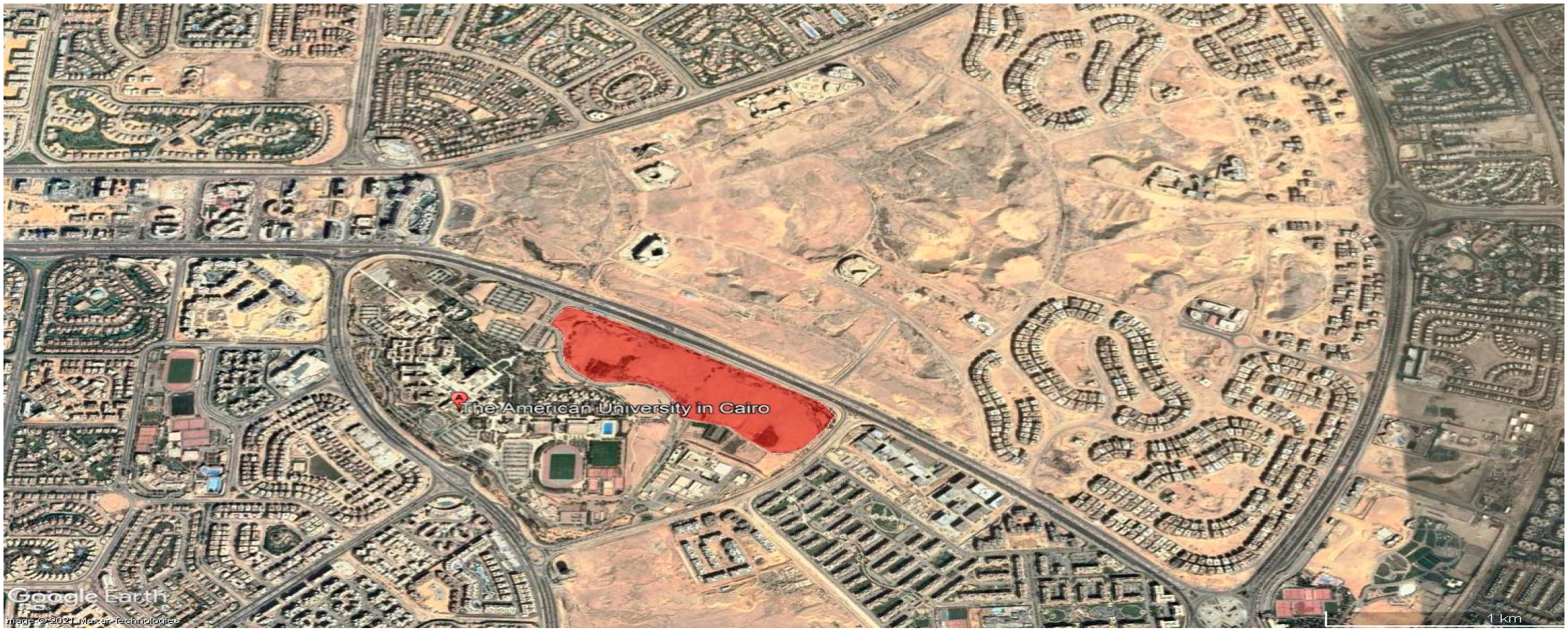
9. Case Study Application

9.1. Overview

The proposed ELOUM optimizer is used to suggest the potential optimum utilization for the available vacant land at the American University in Cairo for open field farming. The study area indicated in Figure 7. in red is approximately 50 feddans. The optimizer cross matches information provided such as land area, soil properties, climatic zone, current market price, operation costs and initial budget with data from the database to present the optimized solutions for land utilization that minimizes the life cycle cost and maximizes the return on investment. This entailed identifying crops that best match the available growing conditions while ensuring minimal water and resources consumption. The aim of utilizing ELOUM model on this case is to support the University’s vision and mission in continuously promoting and pioneering sustainable development and finding solutions to the challenges that climate change, food and resources depletion present.

9.2. Data Input

Soil and water properties along with some financial parameters are entered into the model Figure 8. The soil in this location is composed of sand, silt, clay and limestone. The soil ESP is 20% and the depth of the soil ranges from 0 to 1.5 m with an elevation of 200 m above sea level. Moreover, the pH level is between 7 and 8.5. Meanwhile the water parameters inserted into the model includes the ECw value, which is 1.09, Chloride (ppm) 170, Boron (ppm) 0.005, Sodium (ppm) 96. The maximum available water for irrigation is 1900 m3 /day with 95% irrigation system efficiency. The information provided is based on the campus irrigation consumption data over the past 7 year. While the cost per m3 of domestic water is 9.15 EGP, the cost of the treated wastewater is 3.60 EGP. Several financial parameters such as the 50,000.00 EGP per feddan allocated investment capital for utilizing the land plot. The cost of labor man hour is between 20.00 to 25.00 EGP, based on labor costs for other ongoing farming projects on campus. Electricity Rate was obtained based on the irrigation class rate to be 0.65 LE/kWh from AUC Administration. Inflation rate of 5.1% was used reflecting the average rate in Egypt in from the year 2016 till 2020 based on the national statistics provided by the Central Bank of Egypt and the Future Discounted Rate was determined to be 8.75% also based on the national statistics of the Central Bank of Egypt.

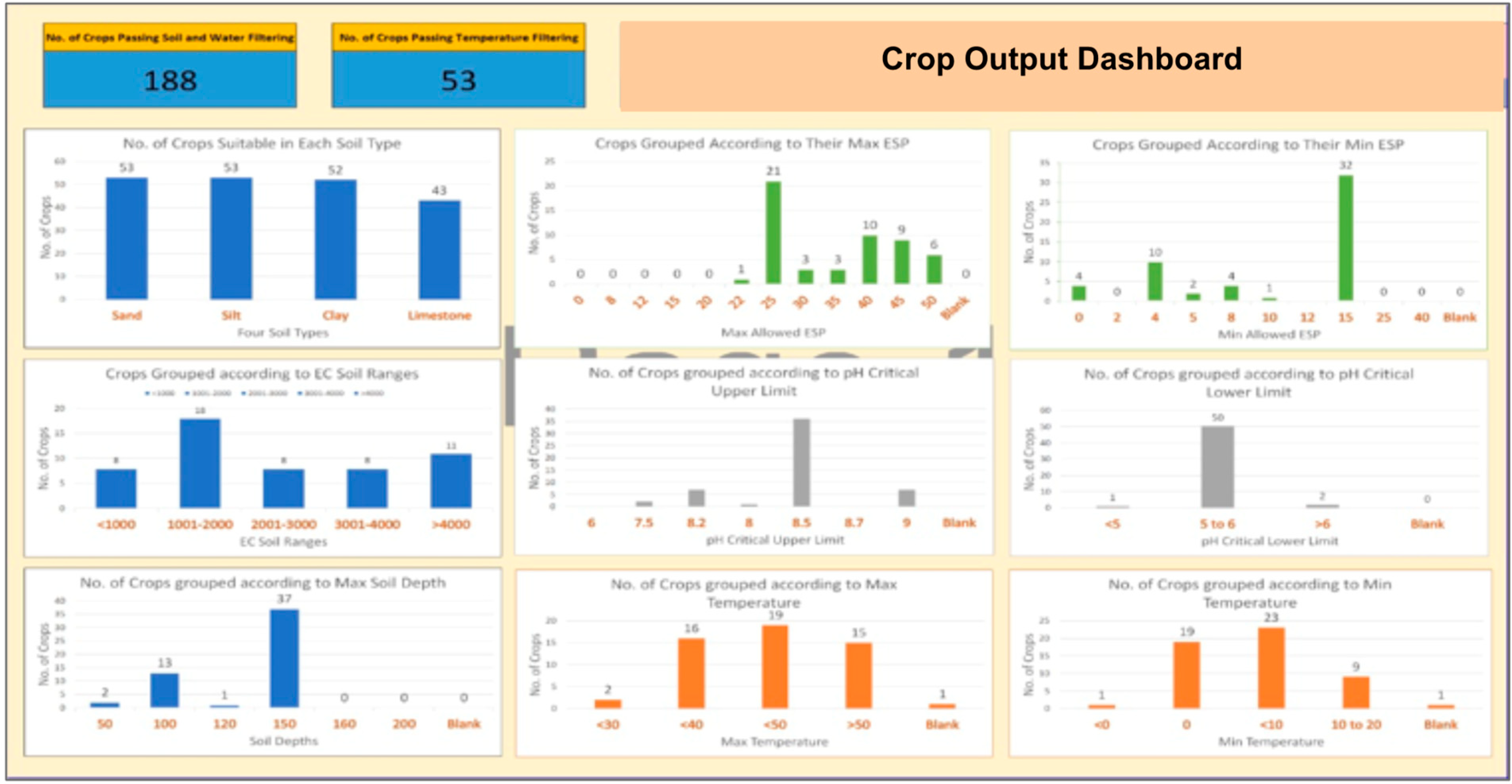
9.3. Filtration Phase

The Filtration Phase shows how 188 crops were suitable for the land without considering the temperatures; however, only 41 crops are suitable for the land location based on the climate condition in the area. The 41 crops included 17 field crops and 24 trees; indicated in Table 6.

9.4. Optimization Phase Result

The optimization process focused on reaching the highest net present value NPV for the land for the period of study (20 years) while minimizing the water consumption, see Figure 9. The result of this was to fully utilize the land by planting 6 different crops varying from trees and field crops. All capital, and minimum land utilization values were met. Table 7. shows a one-year crops cycle of the land, while Table 8 summarizes the expected results from the model, featuring roughly 72 M EGP as the 20-year NPV for an initial investment of 2.45 M EGP. The Model used an evolutionary algorithm to solve the optimization problem and was operated for more than 100,000 Trials reaching the shown solution.
The dashboard in Figure 9 summarizes the main characteristics of the filtered crops allowing the user to easily observe the majority of crops in each characteristic as to observe how the change in any of the characteristics will impact the pool of crops from which he/she is selecting. The characteristics show the soil, water, and temperature conditions available in the case study land plot that limits the crops suitable for cultivation. Also, the dashboard aids the user in reevaluating the values that he provided for each characteristic as he is able to observe if any of the values is not consistent throughout the cultivation process how many crops may turn to be unsuitable for his land and thus affects the expected yield.
Accordingly, the model suggested a combination of crops varying between field crops, trees, and palm trees. The suggested agricultural practice for the AUC plot was planting 20 feddans of lemon trees and 10 feddans of Bananas, having 0.85 of a feddan of Date palm trees, and having the remaining 29.1 feddans in a field crops rotation throughout the year as shown in Table 7. This allowed for short term gains as well as long-term gains and utilized the land entirely with a very low water consumption. The expected daily water consumption of the 50 feddans equates to 1126 m3/day. The low water usage combined with the high expected return on investment expected even from the first year, reflect the model’s ability to enhance the agricultural field. Figure 10. Exhibits the expected cash flow throughout the project 20-year period of study.

10. Conclusions and Recommendation

This study presents the framework for designing a state-of-the-art automated optimization model with a comprehensive database for optimizing land utilization for open field farming titled “ELUOM”. The automated model was created to fill a need in the industry for comprehensive crop datasets and multi-objective land usage optimization models. The research also demonstrates how comparable optimization techniques may be used to a variety of land plots, including undeveloped land on the AUC New Cairo campus planned to be used for agriculture. The automated interface was able to narrow down the crop choices to those with the lowest water and life cycle costs while increasing the project’s return on investment. This not only aids in the early planning of agricultural operations, but it also aids in overcoming the traditional instinctive process of deciding how to use a plot of land, which does not always produce the best or most sustainable return.
Despite its acknowledged potentials, the optimization model’s extensive relational database present limitations are that the growth duration period for crops included in the model is an average value, however the growth duration period should be per hardiness zone for more accurate results. ELOUM model also has a significant limitation of only considering traditional agricultural practices and not including Greenhouses cultivation practices which can significantly overcome natural land limitations in terms of climate conditions. It is recommended that the model integrates greenhouses crops and to cover an inclusive view of the different levels of technology of greenhouses. The model can also incorporate wide scale simulation allowing the scope of the research to expand using HYDRUS model [21]. In future revisions of the model, the user may be able to specify which objectives he or she wishes to optimize for. More data regarding crops that might grow in other countries could be added in the future. This allows the model to expand into international markets. Additional features, such as the inclusion of crop photos, will aid in the better display of model results.
To summarize, the optimization model demonstrated in this study is an example of how incorporating technology into farming and landscaping can aid in the sustainable management of available land and the expansion of green communities in the region, while bridging the gap between multiple industries and fields such as data analytics, project organizational management, and agronomics.

Author Contributions

Conceptualization, O.A.H., E.M.D. and K.A.T.; methodology, O.A.H., E.M.D. and I.A.; software, Y.H.; validation, H.K.G. and M.F.; formal analysis, Y.A.E.R. and A.S.; investigation, M.A., H.K.G., M.F.; resources, A.E.E.; writing—original draft preparation, M.A., H.K.G. and M.F.; writing—review and editing, E.M.D. and I.A.; supervision, O.A.H.; project administration, O.A.H.; funding acquisition, O.A.H. and K.A.T. All authors have read and agreed to the published version of the manuscript.

Funding

This research was funded by the Bartlett Fund for Critical Challenges grant number SSE—Construction—O.H—FY19—FY20 and the APC was funded by authors.

Institutional Review Board Statement

Not applicable.

Informed Consent Statement

Not applicable.

Data Availability Statement

No new data were created or analyzed in this study. Data sharing is not applicable to this article.

Conflicts of Interest

The authors declare no conflict of interest.

References

  1. McCarl, B.; Musumba, M.; Smith, J.; Kirshen, P.; Jones, R.; El-Ganzori, A.; Ali, M.; Kotb, M.; El-Shinnawy, I.; El-Agizy, M.; et al. Climate change vulnerability and adaptation strategies in Egypt’s agricultural sector. Mitig. Adapt. Strateg. Glob. Chang. 2015, 20, 1097–1109. [Google Scholar] [CrossRef]
  2. Hosny, O.; Dorra, E.; Tarabieh, K.; Nassar, K.; Zahran, S.; Amer, M. Quantifying the Social Impact of a Pilot Sustainable and Environmentally Friendly Optimizer for Urban Landscaping (SEOUL). In Proceedings of the 3rd Energy for Sustainability International Conference, Funchal, Portugal, 8–10 February 2017. [Google Scholar]
  3. ECPGR. ECPGR Central Crop Databases and Other Crop Databases. 2020. Available online: https://www.ecpgr.cgiar.org/resources/germplasm-databases/ecpgr-central-crop-databases/ (accessed on 18 February 2020).
  4. FAO. Land and Water, Food Agric. Organ. United Nations. 2020. Available online: http://www.fao.org/land-water/databases-and-software/crop-information/en/ (accessed on 18 February 2020).
  5. Ryu, M.; Yun, J.; Miao, T.; Ahn, I.; Choi, S.; Kim, J. Design and implementation of a connected farm for smart farming system. In Proceedings of the 2015 IEEE SENSORS, Online, 1–4 November 2015. [Google Scholar] [CrossRef]
  6. Lu, L.; Tian, G.; Hatzenbuehler, P. How agricultural economists are using big data: A review. China Agric. Econ. Rev. 2022, 14, 494–508. [Google Scholar] [CrossRef]
  7. Bhat, S.A.; Huang, N.F. Big Data and AI Revolution in Precision Agriculture: Survey and Challenges. IEEE Access 2021, 9, 110209–110222. [Google Scholar] [CrossRef]
  8. Wolfert, S.; Ge, L.; Verdouw, C.; Bogaardt, M. Big Data in Smart Farming—A review. Agric. Syst. 2017, 153, 69–80. [Google Scholar] [CrossRef]
  9. Hosny, O.; El Eslamboly, A.; Dorra, E.; Tarabieh, K.; Abotaleb, I.; Amer, M.; Farouk, M.; Gad, H.; Hassan, M.; Mansour, S.; et al. Developing a comprehensive relational database for optimizing land utilization for sustainable farming. In Proceedings of the Canadian Society of Civil Engineering Annual Conference 2021: CSCE21 General Track Volume 1; Springer Nature: Singapore, 2022; pp. 391–403. [Google Scholar]
  10. Albrecht, G.; Ketterings, Q.; Beckman, J. Soil pH for Field Crops. Agronomy Fact Sheet Series. 2005. Available online: http://www.nnyagdev.org/PDF/SoilpH.pdf (accessed on 18 February 2022).
  11. Evangelou, V.; MacDonald, L. Handbook of Plant and Crop Physiology, Second Edition, Revised and Expanded. In Crop Science; Pessarakl, M., Ed.; Marcel Dekker: New York, NY, USA, 2002; pp. 17–50. [Google Scholar] [CrossRef]
  12. Tam, S.; Petersen, A. B.C. Sprinkler Irrigation Manual; van der Gulik, T.W., Ed.; British Columbia Ministry of Agriculture: Victoria, BC, USA, 2014. [Google Scholar]
  13. Kuriakose, S.; Devkota, S.; Rossiter, D.; Jetten, V. Prediction of soil depth using environmental variables in an anthropogenic landscape, a case study in the Western Ghats of Kerala, India. Catena 2009, 79, 27–38. [Google Scholar] [CrossRef]
  14. Wang, Q.; Wu, B.; Stein, A.; Zhu, L.; Zeng, Y. Soil depth spatial prediction by fuzzy soil-landscape model. J. Soils Sedim. 2018, 18, 1041–1051. [Google Scholar] [CrossRef]
  15. Bauder, T.; Waskom, R.; Sutherland, P.; Davis, R. Irrigation Water Quality Criteria—0.506, Color. State Univ. Extension. 2020. Available online: https://extension.colostate.edu/topic-areas/agriculture/irrigation-water-quality-criteria-0-506/ (accessed on 18 February 2020).
  16. Conklin, A.R. Introduction to Soil Chemistry; Wiley: Hoboken, NJ, USA, 2005. [Google Scholar] [CrossRef]
  17. FAO/NRCB. Length of the Growing Season. 2014. Available online: http://www.fao.org/nr/climpag/cropfor/lgp_en.asp (accessed on 5 February 2020).
  18. Brouwer, C.; Prins, K.; Kay, M.; Heibloem, M. Chapter 7. Choosing an Irrigation Method. Irrig. Water Manag. Train. Man. 2014. Available online: http://www.fao.org/3/S8684E/s8684e08.htm (accessed on 7 February 2020).
  19. Tandazo-Yunga, J.; Ruiz-González, M.; Rojas, J.; Capa-Mora, E.; Prohens, J.; Alejandro, J.; Acosta-Quezada, P. The impact of an extreme climatic disturbance and different fertilization treatments on plant development, phenology, and yield of two cultivar groups of Solanum betaceum Cav. PLoS ONE 2017, 12, e0190316. [Google Scholar] [CrossRef] [Green Version]
  20. Hosny, O.; Dorra, E.; El-Eslamboly, K.; Tarabieh, A.; Abotaleb, I.; Amer, M.; Farouk, M.; Gad, H.; El Raouf, Y.A.; Sherif, A.; et al. Designing an Automated Multi-Objective Optimization Model for Integrated and Sustainable Farming. In Proceedings of the Construction Research Congress 2022, Arlington, VA, USA, 9–12 March 2022. [Google Scholar]
  21. NetGenium. (n.d.); Hydrus, P.C. Available online: https://www.pc-progress.com/en/Default.aspx?hydrus (accessed on 11 January 2023).
Figure 1. Research stages and framework.
Sustainability 15 02594 g001
Figure 2. Diagram illustrating the information used to create the multidimensional relational database.
Sustainability 15 02594 g002
Figure 3. Flowchart of ELOUM’s process.
Sustainability 15 02594 g003
Figure 4. A diagram illustrating the crop selection and optimization process phases.
Sustainability 15 02594 g004
Figure 5. Homepage of the integrated sustainable farming optimizer ELUOM.
Sustainability 15 02594 g005
Figure 6. ELUOM end user journey.
Sustainability 15 02594 g006
Figure 7. The location of the study area presented in this case study.
Sustainability 15 02594 g007
Figure 8. Soil, water and financial parameters entered into the model.
Sustainability 15 02594 g008
Figure 9. Dashboard summarizing the filtration phase output for AUC scenario.
Sustainability 15 02594 g009
Figure 10. Expected NET cash flow for the 20 years duration.
Sustainability 15 02594 g010
Table 1. Current economic and land utilization practices in Giza land.
ParameterValueUnit
Objective function-expected NPV (20 years)4,706,351.00LE
Estimated initial investment511,887.00LE
Estimated first year revenue258,341.00LE
Estimated water quantity used/year146,112m3
Average daily water quantity400m3/day
Max land utilization percentage100%
Return/water unit32.2LE/m3
Table 2. Current cultivation practices in Giza land.
MonthJanFebMarAprMayJunJulAugSepOctNovDec
% Land Utilization100100100100100010010010010000
Peas (Feddan)30303030300000000
Cucumber (Feddan)0000003030303000
Table 3. Suggested cultivation practices in Giza land.
MonthJanFebMarAprMayJunJulAugSepOctNovDec
% Land Utilization979763636363979797976397
Sweet potatoes (Feddan)0000001010101000
Beet (Feddan)101000000000010
Lemon pompon (Feddan)101010101010101010101010
Bananas (Feddan)999999999999
Table 4. ELUOM Recommended land utilization practices for Giza land.
ParameterValueUnit
Objective function-expected NPV (20 years)18,505,969.00LE
Estimated initial investment1,498,280.00LE
Estimated first year revenue920,290.00 LE
Estimated water quantity used/year151,996m3
Average daily water quantity415.5m3/day
Land utilization percentage97%
Return/water unit122.71LE/m3
Table 5. Current Versus Recommended Agricultural Practices Comparison.
ParameterCurrent Practices ELUOM Suggestion
Objective function: expected 20-year NPV (LE)706,351.0018,505,969.00
Estimated initial investment (LE)511,887.001,498,280.00
Estimated first year revenue (LE)258,341.00920,290.00
Estimated water quantity used/year (m3)146,112151,996
Average daily water quantity (m3/day)400415.5
Land utilization percentage (%)10097
Return/water unit (LE/m3)32.2122.71
Table 6. Filtered crops for the AUC case study.
No.Crop NameTree (Y/N)No.Crop NameTree (Y/N)
1Date palm122Pistachio1
2Date palm Wet123Papaya1
3Date palm Dry124Balsam apple0
4Date palm Half Dry125Balsam-pear0
5Olive126Kiwano (Horned melon)0
6Bitter orange127Chinese Water Chestnut1
7Lemon pompon128Dry Broad Bean0
8Lemon129Celery0
9Sweet Lemon130Potato0
10Mandarins131Wheat0
11Alkmkuat132Barley0
12Almond133Clover0
13Bananas134Italian Rye-grass0
14Mango135Corn summer0
15Mango New Varieties136Maize0
16carob137Sugar beet0
17Guava138Soybean0
18Pear139Beet0
19Kiwi140Bardqosh0
20Passion Cocktail141Anise0
21Pecan1
Table 7. Recommended cultivation practices at AUC case study.
MonthJanFebMarAprMayJunJulAugSepOctNoDec
% Land Utilization8098989862621001001001006262
Date palmtrees (Feddan)0.850.850.850.850.850.850.850.850.850.850.850.85
Lemon (Feddan)202020202020202020202020
Bananas (Feddan)101010101010101010101010
Potato (Feddan)999900000000
Maize (Feddan)0000001919191900
Beet (Feddan)099900000000
Table 8. Optimized economic and land utilization practices at AUC land.
ParameterValueUnit
Objective function-expected NPV (20 years)72,665,937.00LE
Estimated initial investment2,459,027.00LE
Estimated first year revenue3,219,165.00LE
Estimated water quantity used/year411,226m3
Average daily water quantity1,126.65m3/day
Land utilization percentage100%
Disclaimer/Publisher’s Note: The statements, opinions and data contained in all publications are solely those of the individual author(s) and contributor(s) and not of MDPI and/or the editor(s). MDPI and/or the editor(s) disclaim responsibility for any injury to people or property resulting from any ideas, methods, instructions or products referred to in the content.

