Abstract
World economic development, technological progress, and irrational exploitation of natural resources have intensified the negative effects of economic activity, which causes more attention to be paid to environmental pollution and the deterioration of the standard of living. Therefore, over the past few years, the concept of sustainable development has experienced a period of increased interest, accompanied by changes in the attitudes and expectations of all market participants. The article attempts to analyse the relationship between air pollution and selected parameters of the residential market in Gdansk in 2010–2020. The study considered the peculiarities of the region due to its geographical location. To identify the effects of air pollution, the GLM (generalised linear models) and GRM (generalised regression models) were used with a progressive stepwise regression method. Based on the results, it was found that the existing air pollution and climatic conditions in Gdańsk have an impact on the number of apartments sold and their prices. All models were identified for the first time for monthly data, and prices were taken from the real estate sale contracts database. These indicate the advantage and novelty of the study. In addition, this paper is the first in a series of publications examining the impact of air pollution on the real estate market in Poland’s largest agglomerations. From the main model following results were obtained: (1) A statistically significant (p ≤ 0.05) factor affecting the number of sales of premises above 80 m2 on the secondary market is PM2.5. With an increase in PM2.5 by 10 µg/m3, the number of sold apartments above 80 m2 decreases on average by slightly more than 20. (2) The interaction (p ≤ 0.05) of O3 (ozone) and PM2.5 on the number of transactions affects the secondary market of flats with an area of 60–80 m2. Simultaneous to the decrease in the concentrations of O3 and PM2.5 is an increase in the number of sales of apartments in the given size in Gdańsk. (3) Simultaneous to the decrease in PM10 and NO2 concentrations due to the increased urban traffic is an increase in the price of 1 m2 of residential premises with an area of 40 m2 on the secondary market in Gdańsk.
1. Introduction
Air quality in Europe, as in the rest of the world, is influenced by factors such as domestic and municipal sources and road transport. Problems of adequate air quality are particularly relevant in urban zones due to the concentration of many emission sources in relatively small areas in both large cities and smaller and medium-sized towns. Due to the ever-increasing share of the urban population in the total population, the issue of ensuring clean air will become an increasingly important problem for human health over the years, and thus a stronger impetus for intensifying research. Numerous studies have shown that air pollutants produce a wide variety of consequences for health [1]. Pollutants are more or less life-threatening, causing effects ranging from respiratory irritation to systemic diseases such as hypertension to premature death due to stroke or sudden cardiac arrest [1,2]. A growing number of studies indicate that atmospheric pollutants can induce diseases that are not only physical but also of psychological provenance [3,4]. They have also been proven to be one of the potential causes of reduced intelligence and accelerated ageing, as they promote neurodegenerative conditions [2,5,6,7].
Studies show that cities with relatively low levels of urban fragmentation and urban sprawl have lower PM2.5 pollution than dispersed, scattered, and complex cities [8,9]. Cárdenas, Dupont-Courtade, and OueslatiIm demonstrate in their study that the higher the degree of urban fragmentation, the denser the population and the worse the air quality in cities [10]. In their view, dense, compact, sparsely dispersed, and highly contiguous urban forms provide better air quality in developed countries. The literature also contains studies that prove the negative impact of dispersed populations and noncontiguous urban traffic on air quality [11,12]. Large differences in PM2.5 concentrations are influenced by varying socioeconomic factors as well as geographic and climatic conditions [13], which can lead to different study results. However, most of these studies focus on the relationship between individual cities or urban agglomerations. On the one hand, when road density is low, traffic development is conducive to lower PM2.5 concentrations. On the other hand, when traffic develops to very high levels, an increasingly congested road causes PM2.5 concentrations to increase. Disregarding the impact of meteorological and geographic conditions, most of the more developed cities or areas with higher levels of urban development, in addition to fragmentation, have less impact on PM2.5 concentrations. As Sun, Chen, and Zhang stated, these cities should have moderately decentralised and polycentric urban development [14].
Increasing urban development corresponds to higher traffic demand and energy consumption, resulting in relatively poorer air quality [15]. A key challenge facing modern society, therefore, is to reduce harmful emissions to minimise the pressure of transportation on air quality as well as on health. The impact of air pollutants, which are largely emitted by road transport, has been repeatedly highlighted in the impact on the phenomenon under study. In particular, these are nitrogen oxides and particulate matter. In this regard, it would be necessary to expand the infrastructure that takes road traffic out of the agglomeration. The quality of the atmosphere in Gdańsk would also be improved by excluding resource vehicles equipped with diesel engines and the wider adoption of hybrid and electric cars [16]. In addition to the land traffic, Gdańsk is also affected by the shipping industry by having, in the direct area of the city, the biggest seaport in Poland, with over 52 million tons of turnover yearly and 5000 ships calling on the port yearly. Moreover, this has an impact on the city’s air quality [17]. Another investment to improve the current situation should be to increase the green fleet of public transportation [16]. Accordingly, the model of sustainable development assumes that there is a balance between three equal components: economic, ecological, and social, which interact with each other. One of the elements of achieving this balance is the activity of improving the natural environment [18,19]. In addition to the various approaches to sustainable transportation is what is understood as environmentally sustainable mobility, which includes behavioural changes and flexible approaches in all sectors of the economy [20,21,22].
A natural question arises whether the improvement of air quality statistics recorded in the concerned period had any relation with real estate prices, which is the thesis of this work. Even though this relationship has been studied in various regions of the world, this is the first attempt to investigate this phenomenon in Gdańsk.
An analysis of the impact of air pollution on real estate prices was first conducted by Ridker and Henning in 1967 in the US, using a hedonic price model [23].
The result of this research was the statistical significance of the regression coefficient for sulfate levels, whose reduction by 0.25 mg/day increased the value of homes from 84 to 245 USD. Since then, studies have been conducted on the relationship between air pollution and housing or land prices [24].
Boyle and Kiel [25], in 2001, reviewed twelve studies on the subject, finding them inconclusive. Several indicated a statistically significant relationship between housing prices and air quality [23,26,27,28], while others found no relationship [29,30]. Since the start of the 21st century, with the continued deterioration of the environment and concomitant improvements in health awareness among the public, more and more studies have focused on the relationship between air quality and housing prices. To assess this effect, the literature mainly relies on the construction of a hedonic price model [31,32].
Some researchers use spatial econometric models and hedonic price models to understand the effect of air pollution on housing prices, considering their spatial autocorrelation. The most commonly-used spatial hedonic models are the spatial lag model (SLM) [33,34], spatial error model (SEM), spatial Durbin model (SDM) [35], geographically weighted regression (GWR) [36], quantile regression models (QRM) [37], bootstrap autoregressive distributed lag (BARDL) [38], and the fine-grained PM2.5 data retrieval model that includes high-resolution satellite imagery data [39].
Based on cross-section data of 20 districts in Chengdu, Liu et al. reviews the relationships between haze and housing prices with the combined application of Spatial Error Model (SEM) and Spatial Lag Model (SLM). The results illustrate that haze significantly have negative impacts on both the selling and rental prices of houses [40].
In this context, the aim of this study is to identify the extent to which air pollution influences residential housing transaction prices and the number of secondary and primary market transactions in Poland. Further research is being carried out in areas differentiated by air pollution, geography, and real estate market characteristics. The first stage of this work is the area of the Gdańsk agglomeration, given that it is an example of a region with high air quality so that in further stages, it will be possible to provide comparability of results between areas with clean (Gdańsk), polluted (Warsaw), and heavily polluted air (Cracow) over a long period of time (2010–2020, quarterly). Providing the comparability of conclusions in the selected areas is supported by the adopted methodology of the study: ensuring the highest quality of data in each study area and using the same stochastic models. This paper is, therefore, the first part of an extensive study on the correlation between air quality and real estate prices.
One of the factors responsible for the air quality in Gdańsk and in the whole Pomeranian Voivodeship is the climate, which due to the vicinity of the sea, can be described as a mild sea climate: mild winters, summers cooler than in other regions, strong winds, and a lot of precipitation, i.e., approximately 600–700 mm per year. Moreover, the Pomeranian Voivodeship has a forest cover of 36.4%. Thus, it is in third place in Poland in terms of forestation. Furthermore, Pomerania is relatively free of heavy industrial polluters due to the absence of mineral resources in the region.
Gdańsk, the capital of the Pomeranian Voivodeship, is well known as a city with some of the least polluted air in Poland. Together with Sopot and Gdynia, it comprises the Gdańsk agglomeration, which has the lowest level of ambient air pollution among all the agglomerations in Poland (Figure 1). The reasons for this situation are mainly geographical and meteorological, but economic and social factors are also at play.
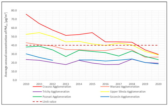
Figure 1.
Average annual concentration of PM10 [µg/m3] in selected Polish agglomerations. Source: Statistics Poland.
In parallel, the prices of residential premises in Gdańsk have been the second highest in Poland for several years (Figure 2), with the biggest growth rate compared to other cities.
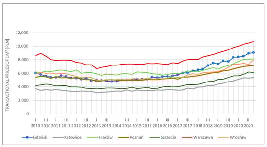
Figure 2.
Dynamics of transactional price changes in 1 m2 [PLN] on the secondary real estate market in selected Polish cities. Source: Polish National Bank.
In the Pomeranian Voivodeship, the main source of air pollution is anthropogenic emissions, of which there are three categories: surface, linear, and point sources. Surface sources are associated with industrial plants that pollute the air mainly in the fuel combustion process for energy purposes. Linear sources are associated with road, rail, water, and air transport, while surface sources are related to the municipal and residential sectors.
The main pollutant emitted from road transport in the Pomeranian zone in 2020 was nitrogen dioxides (NO2) (Figure 3). The largest share in linear emissions in the Pomeranian Voivodeship in 2020 was had by roads with the highest traffic intensity. Figure 3 presents the level of average annual concentrations of nitrogen dioxide, measured by five reference air quality monitoring stations located on five streets in Gdańsk.
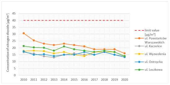
Figure 3.
Average annual concentration of nitrogen dioxide [µg/m3]. Source: ARMAG Foundation.
Compact, low-rise buildings and related heating processes in the municipal and residential sector (surface emissions) cause high concentrations, primarily of particulate matter (PM10). In the Pomeranian Voivodeship, the highest density of low-rise buildings is concentrated mainly in smaller cities and around the Gdańsk agglomeration, offering proximity to the city of Gdańsk, and at the same time, offering the peace and quiet of areas outside the city. In Gdańsk, though, the annual concentration of PM10 is below the limit value in all four reference PM10 monitoring stations (Figure 4).
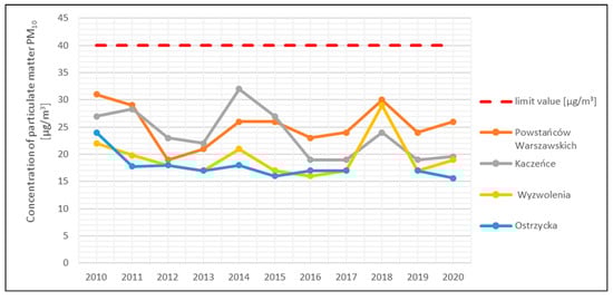
Figure 4.
Average annual concentration of particulate matter PM10 [µg/m3]. Source: ARMAG Foundation.
Compared to 2010, 2020 showed a reduction in the average annual concentration of NO2 and PM10 (Figure 3 and Figure 4), which resulted in improved air quality in the described region. Despite this positive trend, many problems require quick and more determined action. These include high emissions of pollutants from individual heating systems as well as emissions from road traffic, a small share of renewable energy sources, high noise intensity from road traffic, an increase in the number of means of transport, an increase in electromagnetic field levels, and the still low level of environmental awareness among the general population.
Prices of residential premises are primarily a function of two factors: the supply and demand relationship and production costs. Supply and demand are influenced by general social and macroeconomic phenomena. Among the key variables for housing price formation are gross domestic product (GDP), inflation, interest rate level, income levels, and unemployment rate. What is worth mentioning is that their strength and impact, even in the scale of one city, may differ from one district to another [41], which is a confirmation of the fact that residential premise prices are very much location related.
In terms of social factors influencing demand in the residential premises market, there can be mentioned migrations, demographic factors, settlement preferences, and patterns of social life. The specificity of the described real estate market sector lies in the fact that the demand fluctuates while the supply is rigid due to the limited land resources, limited number of premises in the near-term period, and regulatory reasons [42]. Furthermore, factors influencing supply and demand interact with variable intensity in given periods of time. Another characteristic of the residential premise’s market is, therefore, seasonality.
To investigate the specificity of the dynamics of real estate prices in Gdańsk in the analysed period, it is necessary to analyse the factors which determine it on the local level.
In the last decade, economic parameters were at a high level, resulting in significant development within the city. Due to the stable growth of income (Figure 5) combined with a low level of unemployment (Figure 6) and historically low interest rates, demand for residential premises grew rapidly.
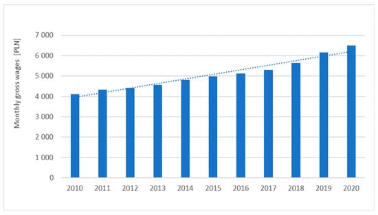
Figure 5.
Average monthly gross wages in Gdańsk [PLN]. Source: Statistics Poland.
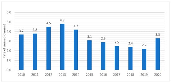
Figure 6.
Annual rate of unemployment in Gdańsk. Source: Statistics Poland.
Growing demand is reflected in the steady growth of the number of sold premises (Figure 7), which, as shown above, is characterised by significant seasonality. Residential premises in Gdańsk are purchased for private use as well as for sale or rental (capital investment).
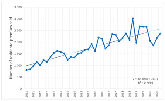
Figure 7.
Number of residential premises sold in Gdańsk (quarterly). Source: Statistics Poland.
The economic development of Gdańsk and the high quality of life resulted in the permanent inflow of population for permanent residence. Although in 2020, this was disrupted by the COVID-19 pandemic (Figure 8).
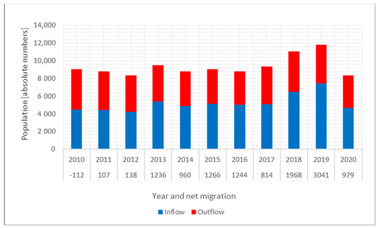
Figure 8.
Migration of population for permanent residence in Gdańsk; balance below horizontal axis. Source: Statistics Poland.
Positive net migration—understood as an inflow of population for permanent residence—is an additional factor creating demand for residential premises.
In the analysed period, growing demand was followed and supported by the growing number of dwellings completed, especially after 2014, which relates to rebounding from the after-crisis decline on an international scale in the years before (Figure 9).
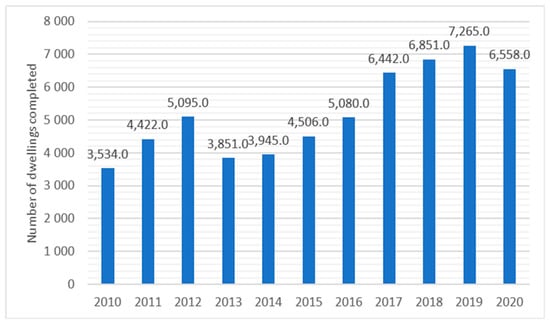
Figure 9.
Number of dwellings completed in Gdańsk. Source: Statistics Poland.
Complex relations between the supply and demand are reflected in the level and dynamics of residential premises prices, as shown below (Figure 10).
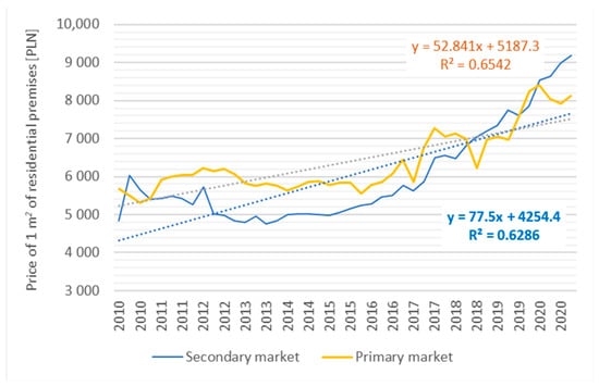
Figure 10.
Average price of 1 m2 of residential premises in Gdańsk [PLN] Source: Statistics Poland.
In the last decade, both secondary and primary markets experienced high growth, especially after 2014, when premises from the secondary market were above 83%.
The spatial policies of cities sometimes vary. In most cities, spatial planning is carried out inconsistently and sometimes based only on gaining more intensive development. There are many cities in the world that have been affected by the smog problem for a relatively long time and have been fighting it for a long time. It manifests itself in various ways, from small changes in traffic organisation or the popularisation of public transportation or bicycling to the creation of whole concepts of cities that are supposed to be smog-proof from the very beginning. Since an effective policy to reduce air pollution is a complex and long-term process, architects and urban planners have a special opportunity to creatively reexamine the city’s structure for adequate solutions inspired by the idea of sustainable development, with an emphasis on the air quality aspect.
2. Materials and Methods
2.1. Data
We analysed the air pollution in the city of Gdańsk over the period 2010–2020 using primary data received from referenced sensors.
The study considers selected data on the real estate market and selected results of pollutant concentration measurements that are crucial with respect to the discussed problem. All data is aggregated into quarterly periods by summation and averaging. It must be underlined that such a correlation between air pollution and real estate market prices was carried out for the first time in Poland. Moreover, market prices were taken from the National Statistics database as contractual prices registered by relevant district courts, not as offer prices. The second advantage of the study was the long (10 years) period of the dataset and the related high sample size.
The following data were gathered: 31 variables from the real estate market (Table 1) and air pollutant concentrations (PM2.5, PM10, NO2, and O3) (taken from the respective Regional Inspectorates of Environmental Protection). Air quality monitoring stations in Poland, operating within the State Environmental Monitoring, are located in accordance with the criteria of representativeness set out in national and European legal acts (e.g., directive 2008/50/EC of the European Parliament and of the Council of 21 May 2008 on ambient air quality and cleaner air for Europe). The provider of the data is the Agency of Regional Air Quality Monitoring in Gdansk (ARMAAG), which cooperates closely with the authors.

Table 1.
Real estate data are quarterly. The source of the data is the Central Statistical Office from the period 2010 to 2020.
The system is being successively developed. Therefore, the number of air quality monitoring stations changed slightly during the period under the presented analyses; the number of stations in which the concentrations of individual pollutants are measured varied. Overall, depending on the pollution and year, data from the following number of measuring stations were acquired in Gdańsk: NO2—9 stations, O3—3–4 stations, PM10—8–9 stations, and PM2.5—1 station.
Of the air quality monitoring stations operating in the cities, one station served as a traffic station, while the remaining ones were urban background stations. Ozone concentrations were measured only at background stations. For the purposes of the analyses, data from all measuring stations that operated in each city were used, regardless of their functions. This approach was adopted because of the relatively small number of stations in each city and the consequent inability to accurately assign specific fractions of the city’s population to each measuring station. This is so, especially because not all stations measure all types of pollutants, and in some cases, only one station in the whole city measures the concentration of pollutants (e.g., PM2.5 in Gdańsk).
To build models, quarterly data from a particular area were used. If necessary, daily means or sums were calculated, depending on the data characteristics, to reflect day-to-day variability.
2.2. Methods
To achieve the goal, this study uses the highest quality data about transaction prices and the number of residential units sold: from the most reliable real estate market data source in Poland, Statistics Poland (GUS). On the side of air pollution factors, the highest possible quality of measurement data is also provided: results of air pollution measurements from reference stations of our automatic air quality monitoring network. These two elements ensure the reliability of conclusions obtained from stochastic cause-and-effect models. The selected models for the identification of real estate market factors associated with selected air pollution parameters are the best and most effective, in the opinion of the authors of this paper as well as in the opinion of the authors of other studies. The models allow the precise identification of the influence of factors at any measurement scale, both in terms of interacting factors alone and the combined influence of a sequence of these factors together with their interactions.
At present, there are no models more effective at capturing both factors and their interactions in such a broad spectrum on the causal side of the models. Ensuring the highest quality data at this methodological stage and clarifying the model linkages is expected to give reliable conclusions on the effects side.
All findings presented in this paper will provide a comparative background for the other agglomerations (Warsaw, Cracow) covered by this study in the context of varying degrees of air pollution in Poland. At the next stage of this study, each agglomeration will be analysed more deeply, including a breakdown into neighbourhoods, to identify more precisely the impact of air pollution on the real estate market.
Now, it is not yet possible to build spatial models for each agglomeration, as the necessary source data do not exist, and we are at the stage of collecting source material.
The impact of air pollution on the development of transaction prices as well as on the number of housing units sold is crucial for the sustainable development of the regions under study for the following reasons, if no other:
- -
- the possibility of drawing conclusions as to the stage of social development (e.g., environmental awareness) of a given agglomeration,
- -
- verification of whether and to what extent environmental elements influence real estate purchase decisions in selected areas,
- -
- identification of the magnitude of air pollution as a factor that reduces the quality of life, especially if it concerns the place of residence.
All input air pollutants concentrations data were collected as 1-h mean values. For the analyses, i.e., identification of factors and interactions, they were transformed to quarterly averages. Data were subjected to a detailed quality analysis (1-h data) involving, if possible, a stage of interpolation of missing data as well as a detailed, multi-stage analysis of the causes of irregularities based on robust estimators (DFITS, Cook’s distance, Mahalanobis distance, and classic Grubb’s and Rosner’s tests). The scope of the description of the applied diagnostic methods of measurement data is enormous. Missing data were either interpolated with appropriate methods or removed by cases or variables.
The study used the Eco Data Miner analytical system developed by the authors, in which various proprietary methods and models for missing data interpolation are embedded. The variables representing the results of 1-h measurements of air pollutant concentrations for the years 2010–2020 were subjected to interpolation. The next data, after interpolation, were averaged to quarters. This procedure ensures the high quality of the measurement data. The real estate market variables had no shortcomings.
The interpolation methods depended on the length of the series of missing data (Table 2), the pollutant concentration type and the measuring station’s spatial location. The procedure is as follows: in the series of results of one-hour measurements of pollutant concentrations from reference stations, the series of data gaps were selected. As a result of the analysis of the series of missing data, all series of missing observations and estimated information resources before and after the occurrence of the series were identified to select the method/model of interpolation as described in Table 3. The series of deficiencies in the data was the basis for the construction of the distributions of missing data so that, on this basis, the appropriate interpolation method and model could be chosen.
Table 2.
Methods of interpolation of missing data depending on the length of the series of missing data.
Table 3.
Interpolation methods used.
Synthetic characteristics of the interpolation methods used in this study:
- -
- general average—the average as a consistent, unbiased and effective estimator is suitable for interpolation for reporting purposes; it was not used for forecasting models in the time domain and in GRM models, especially short-term ones, because stabilizing the short-term process at the long-term reference level leads directly to errors;
- -
- neighbour mean—unweighted mean calculated from the declared number of observations before and after; automatically, by means of an algorithm; the correctness of the available information is checked and verified before starting the interpolation;
- -
- weighted average of adjacent—weighted average calculated from the declared number of observations before and after; implemented system of weights (symmetrically into the past and future, starting from the nearest in time): 100, 30, 10, further 5; weights are standardized (zi = (xi − x0)/S) before starting interpolation;
- -
- general median—the median as a robust estimator is suitable for interpolation for reporting in high volatility situations; it should not be used, such as the average, for time-domain forecasting models, especially short-term ones;
- -
- adjacent weighted median—unweighted median calculated from the declared number of observations before and after; weighted median calculated from the declared number of observations before and after; implemented system of weights (symmetrically into the past and future, starting from the nearest in time): 100, 30, 10, further 5; weights are standardized (zi = (xi − x0)/S) before starting interpolation;
- -
- spatial weighted average (s; t)—weighted average calculated from the declared number of observations before and after; the algorithm automatically checks and verifies the correctness of the available information before starting the interpolation; system of weights (symmetrically into the past and the future, starting from the nearest in time): 100, 30, 10, further 5; weights are standardized before interpolation begins.
Before executing this method, the nature of the selected variables should be determined: dependent (variable to be interpolated), independent (variables used as input from spatial interpolation), and final (interpolated) values are computed as time-weighted means corrected with spatial average values of independent variables. This method was most often used in practice.
Aggregation to quarterly data and data collection over a period of ten years determines the time horizon of conclusions. The models are long-term. All regularities identified by the models should be considered long-term. Aggregation to quarterly data allows conclusions to be drawn in a shorter period, e.g., split up into seasons. As such, the impact of air pollutants is considered short-term. Contrary to classical time series models, the models used in this study cannot be treated as short-term models in terms of time series because they require hourly aggregated data. This allows the identification of regularities in the daily cycle (24 h), which is key for photochemical changes in air pollutants concentrations. Neither the data nor the models used in the study enable estimation in a very short period, i.e., the daily cycle. Conclusions resulting from this study should be considered long-term, allowing the identification of regularities in shorter periods of time outside the daily cycle.
Models and short-term conclusions relate to quarterly data. The models and data used in the study are based on a ten-year time horizon and are quarterly aggregated. In this study, the concept of short-term conclusions refers to a period no longer than a season. Neither the data nor the models enable the identification of regularities in the shortest cycle, i.e., the daily one.
To determine and characterise the statistically significant effects of single variables along with their interactions on the investigated real estate outcomes, we identified statistical models belonging to the family of GRM (general regression models). It must be underlined that the implementation of the GRM model to the correlation between the given phenomena was carried out for the very first time.
GRM models use the concept of the general linear model (GLM), enabling the capture of the nonlinearity of the impact of cause-and-effect relationships at the stage of link function as well as through the interactions of independent factors. GRM models represented both air pollution and the real estate market. The identification of interactions is a particularly important element of the presented research. The GRM models and identification process are given a detailed description in previous works [43,44].
Identification of the effects upon the real estate of exposure to airborne pollutants was based on the constructed GRM. It enables studying complex experimental systems and can include both qualitative and quantitative variables. This is particularly important when analysing data expressed in different measurement scales. An important advantage is also the ability to describe curvilinear relationships between variables. It is possible to use appropriate transformations of the predictors as well as the application of substitution methods using a standardised variable and a series of selected transformations of linearising variables and through a nonlinear linking function. Models were transformed into linear ones to show the most important relationships.
Data preprocessing and calculations were performed in Statistica version 13 (TIBCO Software Inc., Palo Alto, USA) and dedicated EDM Eco Data Miner version 1.09.
3. Results
The process of identifying the GRM cause and effect models of the impact of air pollutants on the parameters of the real estate market was carried out in three stages (Figure 11).
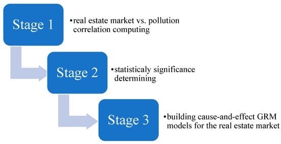
Figure 11.
Results computing flowchart.
Stage 1—calculates the correlation between the various parameters of the real estate market and pollution (expressed as total Pearson correlations). Statistically significant correlations (p ≤ 0.05) made it possible to determine which pollutants affect which parameters of the real estate market, broken down by segments (Table 4).
Table 4.
Total correlations of real estate market parameters with pollutant concentrations broken down into segments p ≤ 0.05.
The obtained results (Table 4) indicate that PM2.5 concentrations are related (p ≤ 0.05) to the number of sales of large flats above 80 m2 on the secondary market (PremSec80 = −0.45) and PM10 with prices for 1 m2 of small flats, i.e., up to 40 m2 in the secondary market (Price1mSec40 = 0.31).
The higher the concentration of pollutants, the lower the number of sales of large premises larger than 80 m2 in the area (Figure 12).
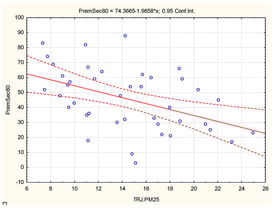
Figure 12.
The regression model of the impact of PM2.5 concentrations in Gdańsk on the sale of apartments larger than 80 m2 in area on the secondary market.
The higher the concentration of pollutants, the lower the number of sales of residential premises with 80 m2 and above area. In areas with high pollution concentration (i.e., the city centre), the percentage of large dwellings (and hence the number of transactions with them) is lower than in areas with low pollution concentration.
The average transaction prices of 1 m2 of small flats below 40 m2 are the highest in the areas with the highest concentration of air pollutants, which is related to the fact that the highest average prices per 1 m2 are in the city centre, where small flats predominate, and the concentration of air pollutants is high.
This stage allowed for the identification of PM2.5 and PM10 dust pollution as potential factors related to both the number of offers and the prices of real estate on the secondary market (Figure 13).
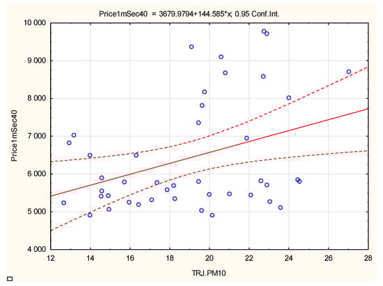
Figure 13.
The regression model of the impact of PM10 concentrations in Gdańsk on the selling price of flats below 40 m2 in the secondary market.
The average transaction prices of 1 m2 of small flats with less than 40 m2 (Figure 13) are the highest in the areas with the highest concentration of air pollutants, which is related to the fact that the highest average price per 1 m2 is in the city centre, where small flats dominate, and the concentration of air pollutants is high.
This stage allowed for the identification of NO2 and PM10 dust pollution as potential factors related to both the number of offers and the prices of real estate on the secondary market.
In stage 2, the direction of causality in the models was reversed, and the question was which real estate parameters were statistically significantly associated with PM10, PM2.5, NO2, and O3? The dependent variables in models were pollutants, and endogenous variables were taken from selected real estate parameters (Table 5).
Table 5.
Summary of estimations results of the hypothetical effect of real estate market parameters on pollutant concentrations, p ≤ 0.05.
GRM models with interactions were built for each relationship of the effect on concentrations. On this basis, additional models were identified in relation to the stage of total correlation analysis. They showed significant relationships between concentrations and real estate market parameters (Table 5).
Based on the results of stage 1 and stage 2, i.e., for each real estate market parameter (dependent variables), detailed cause-and-effect GRM models (Table 6) of the relationship of the impact of pollutants on the parameters of the real estate market were built, which at the significance level of 0.05 indicated significant relationships between the pollutants and individual parameters with real estate market PremSec80 (Table 7).
Table 6.
Example of the results of the estimation of the model of the influence of environmental factors on the number of sales of premises above 80 m2; secondary market; model fit measures; OLS model PremSec80.
Table 7.
Results of the estimation of the model of the influence of environmental factors on the number of sales of premises 60–80 m2; secondary market; model fit measures; separately in seasons; OLS and GRM model Price1mSec40.
Figure 14 shows the effect of the interaction of O3 (ozone) and PM2.5 on the number of transactions on the secondary market of flats with an area of 60–80 m2. Simultaneous with the decrease in the concentrations of O3 and PM2.5 is an increase in the number of sales of apartments with an area of 60–80 m2 on the secondary market in Gdańsk (Table 8).
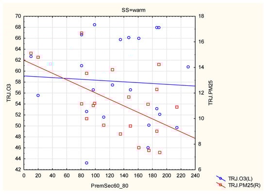
Figure 14.
The regression model of the impact of PM2.5 and O3 interaction concentrations in Gdańsk on the sale of apartments 60–80 m2 on the secondary market; warm seasons 2010–2020.
Table 8.
Results of the estimation of the model of the influence of environmental factors on the 1 m2 price of 40 m2; secondary market; model fit measures; separately in seasons; OLS and GRM model.
Figure 15 shows the interaction of the influence of PM10 and NO2 on the price of 1 m2 of residential premises with an area of 40 m2 on the secondary market in Gdańsk.
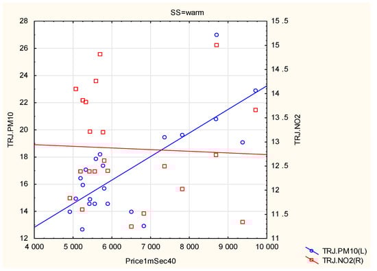
Figure 15.
Regression model of the impact of the interaction of PM10 and NO2 concentrations in Gdańsk on the selling price of flats smaller than 40 m2 in area in the secondary market; warm seasons 2010–2020.
Simultaneous with a decrease in PM10 concentrations and an increase in NO2 concentrations due to increased traffic is an increase in the price of 1 m2 of residential premises with an area of 40 m2 on the secondary market in Gdańsk.
4. Discussion
In a developed sustainable economy, the real estate market, a partly economic and partly social phenomenon, is strongly linked to the environmental element. People who are aware of the dangers of air pollution choose clean areas for living to avoid in the long term, inter alia, the health complications to which they expose themselves in heavily polluted regions. Since more than 60% of the population is living in cities, the critical question of whether the concept of sustainability is present in the selected agglomerations is still to be answered.
One reported trial was carried out in Warsaw, the capital city of Poland, in 2018. Trojanek et al. analysed the impact of proximity to urban green areas on apartment prices in Warsaw by using the hedonic method in ordinary least squares (OLS), weighted least squares (WLS), and median quantile regression (Median QR) models. Substantial evidence that proximity to an urban green area is positively linked with apartment prices was found. On average, the presence of a green area within 100 m of an apartment increases the price of a dwelling by 2.8% to 3.1%. The effect of park/forest proximity on house prices is more significant for newer apartments than those built before 1989. Were found that proximity to a park or a forest is particularly important (and has a higher implicit price as a result) in the case of buildings constructed after 1989. The impact of urban green was particularly high in the case of a post-transformation housing estate. Close vicinity (less than 100 m distance) to an urban green increased the sales prices of apartments in new residential buildings by 8.0–8.6%, depending on the model [45].
As a result of research on the real estate market in Gdańsk in 2010–2020, air pollution factors were identified that affect this market in terms of the number of sales transactions and the transaction price. In the analysis of correlations, the statistical GRM model and the OLS regression model were used. They indicated the concentrations of PM10 and PM2.5 (independent variables) as the most frequently statistically significant (p ≤ 0.05) related to the variables representing the real estate market (dependent variables) in the price indices of a square meter of a flat.
In addition to statistically significant relationships, the apparentness of the identified relationships and their real nature should be considered. The notion of apparent relationships should not be understood as direct relationships of cause and effect but relationships in which air pollution affects the phenomenon in a general sense.
The secondary effect produces statistically significant relationships. An example is the centres of urban and industrial agglomerations, where housing prices are very high, which is associated with increased sales of small premises.
The fact of high concentrations of air pollutants in these areas is naturally associated with high prices.
In the case of large premises, i.e., those over 80 m2, the relationship between the number of sales and PM2.5 concentrations seems real and rational: an increase in concentrations causes a decrease in sales. City residents, since they choose large premises, choose cleaner areas outside the city centre (Table 9).
Table 9.
Environmental factors influencing the parameters of the real estate market, p ≤ 0.05; years 2010 to 2020.
However, some issues related to the study should be specified. The first issue concerns the number and location of reference sensors, which allowed us to develop the models and conclude general statements for the city of Gdańsk and its real estate market. Although considering the city’s spatial, economic, and social diversity, an interesting step deeper into the study would be to differentiate results and to determine the correlation level by specific districts. This, however, would require a substantive development of the sensor network in the city.
Another issue may have its source in the specificity of Gdańsk’s location—on the shore of the sea, with the direct climatic impact of the sea. Therefore, it is a future challenge to extend the research to other cities with different location and a different spatial specificity. Similar studies have already been performed [43].
It would also be worth implementing the aspect of population density. Since some districts or even streets are more heavily populated (for various reasons, such as historical settlements, post-war urbanization, etc.), it may have an impact on real estate prices. Moreover, the transport infrastructure or other urban infrastructure in the vicinity might be an additional factor affecting the searched correlation. This, however, would extend the model to the multi-dimensional problem.
Finally, the study shows the statistical correlation between the given indicators (environmental and economic). However, the social aspect is another issue that could be developed in the next research towards the implementation of human preferences surveys on the impact of air pollution on the purchase of a given piece of real estate (house, flat). In addition, the received correlation might be influenced by social affluence and strongly connected with environmental awareness. At the same time, where it is of poor quality, it becomes an important factor in the property market.
5. Conclusions
With all its complexity, the real estate market is an important element of the concept of the sustainable development of countries, regions, and cities. By considering the property market comprehensively as an interaction of economic, social, technical, legislative, spatial, and environmental, as well as other factors, the assumptions of the concept of sustainable development should be strengthened in this area. The goal of sustainable and balanced development can be considered as an increase in prosperity, seen through the prism of not only the consumption of goods but also of the ecological living conditions. The objective of sustainable growth is not so much understood as an increase in the level but as an increase in the quality of life [46].
In addition to its primary function of providing for the subsistence needs of society, today’s housing market also responds to higher-level needs (especially in developed societies) that affect the quality of life. These include transport infrastructure, opportunities for human capital development (education, health care, and cultural facilities), recreational areas, neighbourhood relations, and security. In addition, in social terms, sustainable development in the housing market also aims to prevent social exclusion caused by poverty or homelessness.
Living conditions have a key impact on the quality of life and concern both the real estate itself (size, materials used, insulation against cold and dampness, energy efficiency, and finishes) and its surroundings (clean air and green areas).
In this study, GRM (general regression model) is applied to the real estate market in Gdańsk to determine and characterise the relationship between air pollution and certain parameters of this market.
Results of this research show that the average price of 1 m2 of residential premises sold in total and the number of residential premises sold in total are not sensitive to air pollution parameters.
This confirms the assumption that the air quality in Gdańsk is very high. Therefore the level of air pollutants does not significantly influence the market parameters in general. In-depth analyses which were conducted indicated three statistically significant relationships, and these are as follows: between the number of apartments sold with an area of 80 m2 or more on the secondary market and the concentration of PM2,5; between the number of apartments sold with an area of 60–80 m2 on the secondary market and the concentration of O3 and PM2,5 in interactions and only in the warm season; and between the average price of 1 m2 of a residence with an area up to 40 m2 on the secondary market and the concentration of PM10 and O3 in interactions and only in the warm season.
The study’s practical implications can be defined for the customers as one new additional factor affecting decision-making to increase awareness of the real estate price sources (i.e., the reasons for them). Moreover, both sides of the contract must place increasing weight on the quality of the air.
However, all observed correlations regard two sectors only—price dependency for properties up to 40 m2 and the number of contracts for properties above 80 m2.
There is a clear need for further study of specific cities and/or regions to define the given correlation factors that directly affect the local/regional real estate market.
However, this study has certain limitations. For example, the results of the spatial regression model might show relationships between air pollutants and residential premises prices in wealthy city districts.
Author Contributions
Conceptualization, P.O.C. and A.R.; methodology, P.O.C. and A.R.; software, P.O.C.; validation, P.O.C.; formal analysis, A.R. and M.W.; investigation, A.R. and P.O.C.; resources, A.R.; data curation, P.O.C. and A.R.; writing—original draft preparation, A.R., A.O.-J. and M.W.; writing—review and editing, E.C. and A.O.-J.; visualization, P.O.C. and A.R.; supervision, E.C.; project administration, E.C.; funding acquisition, E.C. All authors have read and agreed to the published version of the manuscript.
Funding
This research received no external funding.
Institutional Review Board Statement
Not applicable.
Informed Consent Statement
Not applicable.
Data Availability Statement
Data available on request due to restrictions e.g., privacy or ethical. The data presented in this study are available on request from the corresponding author. The data are not publicly available due to commercial character.
Conflicts of Interest
The authors declare no conflict of interest.
References
- Mazurek, H.; Badyda, A. Smog. Konsekwencje Zdrowotne Zanieczyszczeń Powietrza; Państwowy Zakład Wydawnictw Lekarskich: Warszawa, Poland, 2018. [Google Scholar]
- Jędrak, J.; Konduracka, E.; Badyda, A.; Dąbrowiecki, P. Wpływ Zanieczyszczeń Powietrza na Zdrowie; Krakowski Alarm Smogowy: Krakow, Poland, 2017. [Google Scholar]
- Szyszkowicz, M. Air Pollution and Emergency Department Visits for Suicide Attempts in Vancouver, Canada. Environ. Health Insights 2010, 4, S5662. [Google Scholar] [CrossRef] [PubMed]
- Szyszkowicz, M. Air Pollution and Emergency Department Visits for Depression in Edmonton, Canada. Int. J. Occup. Med. Environ. Health 2007, 20, 241. [Google Scholar] [CrossRef] [PubMed]
- Weir, K. Smog in Our Brains, American Psychological Association. Available online: https://www.apa.org/monitor/2012/07-08/smog/ (accessed on 11 May 2020).
- Air Pollution and Dementia, Alzheimer’s Society. Available online: https://www.alzheimers.org.uk/about-dementia/risk-factors-and-prevention/air-pollution-and-dementia/ (accessed on 13 May 2020).
- Zhang, X.; Chen, X.; Zhang, X. The impact of exposure to air pollution on cognitive performance. Proc. Natl. Acad. Sci. USA 2018, 115, 9193–9197. [Google Scholar] [CrossRef] [PubMed]
- Bereitschaft, B.; Debbage, K. Urban Form, Air Pollution, and CO 2 Emissions in Large U.S. Metropolitan Areas. Prof. Geogr. 2013, 65, 612–635. [Google Scholar] [CrossRef]
- McCarty, J.; Kaza, N. Urban Form and Air Quality in the United States. Landsc. Urban Plan. 2015, 139, 168–179. [Google Scholar] [CrossRef]
- Cárdenas, R.M.; Dupont-Courtade, L.; Oueslati, W. Air Pollution and Urban Structure Linkages: Evidence from European Cities. Renew. Sustain. Energy Rev. 2016, 53, 1–9. [Google Scholar] [CrossRef]
- Stone, B. Urban Sprawl and Air Quality in Large US Cities. J. Environ. Manag. 2008, 86, 688–698. [Google Scholar] [CrossRef]
- Clark, L.P.; Millet, D.B.; Marshall, J.D. Air Quality and Urban Form in U.S. Urban Areas: Evidence from Regulatory Monitors. Environ. Sci. Technol. 2011, 45, 7028–7035. [Google Scholar] [CrossRef]
- Wang, Z.; Fang, C. Spatial-temporal characteristics and determinants of PM2.5 in the Bohai Rim urban area. Chemosphere 2016, 148, 148–162. [Google Scholar] [CrossRef]
- Sun, C.; Chen, X.; Zhang, S.; Li, T. Can changes in urban form affect PM2.5 concentration? Comparative analysis from 286 prefecture-level cities in China. Sustainability 2021, 13, 2187. [Google Scholar] [CrossRef]
- Bechle, M.J.; Millet, D.B.; Marshall, J.D. Effects of Income and Urban Form on Urban NO 2 : Global Evidence from Satellites. Environ. Sci. Technol. 2011, 45, 4914–4919. [Google Scholar] [CrossRef] [PubMed]
- Czechowski, P.; Piksa, K.; Dąbrowiecki, P.; Oniszczuk Jastrząbek, A.; Czermański, E.; Owczarek, T.; Badyda, A.; Cirella, G.T. Financing costs and health effects of air pollution in the Tri-City agglomeration. J. Front. Public Health Spec. Sect. Health Econ. 2022, 10, 831312. [Google Scholar] [CrossRef] [PubMed]
- Czechowski, P.O.; Dąbrowiecki, P.; Oniszczuk-Jastrząbek, A.; Bielawska, M.; Czermański, E.; Owczarek, T.; Rogula-Kopiec, P.; Badyda, A. A preliminary attempt at the identification and financial estimation of the ngative health effects of urban and industrial air pollution based on the agglomeration of Gdańsk. Sustainability 2020, 12, 42. [Google Scholar] [CrossRef]
- Kruk, H. Konkurencyjność przedsiębiorstw w świetle zasad rozwoju zrównoważonego. In Przedsiębiorstwo w otoczeniu globalnym; Dębicka, O., Oniszczuk-Jastrząbek, A., Gutowski, T., Winiarski, J., Eds.; UG: Gdańsk, Poland, 2009; Volume 116. [Google Scholar]
- Oniszczuk-Jastrząbek, A.; Dębicka, O. Economic Dimension of the Concept of Company’s Sustainable Development. In The Selected Problems for the Development Support of Management Knowledge Base; Hittmár, Š., Ed.; University of Zilina: Zilina, Czech Republic, 2014; pp. 222–225. [Google Scholar]
- Kryk, B. Wycena Strat Ekologicznych Wynikających z Działalności Energetyki w Regionie Szczecińskim. Ph.D. Thesis, Wydział Ekonomiczny US, Szczecin, Poland, 1993. [Google Scholar]
- Kryk, B. Ekorozwój jako przyjęta koncepcja rozwoju społeczno-ekonomicznego a inwestycje ekologiczne. Zesz. Nauk. Uniw. Szczecińskiego Pr. Katedr. Mikroekon. Probl. Mikroekonom. Menedżerskiej 2003, 8, 367. [Google Scholar]
- Impact Assessment. Accompanying Document to the White Paper; SEC (2011) 358 Final; European Commission: Brussels, Belgium, 2011.
- Ridker, R.G.; Henning, J.A. The determinants of residential property values with special reference to air pollution. Rev. Econ. Stat. 1967, 49, 246–257. [Google Scholar] [CrossRef]
- Huang, Z.; Du, X. Does air pollution affect investor cognition and land valuation? Evidence from the Chinese land market. J. Am. Real Estate Urban Econ. Assoc. 2022, 50, 593–613. [Google Scholar] [CrossRef]
- Boyle, M.A.; Kiel, K.A. A survey of house price hedonic studies of the impact of environmental externalities. J. Real Estate Lit. 2001, 9, 117–144. [Google Scholar] [CrossRef]
- Deyak, T.A.; Smith, V.K. Residential property values and air pollution-some new evidence. Q. Rev. Econ. Bus. 1974, 14, 93–100. [Google Scholar]
- Harrison Jr, D.; Rubinfeld, D.L. Hedonic housing prices and the demand for clean air. J. Environ. Econ. Manag. 1978, 5, 81–102. [Google Scholar] [CrossRef]
- Murdoch, J.C.; Thayer, M.A. Hedonic price estimation of variable urban air quality. J. Environ. Econ. Manag. 1988, 15, 143–146. [Google Scholar] [CrossRef]
- Wieand, K.F. Air pollution and property values: A study of the St. louis area. J. Reg. Sci. 1973, 13, 91–95. [Google Scholar] [CrossRef]
- Li, M.M.; Brown, H.J. Micro-neighborhood externalities and hedonic housing prices. Land Econ. 1980, 56, 125–141. [Google Scholar] [CrossRef]
- Ekeland, I.; Heckman, J.J.; Nesheim, L. Identifying Hedonic Models. Am. Econ. Rev. 2002, 92, 304–309. [Google Scholar] [CrossRef]
- Raya, J.M.; Estévez, P.G.; Prado-Román, C.; Pruñonosa, J.T. Living in a Smart City Affects the Value of a Dwelling? In W BT-Sustainable Smart Cities: Creating Spaces for Technological, Social and Business Development; Peris-Ortiz, M., Bennett, D.R., Pérez Bustamante Yábar, D., Eds.; Springer International Publishing: Cham, Switzerland, 2017. [Google Scholar]
- Ligus, M.; Peternek, P. Impacts of Urban Environmental Attributes on Residential Housing Prices in Warsaw (Poland): Spatial Hedonic Analysis of City Districts. In BT-Contemporary Trends and Challenges in Finance; Jajuga, K., Orlowski, L.T., Staehr, K., Eds.; Springer International Publishing: Cham, Switzerland, 2017. [Google Scholar]
- Kim, S.G.; Yoon, S. Measuring the value of airborne particulate matter reduction in Seoul. Air Qual. Atmos. Health 2019, 12, 549–560. [Google Scholar] [CrossRef]
- Izón, G.M.; Hand, M.S.; Mccollum, D.W.; Thacher, J.A.; Berrens, R.P. Proximity to Natural Amenities: A Seemingly Unrelated Hedonic Regression Model with Spatial Durbin and Spatial Error Processes. Grow. Chang. 2016, 47, 461–480. [Google Scholar] [CrossRef]
- De, U.K.; Vupru, V. Location and neighbourhood conditions for housing choice and its rental value: Empiryczne badanie w miejskim obszarze północno-wschodnich Indii. Int. J. Hous. Markets Anal. 2017, 10, 519–538. [Google Scholar] [CrossRef]
- Zhang, H.Y.; Wang, X.Y. Effectiveness of Macro-regulation Policies on Housing Prices: A Spatial Quantile Regression Approach. Hous. Theor. Soc. 2016, 33, 23–40. [Google Scholar] [CrossRef]
- Qashou, Y.; Samour, A.; Abumunshar, M. Does the Real Estate Market and Renewable Energy Induce Carbon Dioxide Emissions? Novel Evidence from Turkey. Energies 2022, 15, 763. [Google Scholar] [CrossRef]
- Ma, P.; Tao, F.; Gao, L.; Leng, S.; Yang, K.; Zhou, T. Retrieval of Fine-Grained PM2.5 Spatiotemporal Resolution Based on Multiple Machine Learning Models. Remote Sens. 2022, 14, 599. [Google Scholar] [CrossRef]
- Nykiel, L. Rynek Mieszkaniowy w Polsce; Zeszyt Hipoteczny nr 25; Fundacja na Rzecz Kredytu Hipotecznego: Warszawa, Poland, 2008. [Google Scholar]
- Łaszek, J. Bariery Rozwoju Rynku Nieruchomości Mieszkaniowych w Polsce; Materiały i studia, No 184; Narodowy Bank Polski: Warszawa, Poland, 2004; Volume 12. [Google Scholar]
- Dąbrowiecki, P.; Badyda, A.; Chciałowski, A.; Czechowski, P.O.; Wrotek, A. Influence of selected air pollutants on mortality and pneumonia burden in three Polish cities over the years 2011–2018. J. Clin. Med. 2022, 11, 3084. [Google Scholar] [CrossRef]
- Liu, R.; Yu, C.; Liu, C.; Jiang, J.; Xu, J. Impacts of Haze on Housing Prices: An Empirical Analysis Based on Data from Chengdu (China). Int. J. Environ. Res. Public Health 2018, 15, 1161. [Google Scholar] [CrossRef] [PubMed]
- Wrotek, A.; Badyda, A.; Czechowski, P.O.; Jackowska, T. Air Pollutants’ Concentrations Are Associated with Increased Number of RSV Hospitalizations in Polish Children. J. Clin. Med. 2021, 10, 3224. [Google Scholar] [CrossRef] [PubMed]
- Trojanek, R.; Głuszak, M.; Tanas, J. The effect of urban green spaces on house prices in Warsaw. Int. J. Strateg. Prop. Manag. 2018, 22, 358–371. [Google Scholar] [CrossRef]
- Pakulska, T.; Poniatowska-Jaksch, M. Rozwój Zrównoważony—“Szeroka i Wąska” Interpretaccja, Stan Wiedzy. Available online: www.sgh.waw.pl/katedry/kge/BADANIA_NAUKOWE/rozwoj%20zrownowazony-strona%20www_1.pdf (accessed on 30 October 2022).
Disclaimer/Publisher’s Note: The statements, opinions and data contained in all publications are solely those of the individual author(s) and contributor(s) and not of MDPI and/or the editor(s). MDPI and/or the editor(s) disclaim responsibility for any injury to people or property resulting from any ideas, methods, instructions or products referred to in the content. |
© 2023 by the authors. Licensee MDPI, Basel, Switzerland. This article is an open access article distributed under the terms and conditions of the Creative Commons Attribution (CC BY) license (https://creativecommons.org/licenses/by/4.0/).