Abstract
In order to improve the level of new energy consumption and reduce the dependence of the power system on traditional fossil energy, this paper proposed a bi-level optimization model for virtual power plant member selection by means of coordination and complementarity among different power sources, aiming at optimizing system economy and clean energy consumption capacity and combining it with the time sequence of load power consumption. The method comprises the following steps: (1) The processing load, wind power, and photovoltaic data by using ordered clustering to reflect the time sequence correlation between new energy and load and (2) uses a double-layer optimization model, wherein the upper layer calculates the capacity configuration of thermal power and energy storage units in a virtual power plant and selects the new energy units to participate in dispatching by considering the utility coefficient of the new energy units and the environmental benefit of the thermal power units. The Latin hypercube sampling (LHS) method was used to generate a large number of subsequences and the mixed integer linear programming (MILP) algorithm was used to calculate the optimal operation scheme of the system. The simulation results showed that by reducing the combination of subsequences between units and establishing a reasonable unit capacity allocation model, the average daily VPP revenue increased by RMB 12,806 and the proportion of new energy generation increased by 1.8% on average, which verified the correctness of the proposed method.
1. Introduction
After 2020, China’s total terminal energy demand entered the growth stage of saturation, and the scale of supply side is in excess, and the supporting thermal power units cannot be retired immediately [1]. This makes the total installed capacity in the same area in excess, and more of the same type of power enterprises. Virtual power plants (VPP) aggregate generation side resources with different output characteristics through advanced communication, control, and network technologies to participate in power grid dispatching. Based on the software-based decentralized control structure, each entity can receive, cooperate, and respond to demand according to requirements [2,3]. VPP can take advantage of the current situation of excess resources in the generation side, give full play to the output characteristics of different members, and select the members that are more conducive to meeting the dispatching needs from the existing power plants to complete the dispatching tasks. How to judge which subsequence multiple units are in at the same time and how to select members and dispatch the units in different subsequences will test the rapid response ability of VPP.
The main objective of different VPP member combinations in existing studies is to maximize the economic benefits. Romanos P et al. proposed an operational energy management strategy that uses thermal energy storage tanks to generate electricity in conjunction with 670 MW nuclear power plants in the United Kingdom [4]. Cavazzini G et al. combined pumped storage and wind power to increase revenue and working hours [5]. In Wei C, Xu J, Liao S, et al., distributed thermostatic control load and intermittent renewable energy were combined to form VPP, which can reduce the most unbalanced power and was not affected by parameter heterogeneity, and was suitable for diversified virtual electricity [6]. Cao J, Zheng Y, Han X, et al. proposed a VPP two-stage scheduling strategy with multi-time scale optimization, which introduced external calculation to coordinate the real-time complementation of regional energy [7]. Some members can decide the unit capacity configuration and system deployment according to the demand side and power plant degradation characteristics [8,9]. Li, Z. et al. took into account the heterogeneous uncertainties from the renewable energy, market prices, and electricity loads through a risk-averse stochastic programming approach [10].
Other studies have also analyzed the characteristics of members of the VPP: Chen Y, Du Q, Wu M, et al. combined the seasonal characteristics of hydropower resources through the signing of medium-term contracts to obtain a certain flexible load reserve to minimize the daily operating cost of the VPP [11]. Sakr W S, EL-Sehiemy R A, Azmy A M, et al. considered the uncertain load demand, renewable energy, and market price of VPP, and determined the optimal capacity and location of the dispatchable load [12]. Rahimi M, Ardakani F J, and Ardakani A J established the windPDF model to speed up the uncertainty and improve the expected net profit of VPP [13]. Z. Li integrated multiple levels of renewable energy to optimize the hourly operation of distributed renewable energy generation [14]. However, the above literature did not take into account the following. (1) The seasonal variation of load in some areas is not obvious. The load curve cannot be simply replaced by the typical load of the season. (2) In the process of capacity allocation, VPP does not notice that some members also undertake the function of making up for the lack of other members while meeting the load demand, and this part of the function is not reflected, which indirectly affects the value of these members.
In order to complete the dispatching tasks of the virtual power plant to the power grid more reliably, the problem of how to design indices to select members among multiple units still needs to be solved. According to the characteristics of distributed generation such as photovoltaic and wind power generation, the index of the uncontrollable member utility coefficient was proposed, and a virtual power plant member selection model considering the time sequence of power consumption was established. First, the sample was divided into different subsequences by using ordered clustering. Then, the upper reference utility coefficient and environmental performance index were used to calculate the capacity configuration of thermal power and energy storage units in VPP and select the wind power and photovoltaic units to participate in the scheduling. The lower optimization used the MILP algorithm to calculate the optimal operation scheme of the system.
2. Data Preprocessing
The data of the load and new energy units are highly uncertain due to seasonal and climatic factors. When forecasting, it is often considered to use collection methods with less interference factors or to consider more interference factors for modeling [15,16,17]. Some clustering algorithms are also used, but the usual clustering algorithm is to disrupt the clustering samples, and then divide the samples with similar characteristics into one class. Ordered clustering seeks the optimal segmentation method without changing the order of the samples [18]. Zhao J and Liu J (2020) used ordered clustering to analyze the degradation trend of capacitors under different temperatures and humidities, and the proposed degradation fitting function could well fit the degradation trend under different stresses [19]. Ping W and Zhou H (2020) improved the K-means algorithm by using the idea of two orders to reduce the number of binning and improve the efficiency of picking equipment [20]. Gao Chun, Yu Aiqing, and Ding Yu (2021) used the recursive ordered clustering method to reduce the impact of distributed generation on the distribution network reconfiguration [21]. Yuan Tie-jiang and Cao Ji-lei (2022) used a combination of the sequential algorithm and clustering algorithm to reduce the wind power–load time sequence subsequence to improve the calculation speed of the subsequent optimal allocation process [22].
Load sample data , select different number of points p to segment, , and select the optimal segmentation position , . Divide the sample into subsequences, the sum of the squares of deviations is defined as shown in Formulas (1) and (2), and finally, the number of optimal segmentation points is determined by using the contour coefficient. The expected value of the segmented load subsequence set is used as a typical load subsequence, and the function of the contour coefficient is defined as shown in Formula (3), wherein the range of the contour coefficient is [–1, 1]. The larger the value, the better the clustering effect.
where K is the number of centroid samples; is the centroid of the centroid sample at time ; is the number of samples; is the average distance between the ith sample and all other samples in the same cluster; and is the average distance between the ith sample and all samples in the next best cluster. The number of segmentation points corresponding to the maximum contour coefficient was selected as the optimal number of segmentation points to determine the load classification scheme. The time series data of the wind power and photovoltaic units were divided into multiple subsequences in units of days according to the p segmentation points obtained by the orderly clustering of electric loads, as shown in Figure 1.
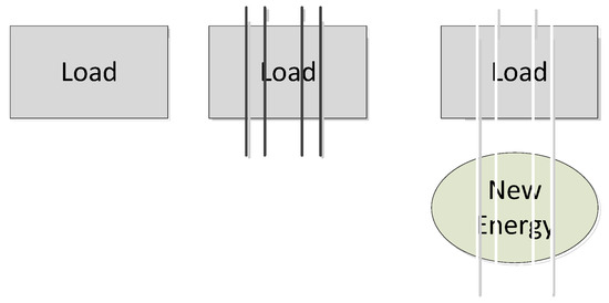
Figure 1.
Schematic diagram of new energy and load time node division based on ordered clustering.
3. Research on VPP Member Selection Architecture
3.1. System Structure of Virtual Power Plant
As is shown in Figure 2, the VPP control center exchanges information with thermal power, wind power, photovoltaic, energy storage, and general load, and arranges power output as a whole. Thermal power and energy storage, as the controllable members in the selection of VPP members, play a role in stabilizing the uncertainty of renewable energy output and ensuring the continuous and stable power supply, while wind power and photovoltaic power, as the uncontrollable members in the selection of VPP members, undertake the task of power supply together with thermal power units because of the unstable output due to weather and other factors. Load is considered to be an uncontrollable member that must be selected by the VPP because it has similar characteristics to wind and PV.
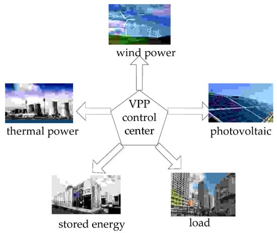
Figure 2.
Control diagram of the virtual power plant.
3.2. Bi-Level Programming Structure Design of Virtual Power Plant System
In this paper, a bi-level optimization programming method was used to optimize the member selection of the virtual power plant. The upper level is the capacity optimization module, which is used to find the optimal configuration of the system including the capacity of the controllable members and whether the uncontrollable members participate in the dispatch. This low layer is a scheduling optimization module that is used to calculate the optimal operation scheme of the system.
As shown in Figure 3, the two-level optimization contained two levels. The decision results of the upper level generally affect the objectives and constraints of the lower level, while the lower level feeds back the decision results to the upper level, thus realizing the interaction between the upper and lower levels.
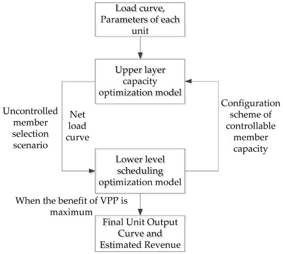
Figure 3.
Logic diagram of two-level optimization.
3.2.1. Upper Layer Capacity Optimization Model
Objective Function
The upper layer selects the utility coefficient of the uncontrollable members of the virtual power plant and the environmental performance coefficient of the controllable members as the indices for evaluating the system, which can be described as follows:
where is the utility coefficient of the uncontrollable member and is the environmental performance coefficient of the controllable member.
Utility Coefficient of Uncontrollable Member
Markowitz portfolio theory is often applied to asset allocation, which proposes that investors pursue the maximization of the expected return and the minimization of risk. VPP often faces a similar situation when choosing members, that is, VPP hopes to choose more new energy units to obtain more output, but at the same time, it has to face greater volatility risk. The risk is mainly caused by the uncertainty of the load, wind power, and photovoltaic output. In Figure 4, the solid line is the net load curve, the blue part is the adjustment interval of the net load fluctuation caused by the uncertainty of the actual output of wind power and photovoltaic power, and the dotted line is the adjustment interval of the output of controllable members adjusted by the virtual power plant. It can be seen that: ① From T1 to T2, with the increase in the net load fluctuation, the capacity of the controllable members that needs to be mobilized increases; ② in the stage from T1 to T2, when the output of the uncontrollable member is within the regulation range of the controllable member of the virtual power plant, the virtual power plant can regulate; ③ in the stage from T2 to T3, when the output of the uncontrollable member is beyond the downward regulation range of the virtual plant, the virtual power station needs to adjust the member selection to ensure the downward regulation capability; and ④ from T3 to T4, the uncontrollable members exceed the upstream regulation range of the virtual power plant, and the virtual power plant needs to adjust the member selection to ensure the upstream regulation capability.
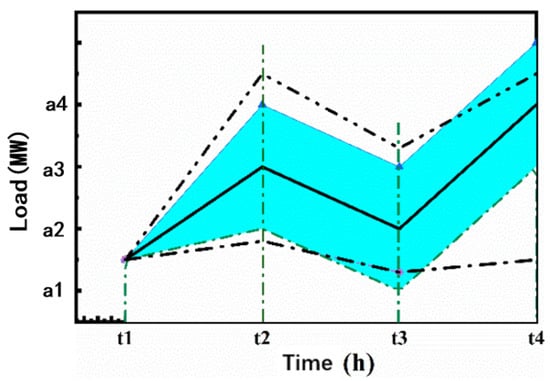
Figure 4.
Impact of the uncontrollable members on the capacity configuration of the controllable members.
Assuming that there are L uncontrollable members that can be selected by VPP, the expected expectation and variance after the combination of uncontrollable members are:
where and are the expectation and variance of the output of the ith uncontrollable member at time t under the subsequence ; is the 0–1 variable of whether the unit is selected by VPP under the subsequence ; 1 represents selection; and 0 represents elimination. is the correlation coefficient of member and is the output. and are the sum of the expectation and variance of the th generator at all times under the subsequence.
To this end, the investment utility function is used to represent the portfolio return rate:
among them, is the degree of risk aversion, which reflects the degree of the risk aversion of investors. It is generally a subjective setting variable, and the value is between [0, 4] [23]. In this paper, the value of was selected to maximize the expected total return of VPP.
Environmental Performance Indicators of Controllable Members
The flue gas discharged in the process of thermal power plant production contains harmful substances such as , , and , which pollute the surrounding environment. The emission of pollutants is directly proportional to the power generation of thermal power units:
where , , represent the emission coefficient of each pollutant, respectively, and is the total power generation of the thermal power unit under the condition of subsequence .
Controllable Member Capacity Configuration Constraint
VPP will determine the capacity of controllable members according to the output fluctuation of the selected uncontrollable members. In addition to meeting the net load demand, the thermal power will also cooperate with energy storage to increase the output to make up for the shortage of the output of uncontrollable members or reduce the output to ensure new energy consumption. When the output of the new energy unit exceeds the expected output, the thermal power unit reduces the output, in addition to meeting the output demand of the net load part, and the energy storage is used for charging when the reducing capacity is insufficient. When the output of the new energy unit fails to meet the expected output, the thermal power unit increases the output, in addition to meeting the output demand of the net load part, and the energy storage is used for supplementing the power generation for the insufficient part.
where is the actual output of the thermal power generating unit at time t of the subsequence; and are the upper and lower limits of the output of the thermal power generating unit; and and are the upper and lower limits of the climbing of thermal power generating units. is the stored energy of energy storage at time t under the condition of subsequence ; and are the upper and lower limits of the stored energy of energy storage; is the standard deviation of the net load, representing the power fluctuation of the uncontrollable member at time t of the subsequence.
Optimization Variables
The thermal power unit capacity , the energy storage capacity , and the decision variable of each uncontrollable member in the VPP member were selected as the optimization variables.
3.2.2. Lower Dispatching Optimization Model
Objective Function
The dispatching optimization model selects 24 h as the dispatching scale, takes the maximization of the VPP’s daily net revenue as the objective function, includes the net revenue of each unit, and considers the cost of the signing medium and long-term contracts between VPP and thermal power.
The net income of thermal power unit can be expressed as:
The net income of new energy units can be expressed as:
The net income of the energy storage unit can be expressed as:
The cost of VPP signing a medium- and long-term contract with thermal power can be expressed as:
where is the on-grid price of VPP, and , , and are the cost per kilowatt-hour of thermal power units, new energy units, and energy storage, respectively. , , , and are the net profits of the thermal power units, new energy units, energy storage units, and VPP under the condition of subsequence , respectively. is the cost generated by the medium- and long-term contract signed between the VPP and the thermal power unit under the condition of subsequence to ensure the energy consumption of the system. In the formula, 2 is multiplied to represent the increase and decrease of the reserve cost, respectively. is the electricity price of the medium- and long-term contract signed between the VPP and the thermal power unit. is the output of the thermal power unit at time t of the p subsequence, and is the actual output of the ith uncontrollable member excluding the load at time t under the condition of subsequence .
Constraints
- (1)
- Controllable member model
The thermal power unit scheduling constraints:
The SOC constraint of the energy storage unit is:
where and are the charge and discharge power of the energy storage at time of the subsequence, respectively; is the 0–1 variable that controls the energy storage not to be charged and discharged at the same time; and is the charge and discharge efficiency of the energy storage.
- (2)
- Uncontrollable member constraint
- (3)
- Power balance constraint
Optimization Variables
The lower layer selects the output of the thermal power unit, the charge and discharge power , of the energy storage, and the risk aversion coefficient as the optimization variables.
4. System Solution Method
4.1. Latin Hypercube Scenario Generation and Reduction
A multi-scenario approach is used to describe the uncertainty of the load and the output of the uncontrollable members. The scene generated according to ordered clustering is not as representative as a traditional typical curve such as the typical seasonal load curve, so this paper used the LHS method to generate the scene [24]. The LHS method was used to generate 1000 load scenarios and uncontrollable member output scenarios, and then the scenario reduction method considering the Kantorovich distance was used to reduce the scenarios to 10, and the two were randomly matched [25].
where is the probability of the scenario, and is the net profit of VPP in the jth scenario under the condition of subsequence .
4.2. MILP Algorithm to Solve the Lower Scheduling Optimization Problem
MILP is a kind of important mathematical programming problem that is used to solve the scheduling problem at the lower level of the model. The difference between MILP and the general programming problem is that the mathematical model of this kind of problem can be expressed by a linear relationship. A complete mathematical description of a mixed integer linear programming problem including a linear objective function for solving a maximum or minimum, a system of simultaneous linear equations, and constraints on the optimization variables is as follows:
where is the objective function; is the coefficient matrix of the simultaneous linear equations; is the value of the simultaneous linear equations; and are continuous variables and shaped variables, respectively.
5. Example Analysis
5.1. Results of Data Preprocessing
The annual load data of a region in 2021 were selected, the data time interval was 1 h, the capacity of three wind turbines was 20 MW, 30 MW, and 40 MW, respectively, and the capacity of the three photovoltaic units was 20 MW, 30 MW, and 40 MW, respectively. Formulas (1) and (2) were used to calculate the contour coefficient and find the segmentation point. The contour coefficient calculation results are shown in Table 1.

Table 1.
The contour coefficient calculation results.
As shown in Figure 5 and Table 2, the red part of the figure is the expectation of each subsequence, and the clustering results show that the differences between the subsequences are obvious and cannot simply be distinguished by seasons. The results of the contour coefficient calculation are shown in Table 3.
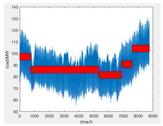
Figure 5.
Load data and ordered clustering results.
Table 2.
Load sequence segmentation.
Table 3.
Member selection scheme based on order-bilevel optimization.
5.2. Comparison of Member Selection Schemes of Two Calculation Methods
Table 3 shows the member selection scheme obtained by using the method in this paper to evaluate each member.
Table 4 shows the results of member selection by using the MILP method to maximize the total revenue of VPP after ordered clustering.
Table 4.
Member selection scheme based on the ORDING-MILP method.
Compared with the member selection of the two groups, it can be found that under the condition of sufficient consumption capacity, the bi-level optimization method proposed in this paper tended to select more clean energy unit output, which takes into account both the clean energy consumption and environmental benefits while pursuing the maximization of the VPP economic benefits. Comparing the VPP benefits of the two groups, it can be found that, except for subsequence 1, the benefits of the bi-level optimization method were higher, because this method optimized the capacity allocation of controllable members, indirectly reduced the operation and maintenance costs of thermal power and energy storage units, and increased the benefits of VPP. From the perspective of the proportion of new energy generation, comparing the two groups of subsequence 2, it can be found that when the selection scheme of uncontrollable members was the same, the proportion of new energy generation did not change significantly, which shows that the method proposed in this paper is reasonable for the capacity allocation of controllable members, and saves the operation and maintenance costs for virtual power plants while ensuring the new energy consumption capacity. Comparing subsequences 4 and 5 of the two groups, it can be found that when the uncontrollable members chose to increase one group, the method proposed in this paper could improve the overall revenue of VPP while increasing the proportion of new energy generation.
Taking subsequence 1 as an example, Figure 6 shows the 10 groups of the load subsequence generated by the LHS method, Figure 7 and Figure 8 show the output subsequence of uncontrollable members of the LHS method, and the dashed line in the figure shows the load in subsequence 1 and the output expectation of the uncontrollable members. It can be found that the peak value of the output of new energy units generally decreased between 10 o’clock and 15 o’clock. Figure 9 and Figure 10 are the output results of typical days under the two optimization methods, respectively. The red part is the thermal power output. It can be found that the output of thermal power units was smoother between 10 o’clock and 15 o’clock. This shows that the output of the uncontrollable member optimized by the bi-level optimization model proposed in this paper was smoother, which is convenient for VPP coordination.
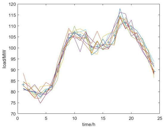
Figure 6.
LHS randomly generated load data.
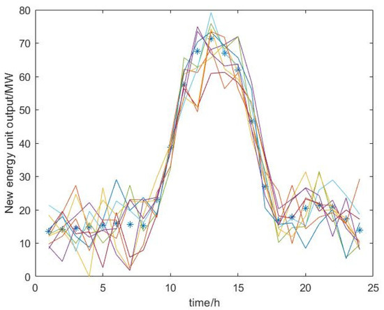
Figure 7.
The uncontrollable member effort of the order-MILP method.
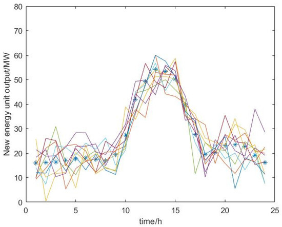
Figure 8.
Uncontrollable member effort of the order-bilevel optimization method.
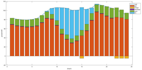
Figure 9.
Scheduling results of the order-MILP method.
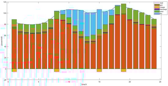
Figure 10.
Scheduling results of the order-bilevel optimization method.
6. Conclusions
With the excess power supply on the supply side, the assembled thermal power units cannot be retired immediately. By taking advantage of the output characteristics of different members of VPP, the existing power plants can choose members that can easily meet the dispatching requirements. First, the load timing was utilized to solve the problem that the load curve in some areas does not change obviously with the season. It is more reliable to divide the load curve into different subsequences by using ordered clustering. Second, the utility function of uncontrollable members was proposed to describe the risks and benefits of the uncontrollable members in VPP. It provides a basis for the capacity configuration of controllable members in VPP, reflects the value of controllable members to maintain the reliability of the VPP output, and provides a basis for the signing of medium- and long-term standby contract between the VPP and controllable members. The double-layer optimization scheme proposed by this model was compared with the method considering only the economic benefits of VPP. The average daily income of VPP was increased by RMB 12,806, and the proportion of new energy generation was increased by 1.8% on average, which verified the correctness of the proposed method. It can be found that the economic benefit, environmental benefit, and scheduling reliability are a pair of contradictory objectives. The optimization results show that there is a strong coupling relationship between the capacity of each equipment. The method proposed in this paper is suitable for the future situation of abundant data and abundant power generation resources, and provides a new idea for the VPP capacity configuration problem. It should be pointed out that this method relies on accurate prediction of the output of uncontrollable members. With the development of prediction technology, the improvement in the output prediction accuracy of new energy units is a direct optimization of this method.
Author Contributions
Y.Z. proposed the research topic, designed the model, performed the simulations, and analyzed the data. Y.W. was responsible for guidance, proposing the research topic, giving constructive suggestions, and revising the paper. X.Q. performed the simulations and analyzed the data. M.W. and X.W. improved the manuscript and corrected spelling and grammar mistakes. All authors have read and agreed to the published version of the manuscript.
Funding
This work was sponsored by the Social Science Fund Program of Jilin Province (2020B069): Research on the contribution of electricity market reform to energy consumption of enterprises in Jilin Province.
Institutional Review Board Statement
Not applicable.
Informed Consent Statement
Not applicable.
Data Availability Statement
Not applicable.
Conflicts of Interest
The authors declare no conflict of interest.
References
- Zhang, N.; Xing, L.; Lu, G. Face Prospect of China's electric power development in 2050. China Energy 2018, 3, 5–10. (In Chinese) [Google Scholar]
- Bhuiyan, E.A.; Hossain, M.Z.; Muyeen, S.M.; Fahim, S.R.; Sarker, S.K.; Das, S.K. Towards next generation virtual power plant: Technology review and frameworks. Renew. Sustain. Energy Rev. 2021, 150, 111358. [Google Scholar] [CrossRef]
- Wang, M.; Yang, M.; Fang, Z.; Wang, M.; Wu, Q. A Practical Feeder Planning Model for Urban Distribution System. IEEE Trans. Power Syst. 2022. [Google Scholar] [CrossRef]
- Romanos, P.; Al Kindi, A.A.; Pantaleo, A.M.; Markides, C.N. Flexible nuclear plants with thermal energy storage and secondary power cycles: Virtual power plant integration in a UK energy system case study. E-Prime-Adv. Electr. Eng. Electron. Energy 2022, 2, 100027. [Google Scholar]
- Cavazzini, G.; Benato, A.; Pavesi, G.; Ardizzon, G. Techno-economic benefits deriving from optimal scheduling of a Virtual Power Plant: Pumped hydro combined with wind farms. J. Energy Storage 2021, 37, 102461. [Google Scholar] [CrossRef]
- Wei, C.; Xu, J.; Liao, S.; Sun, Y.; Jiang, Y.; Ke, D.; Zhang, Z.; Wang, J. A bi-level scheduling model for virtual power plants with aggregated thermostatically controlled loads and renewable energy. Appl. Energy 2018, 224, 659–670. [Google Scholar] [CrossRef]
- Cao, J.; Zheng, Y.; Han, X.; Yang, D.; Yu, J.; Tomin, N.; Dehghanian, P. Two-stage optimization of a virtual power plant incorporating with demand response and energy complementation. Energy Rep. 2022, 8, 7374–7385. [Google Scholar] [CrossRef]
- Li, Z.; Wu, L.; Xu, Y.; Zheng, X. Stochastic-Weighted Robust Optimization Based Bi-layer Operation of A Multi-energy Home Considering Practical Thermal Loads and Battery Degradation. IEEE Trans. Sustain. Energy 2022, 13, 668–682. [Google Scholar] [CrossRef]
- Li, Z.; Xu, Y.; Feng, X.; Wu, Q. Optimal Deployment of Heterogeneous Energy Storage System in a Residential Multi-Energy Microgrid with Demand Side Management. IEEE Trans. Ind. Inform. 2020, 17, 991–1004. [Google Scholar] [CrossRef]
- Li, Z.; Wu, L.; Xu, Y.; Wang, L.; Yang, N. Distributed tri-layer risk-averse stochastic game approach for energy trading among multi-energy microgrids. Appl. Energy 2023, 331, 120282. [Google Scholar] [CrossRef]
- Chen, Y.; Du, Q.; Wu, M.; Yang, L.; Wang, H.; Lin, Z. Two-stage optimal scheduling of virtual power plant with wind-photovoltaic-hydro-storage considering flexible load reserve. Energy Rep. 2022, 8, 848–856. [Google Scholar] [CrossRef]
- Sakr, W.S.; EL-Sehiemy, R.A.; Azmy, A.M.; Abd el-Ghany, H.A. Identifying optimal border of virtual power plants considering uncertainties and demand response. Alex. Eng. J. 2022, 61, 9673–9713. [Google Scholar] [CrossRef]
- Rahimi, M.; Ardakani, F.J.; Ardakani, A.J. Optimal stochastic scheduling of electrical and thermal renewable and non-renewable resources in virtual power plant. Int. J. Electr. Power Energy Syst. 2021, 127, 106658. [Google Scholar] [CrossRef]
- Li, Z.; Xu, Y.; Fang, S.; Mazzoni, S. Optimal Placement of Heterogeneous Distributed Generators in a Grid-Connected Multi-Energy Microgrid under Uncertainties. IET Renew Power Gener. 2019, 9, 2623–2633. [Google Scholar] [CrossRef]
- Si, Z.; Yang, M.; Yu, Y.; Ding, T. Photovoltaic power forecast based on satellite images considering effects of solar position. Appl. Energy 2021, 302, 117514. [Google Scholar] [CrossRef]
- Li, P.; Yang, M.; Wu, Q. Confidence Interval Based Distributionally Robust Real-Time Economic Dispatch Approach Considering Wind Power Accommodation Risk. IEEE Trans. Sustain. Energy 2021, 12, 58–69. [Google Scholar] [CrossRef]
- Zhang, Z.; Zhao, P.; Wang, P.; Lee, W.J. Transfer Learning Featured Short-Term Combining Forecasting Model for Residential Loads With Small Sample Sets. IEEE Trans. Ind. Appl. 2022, 58, 4279–4288. [Google Scholar] [CrossRef]
- Nielsen, F.; Nock, R. Optimal interval clustering: Application to Bregman clustering and statistical mixture learning. IEEE Signal Process. Lett. 2014, 21, 1289–1292. [Google Scholar] [CrossRef]
- Zhao, J.; Liu, J. Ordered clustering method and degradation trend analysis for performance degradation of tantalum capacitor. IEEJ Trans. Electr. Electron. Eng. 2020, 15, 179–186. [Google Scholar] [CrossRef]
- Ping, W.; Zhou, H. Order Batch Optimization strategy based on improved K-means clustering algorithm. In Proceedings of the 2020 2nd International Conference on Information Technology and Computer Application (ITCA), Guangzhou, China, 18–20 December 2020; pp. 217–221. [Google Scholar]
- Gao, C.; Yu, A.Q.; Ding, Y. Multi-period dynamic reconfiguration of active distribution network based on improved recursive ordered clustering. Power Autom. Equip. 2021, 41, 84–90. (In Chinese) [Google Scholar]
- Yuan, T.J.; Cao, J.L. Optimal capacity allocation of wind-hydrogen low-carbon energy system considering wind-load uncertainty. High Volt. Technol. 2022, 48, 2037–2044. (In Chinese) [Google Scholar]
- Liu, M.; Wu, F.F. Portfolio optimization in electricity markets. Electr. Power Syst. Res. 2007, 77, 1000–1009. [Google Scholar] [CrossRef]
- Zhang, N.; Kang, C.; Kirschen, D.S.; Xia, Q.; Xi, W.; Huang, J.; Zhang, Q. Planning Pumped Storage Capacity for Wind Power Integration. IEEE Trans. Sustain. Energy 2013, 2, 393–401. [Google Scholar] [CrossRef]
- Dupačová, J.; Gröwe-Kuska, N.; Römisch, W. Scenario reduction in stochastic programming. Math. Program. 2003, 95, 493–511. [Google Scholar] [CrossRef]
Disclaimer/Publisher’s Note: The statements, opinions and data contained in all publications are solely those of the individual author(s) and contributor(s) and not of MDPI and/or the editor(s). MDPI and/or the editor(s) disclaim responsibility for any injury to people or property resulting from any ideas, methods, instructions or products referred to in the content. |
© 2023 by the authors. Licensee MDPI, Basel, Switzerland. This article is an open access article distributed under the terms and conditions of the Creative Commons Attribution (CC BY) license (https://creativecommons.org/licenses/by/4.0/).