Article

Automating Microclimate Evaluation and Optimization during Urban Design: A Rhino–Grasshopper Workflow

1
School of Architecture and Urban Planning, Hunan City University, Yiyang 413000, China
2
School of Architecture, Changsha University of Science & Technology, Changsha 410083, China
3
School of Architecture and Art, Central South University, Changsha 410083, China
*
Authors to whom correspondence should be addressed.
Sustainability 2023, 15(24), 16613; https://doi.org/10.3390/su152416613
Submission received: 20 September 2023 / Revised: 8 November 2023 / Accepted: 28 November 2023 / Published: 6 December 2023

Abstract

:
Though building-scale energy demand and indoor thermal comfort have been extensively covered by recent studies, the automation of middle- and larger-scale outdoor microclimate evaluation in parametric design is less covered. The relatively slow computation and the need for sophisticated expertise are some of the current issues. This paper proposes a Rhino–Grasshopper custom script to automatically compute spatial indicators for a quick thermal comfort estimation. The Galapagos evolutionary algorithm is used to optimize thermal comfort and select the best combinations of spatial indicators. In a summer case study located in Shantou, China, the proposed workflow was three times faster than a non-automated indicator calculation in ArcGIS, while the optimization method achieved 25% to 33% reduction in land areas under extreme heat stress. This automated process applies to existing states and new urban designs. It is adaptable to customized prediction models under different climatic zones.

1. Introduction

1.1. Background and General Context

The international rise of awareness of climate change over the last few decades has persistently proven that the current trend of global urbanization (featuring an intense energy consumption and all sorts of waste production) has many negative effects on urban ecosystems and the living environment [1]. As the growing urban population is expected to reach two-thirds of the global population in just three decades [2], international institutions are calling for changes of paradigm in the way cities are built and operated [3]. For instance, the International Panel on Climate Change (IPCC) in 2022 has once more insisted on an energy transition to net zero carbon by 2050 to keep the global temperature rise below 1.5 °C [4,5,6], one of the global aims being to promote urban sustainability measures and reduce the negative impacts of urban environments on human health and well-being [7,8,9]. Translated into urban design research and practice, this means a demand for a paradigm shift that employs new methods and tools to ensure that future urban spaces have less carbon footprints, but also that they are climate-responsive, more comfortable and healthier for urban residents.
Climate-responsive urban planning and design is an angle of urban sustainability developed over the last few decades to tackle urban heat-island effects which lead to excessive energy consumption, increased carbon emissions (atmospheric pollution), extreme heat wave incidents, etc., which are some of the most alarming consequences of “unsustainable” urban planning and design [10,11]. In the long term, climate-responsive urban planning and design combats the rise in global temperature and aims at reducing the highly related public health and mortality consequences [12,13]. Climate-responsive urban planning and design-related studies have unequivocally established that urban form, vegetation, surface materials and water bodies interact with the urban climate at the macro- and micro levels through multiple radiations and heat transfers, including direct and diffuse solar radiations on ground and wall surfaces [14,15]. These processes have been extensively studied and many analytical tools have been constructed over the past few years to predict urban physics and evaluate the microclimate in urban design projects, even at the very early stages [16,17,18,19].

1.2. State of the Art in Microclimate Evaluation

The current advances in computation technologies and the increasing accessibility of computational tools (hardware and software) are causing almost every industry to be dependent on computation tools, such as the design industry (including architectural and urban design) [20]. In recent years, computer-aided design has been adopted in all countries around the world for more efficiency in terms of design possibilities, time and cost savings, as well as the predictability at the design phase of real-life situations, one of which is the microclimate that urban spaces are subject to. This shift to computational design has also resulted into an actual shift to data-driven design and performance-driven design, which can also be understood as a shift from subjective human decision making to data-driven objective decision making [21,22,23,24].
The application of this new approach to climate-responsive urban planning and design has been possible due to several numerical simulation tools that define the state of the art in computational microclimate evaluation. Various Computational Fluid Dynamic models such as ANSYS-Fluent, PHOENICS, OpenFOAM, etc., are now allowing urban designers to simulate the wind flow in urban spaces and predict the impacts of building and landscape geometries on ventilation and heat transfers between urban surfaces [25,26,27,28]. Even more holistic models such as ENVI-met not only allow a comprehensive simulation of wind-flow and heat transfer between different urban components (geometries, materials, soil profiles, vegetations, water, etc.), but also estimate, based on human biological parameters, thermal comfort indices such as Predicted Mean Vote (PMV), Percentage People Dissatisfied (PPD), Physiological Equivalent Temperature (PET) and Universal Thermal Climate Index (UTCI) [29,30].
The recent development of parametric/algorithmic and generative designs as new methods used for architectural and urban design [31,32], characterized by a systematic and automatic exploration of countless design possibilities and, more effortlessly than ever, the generation of relevant data for urban performance analyses and decision making [33,34], is now demanding that microclimate simulation models be integrated into parametric design software environments to facilitate the responsiveness and the automatism of microclimatic analysis along with the design of urban spaces [35,36,37,38,39]. One of the prime examples of such parametric environments is the Rhino–Grasshopper environment where many third-party microclimate simulation packages such as EnergyPlus, OpenFoam, Radiance, etc., have developed into Rhino–Grasshopper 3D, and plugins such as Dragonfly, Ladybug, Honeybee, Butterfly, etc., for the purpose of integrating wind flow, solar access, heat transfers and human thermal comfort analyses into an automated and climate responsive workflow [40,41,42,43]. In consequence, Rhino–Grasshopper 3D is currently by far the tool most used by urban climate designers to automate urban microclimate evaluations along with parametric/algorithmic and generative design.
The typical application of Grasshopper plugins consists of combining their capabilities into a workflow that starts from generating multiple design scenarios parametrically, then each plugin is used to output a specific set of performance indicators which, for decision-making purposes, can be post-processed via other statistical analysis tools or optimization algorithms. For example, Shayan Mirzabeigi and Mohamad Razkenari [44], in a study intended to investigate the impact of urban typologies on building energy performance and outdoor thermal comfort, employed a Rhino–Grasshopper-based workflow that combines various Grasshopper built-in components, third-party plugins such as Dragonfly, Honeybee and Eddy3D, and custom Python scripts to set different building typologies, calculate corresponding floor area ratio (FAR) and window-to-wall ratio (WWR), process local weather data, set building thermal zones and simulate building energy use and surface temperatures. Wind speed, air temperature and relative humidity were calculated and UTCI estimated to evaluate the outdoor thermal comfort performance of multiple design scenarios. Xu et al. [45], in a study that focused on urban block design and optimization, combined Butterfly, Honeybee and Ladybug, respectively, for wind flow, solar radiation, and outdoor thermal comfort analyses. For the purpose of studying the correlations between various urban parameters and microclimates, others have exported the output data generated in Grasshopper to statistical tools such as Excel and SPSS for post processing [46]. Similar approaches have been used recently by many other microclimate evaluation-related studies [47,48,49].
Another important part of microclimate performance-driven design is the optimization of the design scheme instructed by the evaluation results. In the era of parametric/algorithmic and generative design, more and more studies and projects are integrating genetic algorithms (GAs) into their architectural and urban design workflow for the exploration and the selection of optimal schemes with specific performance objectives [50,51]. Grasshopper’s built-in optimization component Galapagos and third-party optimization plugins such as Octopus and Galapagos are some of the most used [52]. As far as climate-responsive design is concerned, many studies published over the last few years have extensively demonstrated the application of genetic optimization algorithms for microclimate performance-driven optimization of urban design. For example, in their study on urban morphology and outdoor thermal comfort, Xu et al. employed the genetic optimization algorithm Galapagos to identify the best-performing urban blocks based on the minimization of UTCI as the objective [45]. Yasser Ibrahim et al., focusing on urban courtyard blocks in hot arid zones, used the genetic optimization plugin Octopus to search for the best combinations of courtyard orientation, interspace width and building height that met UTCI and cooling load minimization targets [53]. Working on urban block typologies, Nastaran Abdollahzadeh and Nimish Biloria optimized building types, orientation, aspect ratio and window-to-wall ratio based on the minimization of UTCI and energy use [54]. Such a multi-objective optimization approach was used by many other authors to optimize different urban elements (street blocks, street patterns, street networks, building geometry, building typology, etc.) based on energy, wind and thermal comfort objectives [55,56,57,58,59].
Even though the combination of these evaluation tools (Ladybug, Honeybee, Dragonfly, Butterfly, ENVI-met, etc.) within the same parametric/algorithmic environment of Rhino–Grasshopper 3D is beneficial for an increased volume of design exploration and performance optimization, the workflow is still quite dependent upon third-party background software that limits the overall speed of the workflow. Typically for wind flow simulations, the Grasshopper plugin Butterfly is dependent upon the OpenFOAM software BlueCFD as a background program for CFD calculations. This is also the case for ENVI-met and similar plugins [60]. Air temperature and radiation calculations are run through separate EnergyPlus engines, and in some cases, additional analyses might be conducted in Excel or SPSS and the results imported back to Rhino–Grasshopper for visualization [46]. At a building scale, such operations might be relatively fast, but they require a great deal of computing power and time when it comes to urban-scale larger studies. To tackle such difficulties, a new set of approaches is being tapped into: some building a third-party toolkit such as Eddy3D [61] or a web-based interface such as City Building Energy Saver (CityBES) [62] to automate the process between multiple microclimate evaluation plugins in Grasshopper, or machine learning models trained with extensive simulation or field-measured data [63,64,65]. Eddy3D is a third-party plugin for Grasshopper, designed by Batrick Kaster and Timur Dogan to bypass the separate and time-consuming manipulations of three existing simulation engines (Radiance, EnergyPlus, and OpenFOAM) through their respective grasshopper plugins (Honeybee, Butterfly, etc.). In fact, Eddy3D is designed to handle the data preprocessing, the simulation execution and the post-processing between these three commonly used simulation engines for wind flow, mean radian temperature (MRT) and outdoor thermal comfort metric simulations [61]. CityBES is designed to simulate the energy performance of a city’s building stock; the web-based platform uses CityGML, an XML-based open data model, to represent 3D city models, and runs its energy modeling through the OpenStudio software development kit (SDK) and the EnergyPlus simulation engine [62]. Li et al. have built an artificial neural network (ANN) to predict thermal sensation votes (TSVs) based on environmental and human body parameter inputs [66]. In a study on thermal comfort in severely cold winters, Wang built an ANN model trained with CFD simulation data to predict an adapted UTCI in China with 5% error [67]. Other ANN models have been built for various purposes, including heating, ventilation and air conditioning (HVAC) system control based on thermal comfort prediction, indoor thermal comfort prediction, etc. [68,69].
Even though the prediction of microclimate via ANN has been shown to be a potential shortcut to microclimate simulation instead of computation and time-consuming CFD simulations, most of them are not integrated into an automated, parametric or generative design environment. Some recent studies have tackled this limitation by building ANN models into the Rhino–Grasshopper 3D environment. For instance, Ruinan Zhang et al. have recently built an ANN model in Rhino–Grasshopper for thermal comfort optimization in a semi-outdoor stadium. Intending to investigate the impact of the stadium’s morphology on thermal comfort (UTCI) during its use cycle, the parametric framework built in Grasshopper used the EnergyPlus and OpenFOAM simulation engines to predict thermal comfort. The evaluated average comfortable seats during the use cycle are fed into an ANN model and the Galapagos genetic algorithm is used for the optimization of three parameters (the stadium’s canopy elevation, the facade porosity and the sun-shield slant angle) [70]. Tabadkani et al., in a study on courtyard design, used input and output data obtained through Ladybug and Honeybee simulations to train a deep learning model usable for indoor thermal comfort prediction in courtyard buildings [71]. Other recent studies have adopted machine learning methods for other microclimate prediction purposes beyond the design stage (to reduce thermal comfort related energy use in buildings, improve indoor air quality, etc.) where the prediction accuracy of machine learning models can reach up to 97% [72].

1.3. Research Gap

The existing literature on urban microclimate evaluation at the design stage covers both architecture and urban design quite extensively. Under the parametric/algorithmic or generative design approach, building performance evaluation, particularly building energy demand and indoor thermal comfort, are extensively covered, but one can observe that relatively less has been achieved so far on urban design and optimization based on automated outdoor microclimate evaluation in a parametric or generative design framework. In practice, the state-of-the-art methods applicable to indoor microclimate and building energy evaluation may show some limitations in the context of parametric urban design and outdoor microclimate evaluation, primarily due to the scale difference between building design and urban design.
First, with parametric/algorithmic and generative design, the bigger scale of urban design projects requires a greater computation power for 3D model generation and numerical simulations (typically airflow and energy transfer simulations). While the state-of-the-art simulation methods that combine different simulation plugins (Butterfly, Ladybug, Honeybee, etc.) for airflow, energy transfer and thermal comfort simulations can be quite fast for building-scale projects, running similar simulations for urban-scale projects is a lot slower and require even greater computation power. In consequence, the automation of the design and its evaluation in a Rhino–Grasshopper-like parametric environment ends up being much less efficient, limiting the exploration of design scenarios and their optimization solutions.
Even though some authors have demonstrated the capabilities of a parametric design environment, such as Rhino–Grasshopper and its application to urban design and the automation of the microclimate evaluation, one can notice throughout the existing literature that most of the automation case studies have employed simplified idealistic urban models or small-scale study areas. The combination of multiple simulation engines and the application of genetic algorithms to the automatic and “real-time” optimization of middle- and large-scale urban models based on a systematic and intensive simulation of countless design scenarios would be relatively slow and inefficient.
The need for a more efficient, less computation-demanding and less time-consuming workflow for urban-scale microclimate evaluation still is quite a gap to fill in, considering the current capabilities in parametric/algorithmic design.
Besides the computation problem, the existing literature on the automation of urban-scale microclimate assessment at the design stage is mostly focused on the optimization of morphological parameters. Urban vegetation and surface materials have not been integrated in most studies on the optimization of climate-responsive urban design.
Furthermore, the automation of microclimate evaluation in urban renewal contexts has not been discussed so far. Indeed, some specific requirements on the preservation or the restricted modification of certain urban elements (buildings, roads, surface materials, etc.) represent some of the challenges and limitations to the application of genetic algorithms to urban form-finding and random design exploration during the optimization process in urban renewal contexts.

1.4. Objectives

-
Build a responsive evaluation workflow based on spatial indicators.
For an instant and responsive use at the design stage, this study attempts to develop an automated workflow for urban outdoor microclimate evaluation implemented in Rhino-Grasshopper 3D. The workflow will take in urban geometric and numerical inputs, generate the urban 3D model, extract spatial descriptive indicators from the model, assess the spatial distribution of outdoor thermal comfort and use an evolutionary optimization algorithm to generate the best combinations of spatial indicators for optimal outdoor thermal comfort. The thermal comfort output and the best combinations of spatial indicators generated by the automated program will constitute the direct feedback from the urban model. This feedback is useful for improving the design of the urban space.
-
Increase computation speed.
To increase the computation speed, the Rhino–Grasshopper script will bypass CFD simulation engines by using a custom statistical model for thermal comfort prediction based on geometric, material and vegetation indicators directly computed from the input model. Additionally, these spatial indicators are easily interpretable by designers.
-
Reduce the computation load for genetic optimization at middle- and large scale.
Because real-time 3D model generation often accounts for a large proportion of the computation power and time during the application of genetic algorithms to the design optimization, a decoupled optimization approach will be used in this study, separating the optimization of design parameters from the 3D modeling, which will improve a great deal of the overall computation efficiency and the applicability of the workflow to middle and large urban areas.
In the following sections, this paper will present the conceptual framework of this study, the automation workflow for outdoor thermal comfort assessment and optimization and the main structure of the Rhino–Grasshopper script along with its step-by-step functions. Then, a case study will be presented showing the different steps, their inputs and outputs and a performance evaluation of the Grasshopper script.

2. Methodology

2.1. Conceptual Framework

The methodology presented in this paper finds its roots in the concept of computational performance-driven design [47], which is understood as a combination of computational design or computer-aided-design (CAD), Building Performance Simulation and evolutionary optimization (Figure 1). Computational design encompasses different methods, including parametric, algorithmic and generative design methods, the nuances of which are explained by Inês Caetano et al. [31]. This study adopts parametric design mainly as a way of creating the urban model from input parameters so the incorporated data can be used for automatic data analysis and performance evaluation. The last two parts represent the immediate context of this study, specifically the evaluation of the microclimate performance of the urban space and its optimization based on evolutionary algorithms. To increase the responsiveness and the speed of the evaluation feedback at the early design stage, this research establishes an automated workflow built around parametric 3D modeling, outdoor thermal comfort evaluation and spatial indicator optimization.

2.2. Workflow Structure and Functions

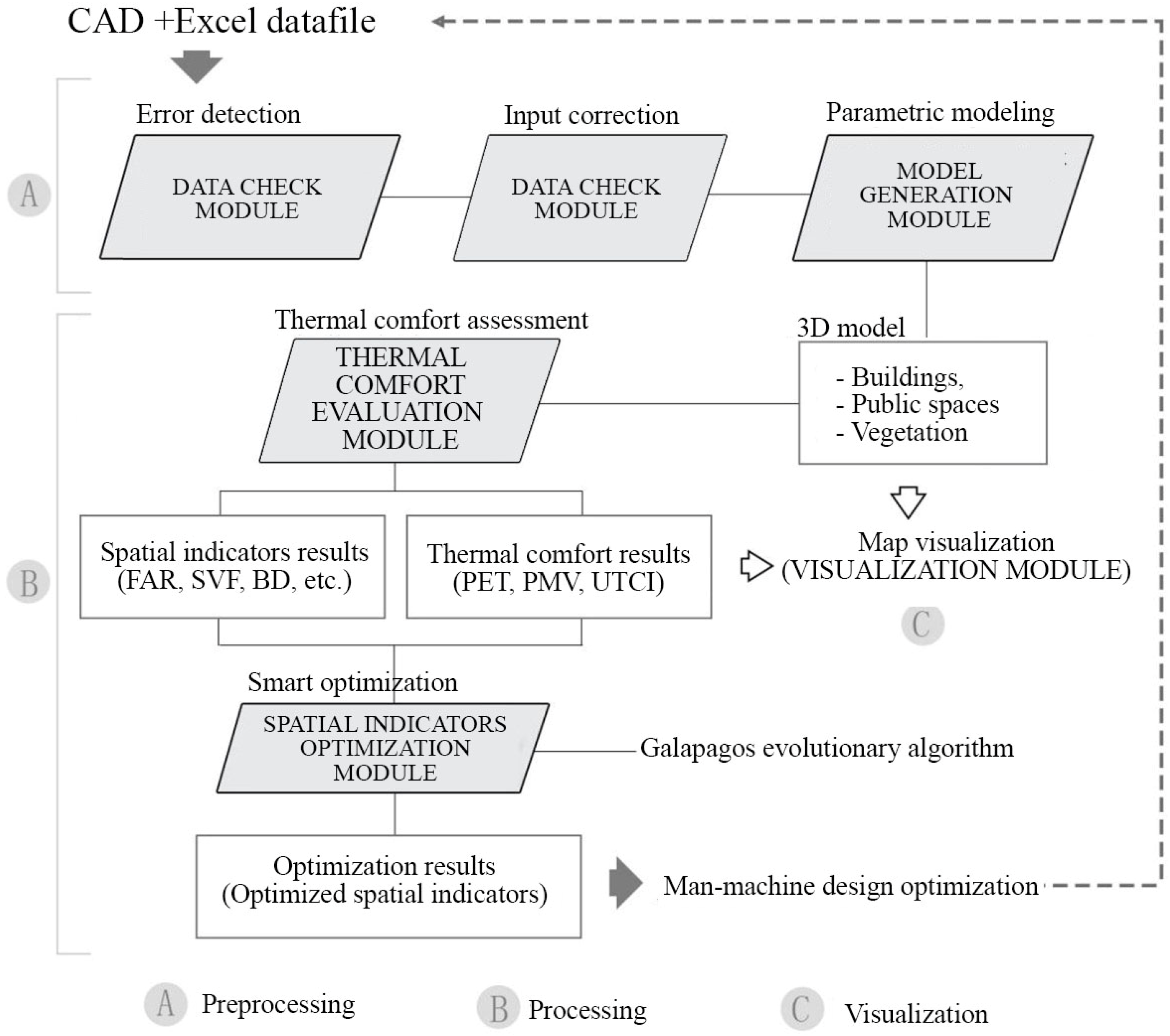
The automated assessment and optimization workflow presented in this paper is constructed to implement mainly three functions reflected in the overall structure schematized in Figure 2: (A) 3D model preprocessing, (B) processing and evaluation and (C) output visualization.

2.2.1. Model Preprocessing

The model preprocessing consists of executing two main tasks: (1) the CAD checking, which ensures that the input geometries are accurate and clean before processing, and (2) the model generation of the study area based on the input CAD geometry and an Excel datafile. The model preprocessing block executes two tasks: (3) the model consistency verification and (4) the spatial information collection.
(1)
CAD checking
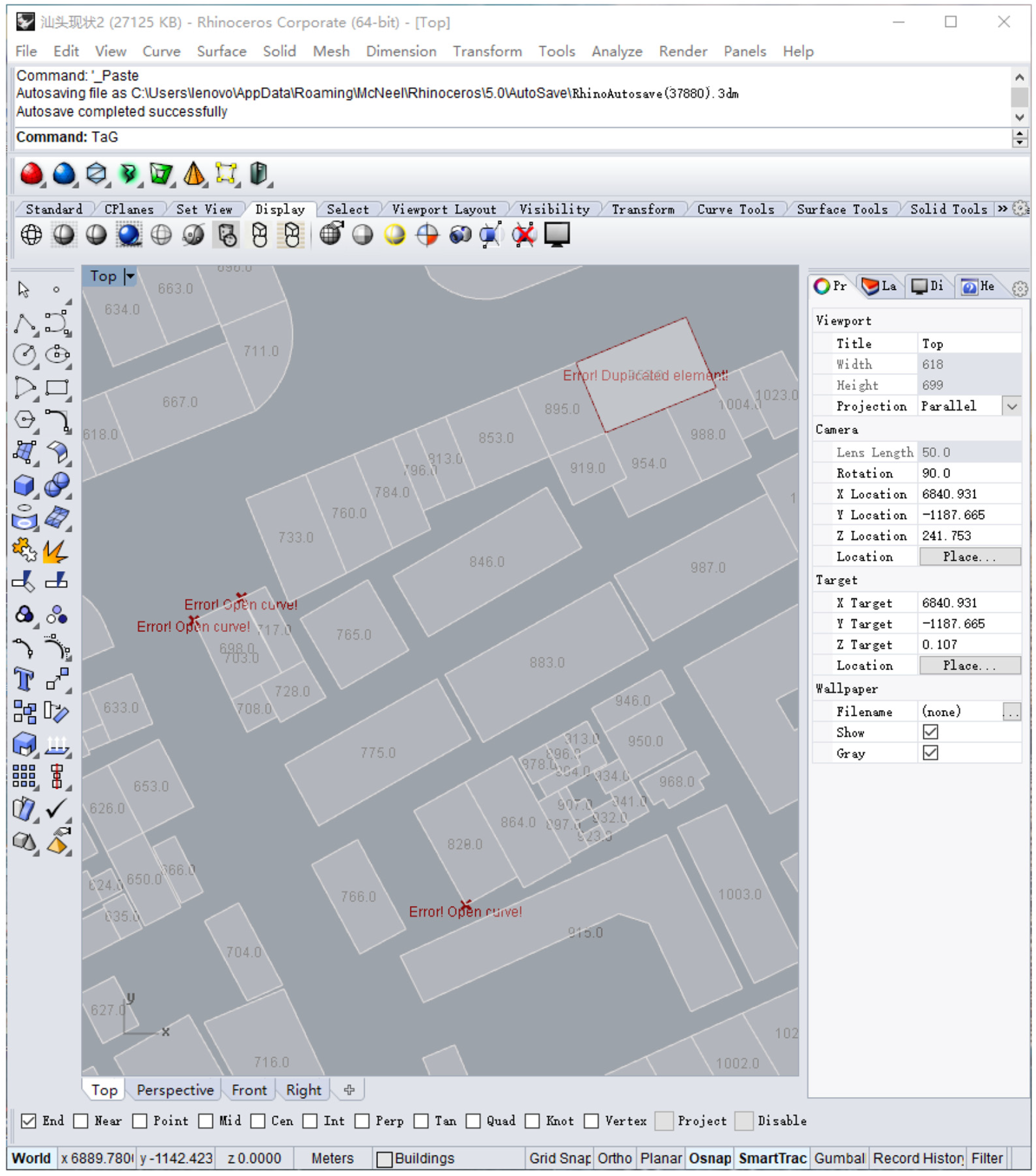
The input 2D geometry can be imported into Rhino3D in dwg, dxf or similar formats. In practice, such files may incorporate errors such as duplicates, overlaps or element type inconsistencies that are quite visually imperceptible in CAD software such as AutoCAD, but will induce reading errors or miscalculations in Grasshopper3D. The CAD checking script is thus built to verify the input geometries and clean potential errors such as overlaps, duplicates, open curves, etc., before the evaluation (Figure 3).
(2)
3D model generation:
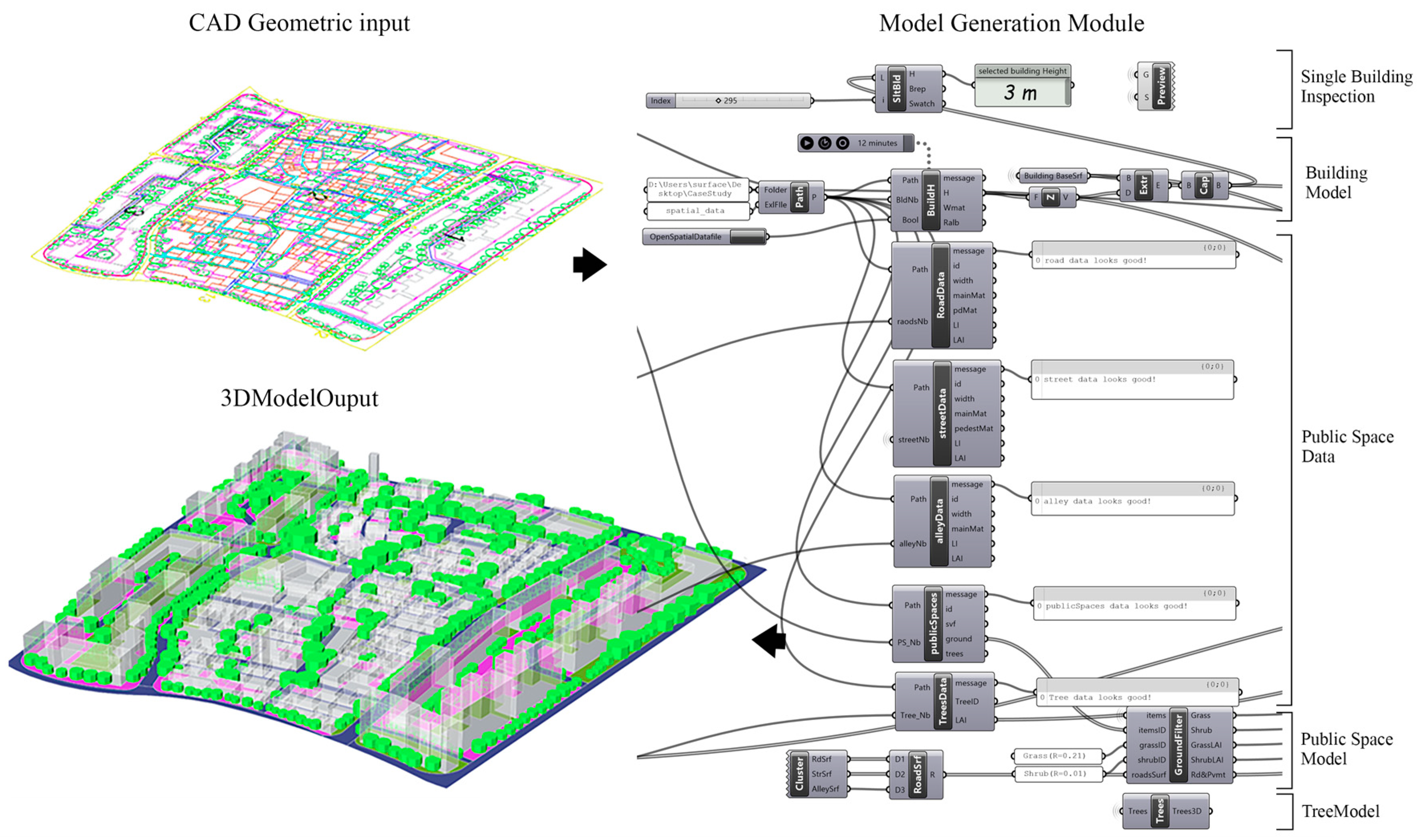
In the input CAD file, buildings, courtyards, public squares, roads and trees are represented in polylines or surfaces. These geometries are associated with their corresponding attributes from the input datafile to generate the 3D model. For example, the building contours are extruded by a z-vector, the value of which is defined by the height values from the datafile. Public space geometries are input either as closed curves or surfaces from the same layer. Depending on the keyword attribute describing their respective ground material, pavements, grass or shrubs are filtered and assigned predefined color/materials. From the input CAD file, trees are represented as 2D circles with radiuses varying according to the crown size. In Grasshopper 3D, the 3D trees are generated either by assigning predefined tree models placed at the center of the 2D circles, or by auto-generating simplified cylinders with sizes varying according to the circles’ radiuses. An illustration of 3D model output is shown in Figure 4.
(3)
Consistency verification:
The consistency verification basically ensures that the generated 3D model corresponds to the intended design. Inconsistencies may occur during the 3D model generation typically because of a mismatch between the order in the list of geometries as read by Grasshopper 3D and the order in the list of attributes read from the datafile. Two measures are taken against such inconsistencies: pre-input identification and post-input correction. The pre-input identification imposes the order of geometry lists in Grasshopper 3D by numbering the centroids of each geometry (different urban elements on different layers) and writing them into a blank datafile as their respective ID numbers. All relevant spatial data are filled in following this “imposed” order to avoid list mismatches when spatial data are read into Grasshopper 3D. Post-input corrections of the datafile may be necessary, typically in cases of missing data or data format errors, which may cause data mismatch incrementally. In such cases, the model generation script would display error messages specifying the spatial element where the error occurred and its ID number. For example, “Datafile error Building N°100″ would mean that the input datafile has either a missing value or a format error for building N°100. These data checks are conducted through custom components each named after the corresponding spatial elements (buidH, roadsData, StreetData, AlleyData, etc.). Those same components conduct the spatial information collection.
(4)
Spatial information collection
Computing thermal environment-related spatial indicators is crucial to the evaluation work presented in this paper, and the ultimate goal of the virtual model preprocessing is to retrieve data describing thermal comfort-related factors such as buildings, pavements and vegetations (grass, shrub and trees), etc. These data are retrieved from two sources: the geometries and the attributes. The geometric data include 3D buildings (Brep/Mesh), pavements (Surface/Brep) and trees (Curve/Brep/Mesh) which are virtually generated in Grasshopper 3D and visualizable in the Rhino viewport. Each geometric element is identified with an ID number in the same order as their corresponding lists in Grasshopper 3D. The attribute data include these ID numbers and their corresponding descriptions of ground materials, wall materials, leaf area density values (LAI) of trees, grass or shrubs, etc. Both the geometries and the attributes collected at this stage will serve as the main inputs for the next stage (processing and evaluation).

2.2.2. Processing and Evaluation

Taking the 3D space model generated and its associated information as input, the processing and evaluation block’s purpose is to automatically generate an evaluation of the thermal environment using a predetermined prediction model. Three steps are proposed in this paper: (1) calculation grid generation, (2) spatial indicators and thermal comfort calculations, and (3) sensitivity analysis and thermal comfort optimization.
(1)
Calculation grid generation
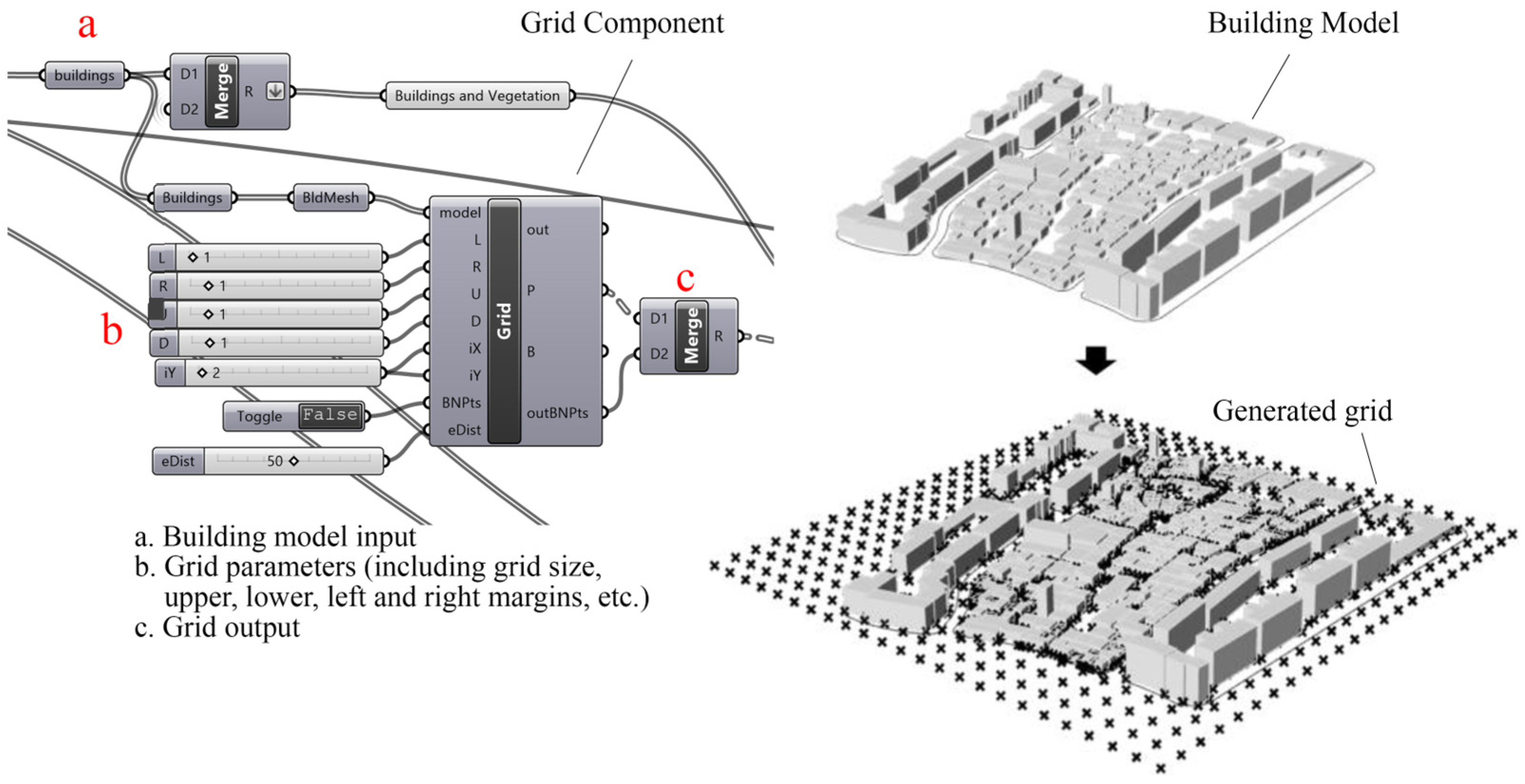
The calculation grid is an important element in the automated workflow proposed in this paper; its resolution determines the overall accuracy of the evaluation results. In principle, finer grids will lead to more precise results because smaller spaces could be covered and wider grids may fail to grasp the details of the urban form and environment. It is important to notice that the calculation grid also determines the overall computing time; finer grids mean more computing points and longer computing time. It is therefore necessary to balance computing time and precision, for which purpose a grid component (Figure 5) is designed into the script, taking as inputs the 3D model mesh, and grid parameters (L, R, U, D, iX and iY). L, R, U and D stand for the number of grids added, respectively, to the left, right, up and down the model plane. iX and iY stand for the size of each grid in the x and the y direction, respectively. Once generated, the grid is sent to the thermal comfort evaluation module (described in the following paragraphs), where a Boolean input, “Estimate”, launches the estimation of the time lag required (the result is displayed in a pop-up message). Of course, the workflow ensures greater spatial accuracy with finer grids. This implies that the trade-off for higher accuracy is the increased time-lag (diminished responsiveness). Therefore, the grid component leaves it to the user to decide on the time lag while quick-testing design ideas.
(2)
Spatial indicators and thermal comfort evaluation
1.
Spatial indicators
The spatial indicators are indispensable for thermal environment evaluation works and the specific indicators computed may depend on the prediction model used. Even though the main point in this paper is not about proposing a particular thermal environment prediction model, the spatial indicators incorporated in the script are well-documented urban-planning-related and thermal-comfort-influencing indicators such as sky view factor (SVF), floor area ratio (FAR), building height (BH), wall area ratio (WAR), building density (BD), green plot ratio (GnPR) and pavement area ratio (PAR). The selection of these spatial indicators is not only supported by an extensive literature review but is also a part of another study focused on developing thermal comfort prediction models in historical urban areas in Guangdong province, China. In this paper, the authors place emphasis on showcasing the calculation process of spatial indicators and their place in the overall automation workflow. The spatial indicator calculation formulas are shown in Table 1.
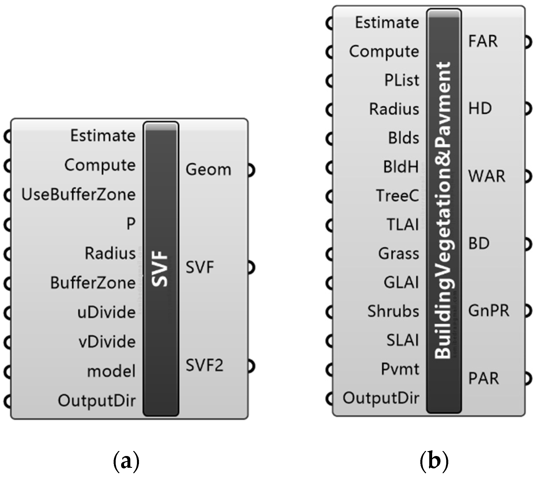
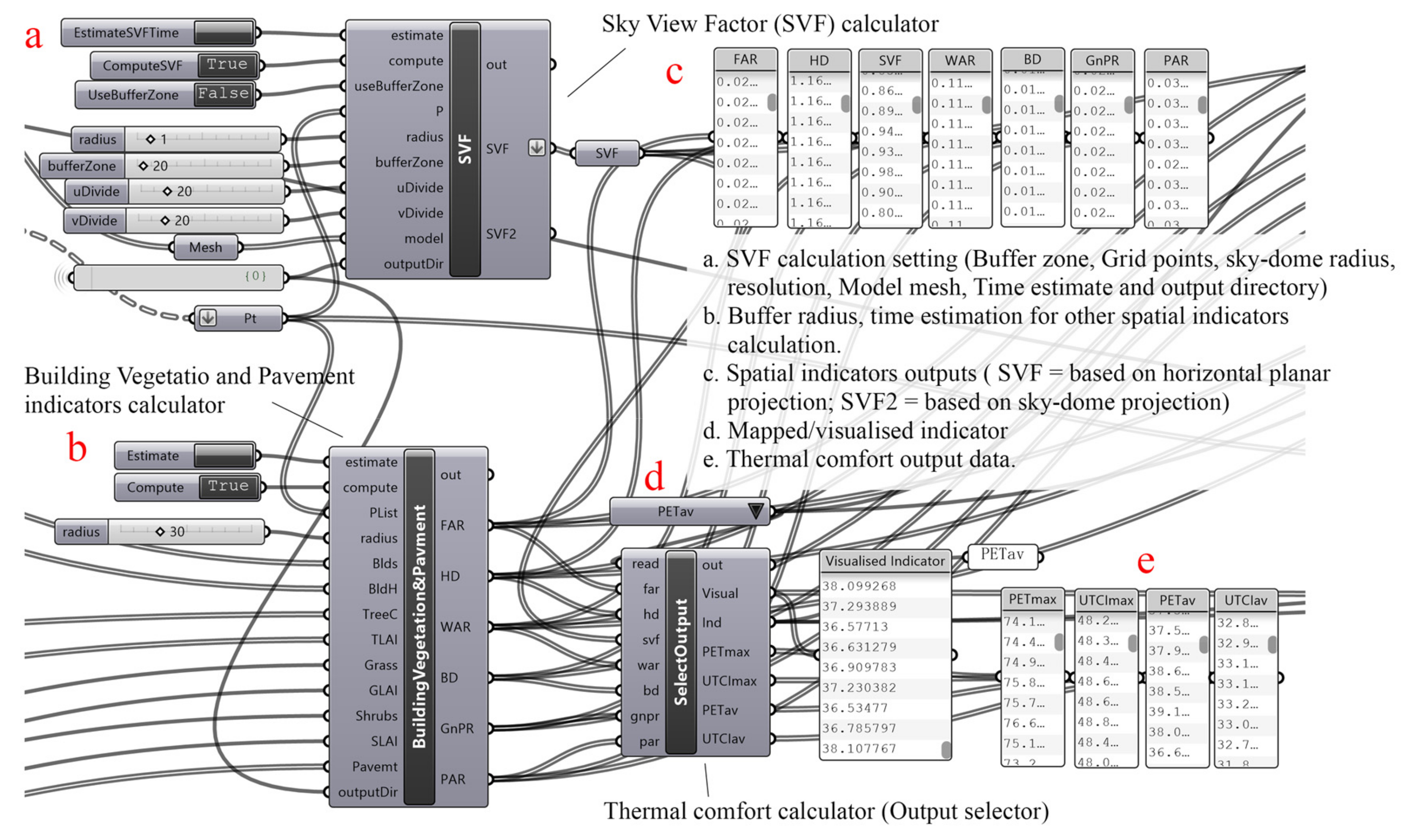
Two custom components, as shown in Figure 6 (SVF and BuildingVegetation&Pavement), were developed to handle the calculation of the spatial indicators based on the input model, the calculation grid points (P) and additional parameters such as radius, u-resolution (uDivide), v-resolution (vDivide) and output directory (outputDir). The radius defines the computation zone of the spatial indicators (SVF, BH, WAR, BD, GNPR, PAR) at each grid point; buildings and other urban elements beyond the computation zone are excluded from the calculation. uDivide and vDivide define the resolution of the sky globe while computing SVF. Other inputs such as the 3D Buildings (Bld), the vegetation models and their respective LAI values (trees, TLAI, Grass, GLAI, shrubs, SLAI) and pavements are spatial information directly collected from the urban model at the previous stage. When activated, the Boolean input, “Estimate”, displays in a pop-up message the time lag during the computation. At the specified output directory (Dir), an Excel file is automatically created where all output data, spatial indicator values and thermal comfort values are saved after computation.
2.
Thermal comfort evaluation
Thermal comfort evaluation in this case is handled by a custom component, as shown in Figure 7 (SelectOutput), which inputs the lists of spatial indicator values computed across the grid and outputs the predicted values of thermal comfort indices such as PET and UTCI. The application of the workflow presented in this paper is not limited to a certain thermal comfort index or a particular thermal environment prediction model. The appropriate prediction model is to be selected according to the suitability to the study area and the climate zone. The read input allows one to select the data to be visualized (visual) after calculation, either spatial indicators or the predicted thermal comfort index.
In this study, the following regression models of PET and UTCI were used to estimate thermal comfort based on the above-described seven spatial indicators (Equations (1)–(4)).
P E T m a x = 4.685 × F A R + 2.863 × W A R + 18.934 × S V F 1.071 × H D   + 0.093 × P A R × 100 + 0.051 × B D × 100   0.002 × G n P R × 100 + 58.703
U T C I m a x = ( 1.735 × F A R ) + ( 0.702 × W A R ) + ( 4.357 × S V F ) ( 0.261 × H D )   + ( 0.049 × P A R × 100 ) + ( 0.043 × B D × 100 )   ( 0.005 × G n P R × 100 ) + 44.606
P E T a v = 7.122 × F A R + 0.261 × B D + 0.1 × G n P R + 0.257 × P A R     + 3.489 × W A R + 1.771 × H D + 14.43 × S V F + 25.905
U T C I a v = 2.451 × F A R + 0.11 × B D + 0.051 × G n P R + 0.125 × P A R     + 1.378 × W A R + 0.497 × H D + 3.145 × S V F + 30.219
These regression models were obtained by processing extensive data sets of SVF, BH, WAR, BD, GNPR and PAR collected in more than 63 historical cities in Guangdong province, as well as the ENVI-met simulations of PET and UTCI for the same calculation points throughout the 63 historical areas. The regression analysis conducted in SPSS then yielded the three prediction models presented in Equations (1)–(4).
  • Sensitivity analysis and thermal comfort optimization
The importance of the thermal environment evaluation, particularly in the process of an urban renewal project, is not only to capture the thermal performance of the existing urban environment, but more importantly, the evaluation work should provide specific instructions for the improvement and optimization of the thermal environment. For that purpose, this paper proposes to conduct an optimization of the relevant spatial indicators (building density, floor area ratio, sky view factor, green plot ratio, etc.) preceded by a sensitivity analysis on the spatial indicators to determine the most efficient ones for optimization. The sensitivity rate i δ is determined by Equations (5) and (6):
P E T i δ = P E T I 1 + I i + δ + + I 7 P E T ( I 1 + I i + + I 7 ) δ
U T C I i δ = U T C I I 1 + I i + δ + + I 7 U T C I ( I 1 + I i + + I 7 ) δ
where
i δ represents the sensitivity of the spatial indicator I i to PET and UTCI;
δ represents a given amount of change to the value of I i ;
P E T ( I 1 + I i + δ + + I 7 ) and U T C I ( I 1 + I i + δ + + I 7 ) represent the improved values of PET and UTCI when the current value of I i is changed by  δ , the other spatial indicators remaining unchanged;
P E T ( I 1 + I i + + I 7 ) and U T C I ( I 1 + I i + + I 7 ) represent the current values of PET and UTCI.
When the spatial indicator (Ii) is negatively correlated with the thermal comfort indices (PET and UTCI), δ > 0, and when (Ii) is positively correlated with the comfort, δ < 0, due to the linear relationship between the spatial indicators and PET/UTCI, if a spatial indicator (Ii) is improved by δ, then P E T i δ > 0 and U T C I i δ > 0 indicate a reduction of heat stress.
Depending on the correlation of I i to PET and UTCI, the improvement rates are calculated with δ = L I i I i or δ = L I i I i . P E T i L I i I i , and U T C I i L I i I i are calculated when the indicator I i is positively correlated with PET and UTCI, L I i being the lowest acceptable value of I i ; likewise, the improvement rates P E T i H I i I i and P E T i H I i I i are calculated when the indicator is negatively correlated to PET and UTCI, H I i being the highest acceptable value of I i . By using the value δ = L I i I i or δ = H I i I i (which, in each case, correspond to the magnitude of improvement of I i from its current value to its optimal value), the model ignores indicators that already have values beyond the optimal boundaries and only detects the indicators that have a potential for thermal comfort improvement.
Following that logic, at each grid point, the sensitivity calculator runs this analysis for the seven spatial indicators (SVF, BH, WAR, BD, GNPR, PAR) which in the end are ranked according to the sensitivity level of each one of them. A calculation is then conducted of the number of recurrences across the calculation grid of each indicator occurring as the most sensitive indicator. This recurrence number is then ranked to yield an overall ranking which determines the adjustment of the design parameters before the genetic optimization; indicators with the highest recurrence as the most sensitive are given priority.
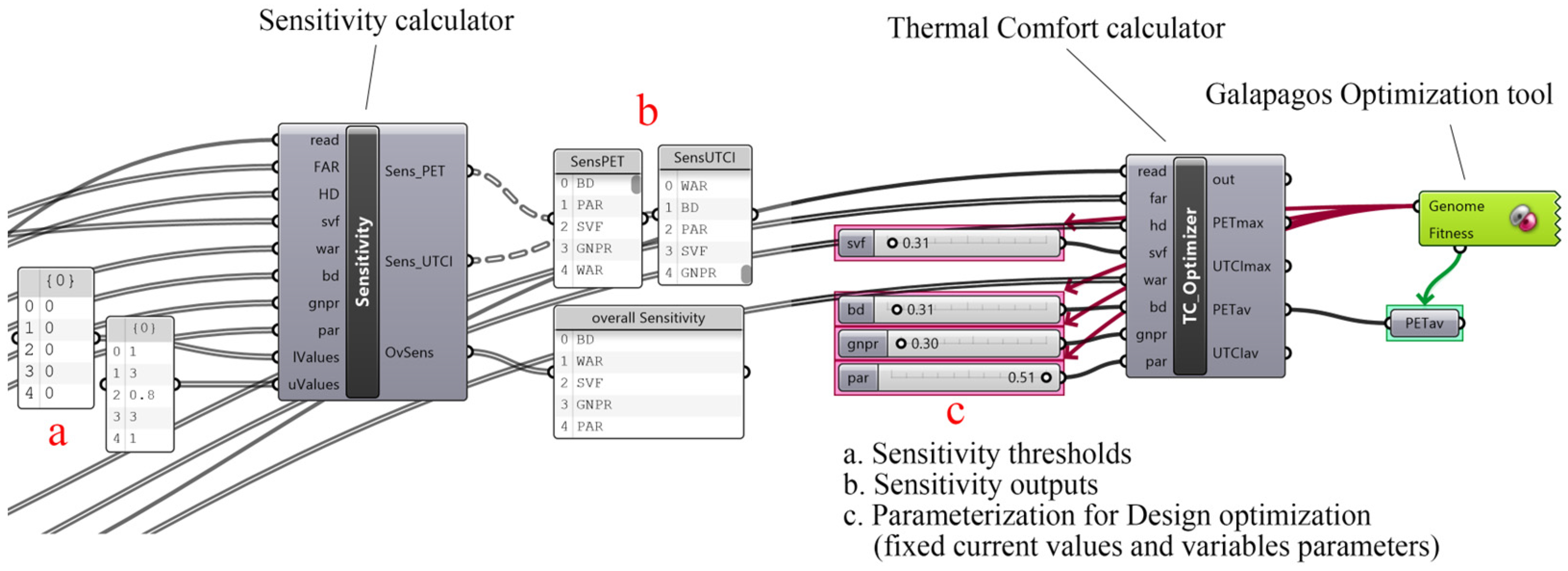
Within the Grasshopper script (Figure 8), the Sensitivity component is built to execute the above-described logic and output Sens_PET and Sens_UTCI as the ranked list of spatial indicators according to their sensitivity to thermal comfort improvement. The OvSens is the overall ranking computed as the average rank of each indicator, considering both Sens_PET and Sens_UTCI.
After that, the optimization is computed using the evolutionary algorithms of the Grasshopper self-incorporated Galapagos tool where the spatial indicators are set as the genes and either PET or UTCI as the fitness. Considering the results of the sensitivity analysis and other project specifications and goals, some spatial indicators can be set as genes for optimization while others will conserve their current values, meaning that either those current values are satisfying regarding project specifications, or they are intentionally not considered for optimization.

2.2.3. Output Visualization

Visualization is an important and indispensable part of the designer’s work process, and the practicability that Grasshopper offers for urban designers is the friendliness not only of the visual scripting but also the responsive and live visualization of Grasshopper data in the Rhino viewport. The workflow proposed in this paper uses this capability to achieve an instant visualization of not only the virtually generated urban model, but also the spatial distribution of relevant output data from the various spatial indicators calculated to the potential thermal environment as resulting from the prediction model. The general layout of the visualization script (Figure 9) is composed of three parts with three main custom components: The first, OutputExtremes, defines the boundary values for the data visualized. The second, the ColoredMap, generates the actual map with predefined color scales assigned to each indicator (by the Colors&Legend component). The third, Map Saver, saves the map currently visualized in the Rhino viewport to the specified working directory.

3. Implementation Case

The workflow described in the previous sections was applied to the evaluation of outdoor thermal comfort in the historical urban center of Shantou city in Guangzhou. In the following section, we present the localization of the study area, the existing urban environment, the evaluation of the current spatial descriptors and the thermal comfort outputs generated by the Grasshopper script. In addition, the results of the sensitivity analysis and the optimization conducted on the spatial indicators based on outdoor thermal comfort performance are presented.

3.1. Area Location

Shantou is located in eastern Guangdong between the latitudes 23°0233 and 23°3850 N and longitudes 116°1440 and 117°1935 E. The city is located at the mouths of the Han, Rong and Lian Rivers. Shantou is a prefecture-level city on the eastern coast of Guangdong, China, with a total population of 5,504,600 and an administrative area of 2.199 km2. Shantou is a significant city in Chinese 19th-century history as one of the treaty ports established for Western trade and contact. The city also was one of the original special economic zones of China established in the 1980s. Xiaogongyuan, “the small park”—which is the specific study area in this paper—is located in the old urban center of Shantou (Figure 10). The “Small Park” was the historical commercial center of the city; it is the core landmark and the cultural symbol of the old urban area. Pedestrian outdoor comfort is an important concern in such areas because of their touristic importance.

3.2. Existing Stage

According to the provincial classification of historical urban areas, the study area is covered by three main zones (Figure 11a): the preservation zone (in red), the controlled construction zone (in blue) and the style coordination zone (in green). This zoning is reflected in the existing urban fabric. For the outdoor thermal comfort assessment, a 2D CAD file (Figure 11b) was prepared and uploaded in Rhino as well as an Excel datafile which attributes building heights, pavement materials, grass and shrub to geometric elements in the CAD file. Then, the model generation module of the Grasshopper script actually generated the 3D model of the study area (Figure 11c). As perceivable in the generated model, the preservation zone is characterized by low-rise buildings and a relatively high density. In fact, these are old traditional building blocks separated by narrow streets and alleys. The controlled construction zone has a mix of a few renovated old constructions and new middle-rise buildings. The style coordination zone is marked by new high-rise buildings and more open public spaces, which link this historical center to the rest of the city developed around it harmoniously. In addition to urban geometry features, the study area is globally characterized by a low vegetation cover while ground pavements cover almost every outdoor space.

3.3. Spatial Descriptors and Thermal Comfort Outputs

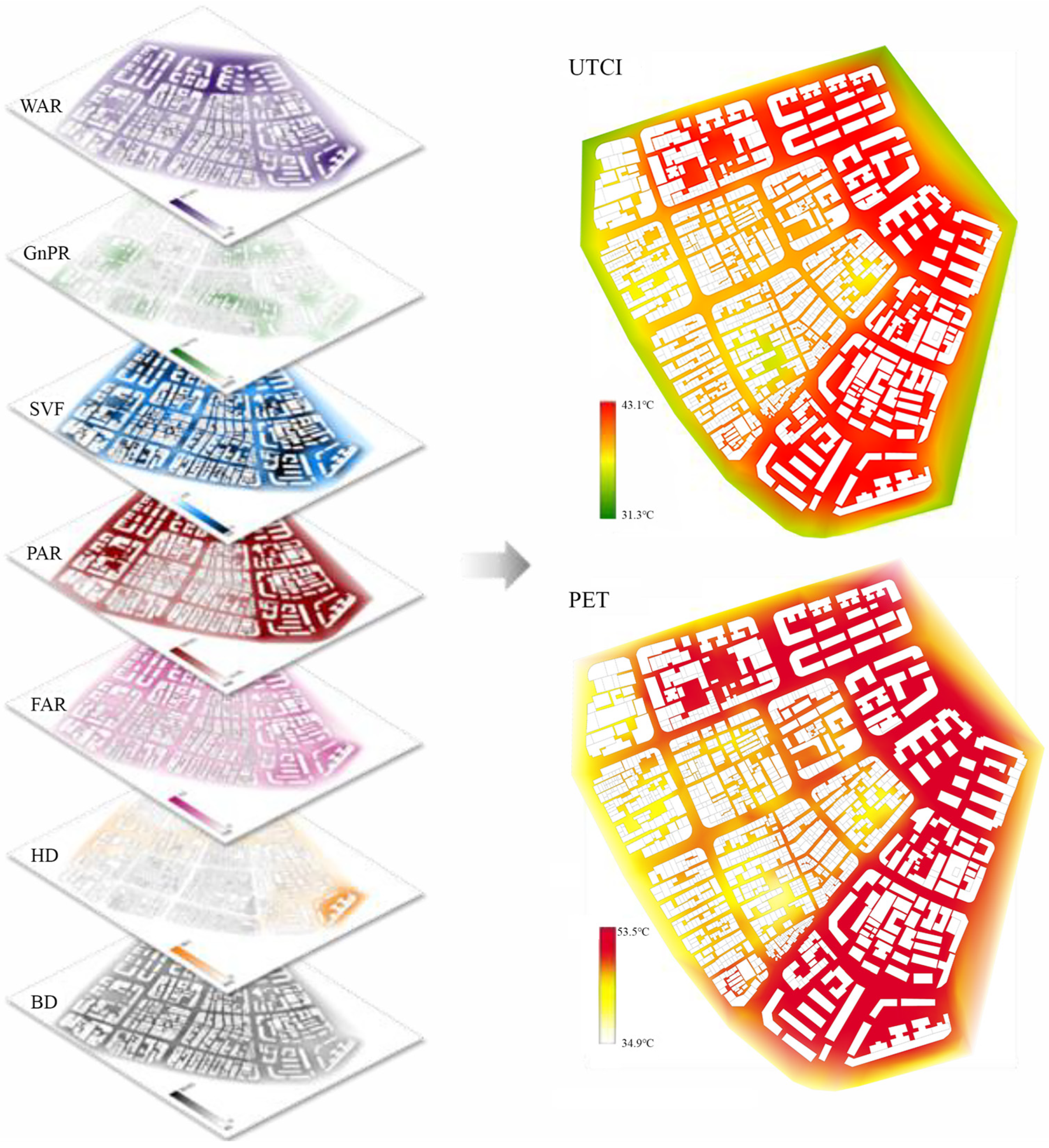
The seven spatial indicators (SVF, FAR, HD, WAR, BD, GnPR, PAR) presented earlier in the methodology, as well as PET, were computed for the study area over a 4 m × 4 m point grid, and the calculated average values of spatial indicators were 0.63, 2, 2.08, 1.75, 0.47, 0.64 and 0.51 for SVF, FAR, HD, WAR, BD, GnPR and PAR, respectively. The output PET and UTCI values, respectively, varied between [34.9 °C, 53.5 °C] and [31.3 °C, 43.1 °C], with an overall concentration of heat stress in the newly constructed zones, characterized by relatively important floor area ratio, high pavement area ratio and less vegetation cover (Figure 12).

3.4. Sensitivity Analysis and Optimization

3.4.1. Sensitivity Analysis

The sensitivity analysis was calculated on the same 4 m × 4 m grid as the spatial indicators and the thermal comfort indices. The results for this case study are presented in the following Table 2, indicating that the optimization of the pavement area, followed by the building footprint, the green plot area and the sky view factor, will have the most effect on thermal comfort improvement. Next, the optimization settings will be based on this indicator ranking alongside other project realities.

3.4.2. Optimization

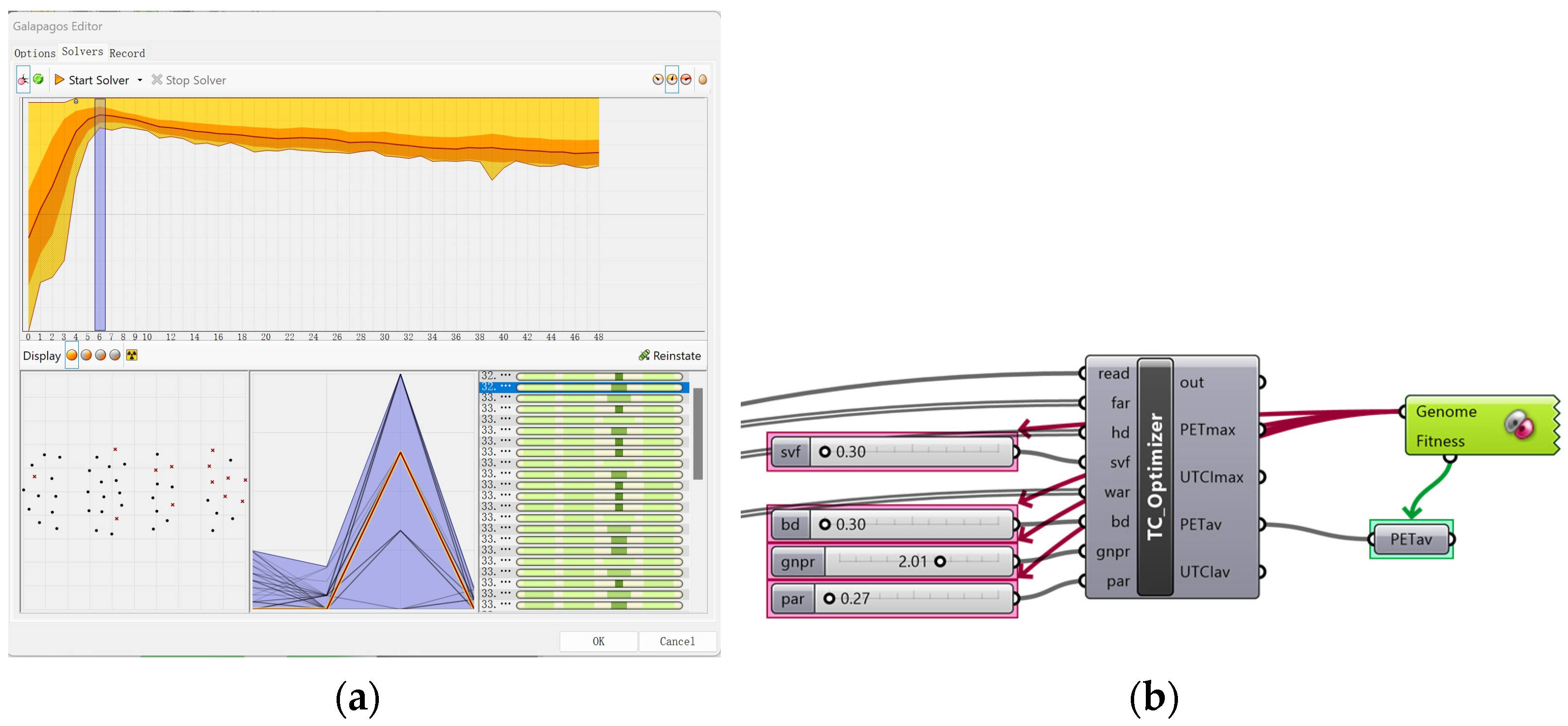
One can notice that the resulting ranks of spatial indicators, as obtained in this case, have stayed the same for both PET and UTCI. Since the optimization process for either PET or UTCI is the same, the authors chose to conduct an optimization of PET (the assumption being that the optimization of PET leads to the optimization of UTCI and vice versa). While the PET output was set as the fitness, the most sensitive spatial indicators were set as the genomes. The evolutionary algorithm then determined overall thermal improvement strategies through the best combination of ground pavement (PAR), building density (BD), vegetation cover (GnPR) and sky exposure (SVF). In this case, the evolutionary solver of Galapagos was used with default setting values and the minimized fitness (PET) was searched. The evolutionary solver was parameterized as follows: Max Stagnant (50), Population (50), Initial Boost (2x), Maintain (5%), Inbreeding (+75%). The genome boundaries were set between the existing state average value and the highest recorded value when the indicator was positively correlated to thermal comfort, or between the lowest recorded value and the existing average value when the indicator was negatively correlated. Thus, the PAR, BD, GnPR and SVF genomes were searched between [0.27, 0.51], [0.3, 0.47], [64%, 300%] and [0.3, 0.63], respectively.
As the evolutionary solver runs, an optimum value of PET = 32.4 °C was found around the 6th iteration as shown in Figure 13a. The evolutionary algorithm gives few scenarios of PAR, BD, GnPR and SVF combinations all with the same minimal PET = 32.4 °C. Among them, the following scenario (Figure 13) was selected in consideration of other project goals (microclimate-irrelevant) to conduct the improvement of the urban model: 0.30, 0.30, 2.01 and 0.27 for PAR, BD, GnPR and SVF, respectively. FAR, HD and WAR kept their pre-optimization values: 2.00, 2.08 and 1.75, respectively.

3.5. Urban Model Optimization and Results

Taking the spatial indicator values resulting from the evolutionary optimization as urban design goals, a new urban model was designed and input into the Grasshopper script for another round of thermal environment evaluation. The resulting PET and UTCI maps are compared in the figure below (Figure 14), alongside the corresponding 3D spatial models. Keeping the same value scale of PET and UTCI, one can observe a significant reduction in the very uncomfortable areas and an overall increase in the relatively comfortable areas.
To quantify the improvement made before and after optimization, five ranges of PET and UTCI values were considered, and the proportion of area covered by each value range was compared between the existing state and the optimized model. The results are summarized in the graph below (Figure 15), and a total reduction of 25% to 33% of extremely hot areas (PET ≥ 42 °C and UTCI ≥ 38 °C) can be observed; the areas of extreme heat having been incrementally converted into hot, warm and comfortable areas.

4. Discussions

The first question that is worth discussing in the context of this paper is the place of an automated microclimate evaluation process in comparison with the state of the art in microclimate simulation techniques. In this regard, the authors would first argue that the use of parametric/algorithmic design is gaining popularity among practitioners because platforms such as Rhino–Grasshopper help explore a great number of design options in a relatively short time.
As far as urban-scale thermal comfort evaluation is concerned, the authors also argue that the same time-saving goal that encourages the use of Rhino–Grasshopper (Honeybee, Ladybug, Butterfly, etc.) is to some extent held back by the background simulation engines (for instance, EnergyPlus engines for Honeybee and Ladybug, and the CFD-based OpenFOAM for Butterfly). The idea in this paper is therefore to bypass those “heavy” simulation engines with simple spatial-indicator-based statistical methods. It is worth noting that the purpose of this proposition is not to replace CFD simulation methods, but rather complement them by giving urban designers a choice of alternative methods to be used complementarily throughout the design process. For instance, the automation process demonstrated in this paper can be used in the middle of the urban design process to obtain a quick insight into the microclimate performance of design schemes, and eliminate low-performance options in the process (a sort of pre-optimization approach), before moving to CFD-based and energy balance simulation models which will take more time for urban-scale calculations but may arguably offer more advanced microclimate insights. For example, the ENVI-met model will simulate a wider range of microclimate data, including relative humidity, thermal radiation, vegetation transpiration, leaf temperatures, thermal comfort indices and others [73]. At this stage, only pre-optimized designs would necessitate such an in-depth analysis, thus saving a considerable amount of time.
The second important point worth discussing is the efficiency of the workflow, particularly regarding the speed of the data processing and the accuracy of the calculated metrics. On that point, the authors would argue that the efficiency of the workflow proposed in this paper requires accuracy for two types of calculations: the accuracy of the spatial indicators’ calculation and the accuracy of the thermal comfort prediction.

4.1. Spatial Indicator Accuracy

Fundamentally, the accuracy of the spatial indicators generated by the Grasshopper custom components (SVF, Building&Vegetation&Pavement) depends on the input geometries and the calculation script embedded in the custom components. The study has therefore conducted a comparison between the generated values of FAR, BD, HD, SVF, GnPR and PAR with those calculated using ArcGIS (which is a very popular and commonly program used for urban spatial analysis) under the same experimental settings. The details of the experimental setting are described as follows (Table 3).
The automation framework described above was executed in Grasshopper3D for Rhino7, and the results were validated against manually calculated results in ArcGIS v10.2. To ensure the comparability of the calculation results between both ArcGIS and the automation script, the calculations were performed at the same set of locations, in the same spatial model and using the same calculation formulas.
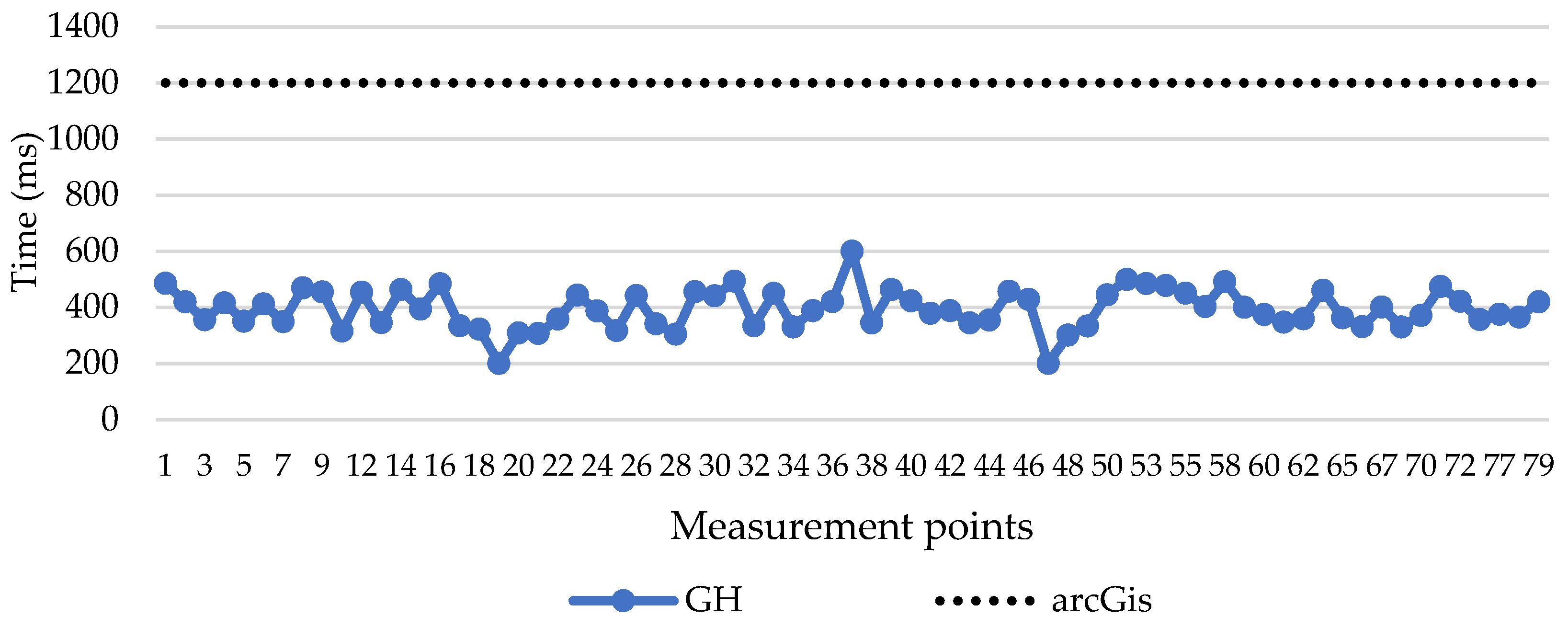
The output values were compared and the accuracy of the Grasshopper3D script was estimated, taking ArcGIS as a reference. The calculation speed in Grasshopper3D was also recorded and compared with the average calculation time in ArcGIS. The same hardware (Table 3) was used for the calculations on both platforms, one running at a time, to ensure comparability of calculation time lapse between ArcGIS and Grasshopper3D. The linear correlation between the two sets of outputs gives R2 values of 0.8839, 0.993, 0.9785, 0.8505, 0.8751, 0.9969 and 0.9917 for FAR, BD, HD, SVF, WAR, GnPR and PAR, respectively. The elapsed time for the calculation of all indicators at each measurement point was recorded and compared to the average time required for a non-automated calculation in ArcGIS. The results show that the calculations in Grasshopper can be three times faster (Figure 16).

4.2. Thermal Comfort Indicator Accuracy

The accuracy of the thermal comfort predictions is not fundamentally independent of the automation process discussed in this paper, but rather of the prediction model incorporated. In regard to that, the authors would like to emphasize that the choice of the specific thermal comfort prediction model within the automation framework proposed is still up to each project team. There is an ongoing debate about white-box prediction methods (physical mathematical and statistical models) versus black-box machine learning-based prediction methods as presented by Indira Adilkhanova et al. for Urban Heat Island prediction [74]. As they put it, “the selection of the model depends on the final objective of the study”. Assuming the same is true in the context of microclimate and thermal comfort assessment, the selection of the “right” prediction method to integrate into the automated valuation process is to be decided based on the project objectives. For detailed and holistic microclimate investigations, white-box physical models such as ENVI-met or mathematical CFD-based and energy balance models such as OpenFOAM (Butterfly plugin for Grasshopper) and EnergyPlus (Ladybug plugin for Grasshopper) are appropriate. But for overall and quick decision making, white-box statistical models such as the one used in the case of this paper or machine learning-based black-box models can all be integrated into the automation process. However, the authors deem it important to warn about the great amount of data (on-site measurements and extensive simulations) required before establishing a custom prediction model, whether based on statistical methods or machine learning.
The last important question is the validation of the prediction model. The prediction model integrated into the evaluation framework should be tested for accuracy before effective use in urban design projects. In this research, the regression models integrated into the SelectOutput component for PET and UTCI estimation were obtained and validated from an extensive field survey and numerical simulations and statistical analysis over more than 63 urban sites in Guangdong province, China, the methodology of which will be detailed in a future paper. A case of result validation is briefly described in Appendix A.

5. Conclusions

In this paper, a Rhino–Grasshopper automated workflow is proposed for the assessment and optimization of urban outdoor thermal comfort. Four main modules have been built to perform three functions: first, the 3D model preprocessing, including the input CAD and the urban data file checking; second, the outdoor thermal comfort evaluation and optimization; and finally the output visualization. The main module of the Grasshopper script is made of custom components which calculate seven spatial indicators (SVF, FAR, HD, WAR, BD, GnPR, PAR) based on the input geometries. These spatial indicators are then used to compute PET and UTCI based on three regression models obtained from the processing of extensive field data and numerical simulations. The proposed workflow is applied to the existing state of the historical urban center of Shantou city, China, to showcase the outputs of the Grasshopper script, including the 2D maps of the spatial indicators and the thermal comfort distribution across the area. This study also introduced a thermal comfort index (TCI) which normalizes and unifies the interpretation of heat stress by different thermal comfort indicators (such as PET and UTCI). In this case study, a new optimized urban model is designed based on the optimized values of spatial indicators. The optimization was conducted using the evolutionary algorithm of Galapagos, the genomes of which were parameterized according to the results of a sensitivity analysis run on the spatial indicators to detect their potential contributions to thermal comfort improvement. The comparison between the existing state and the optimized model showed a significant reduction of more than 90% for very uncomfortable areas and an increase in fairly comfortable areas from 4.93% to 17.61%, while comfortable areas increased from 0.35% to 11.97%.
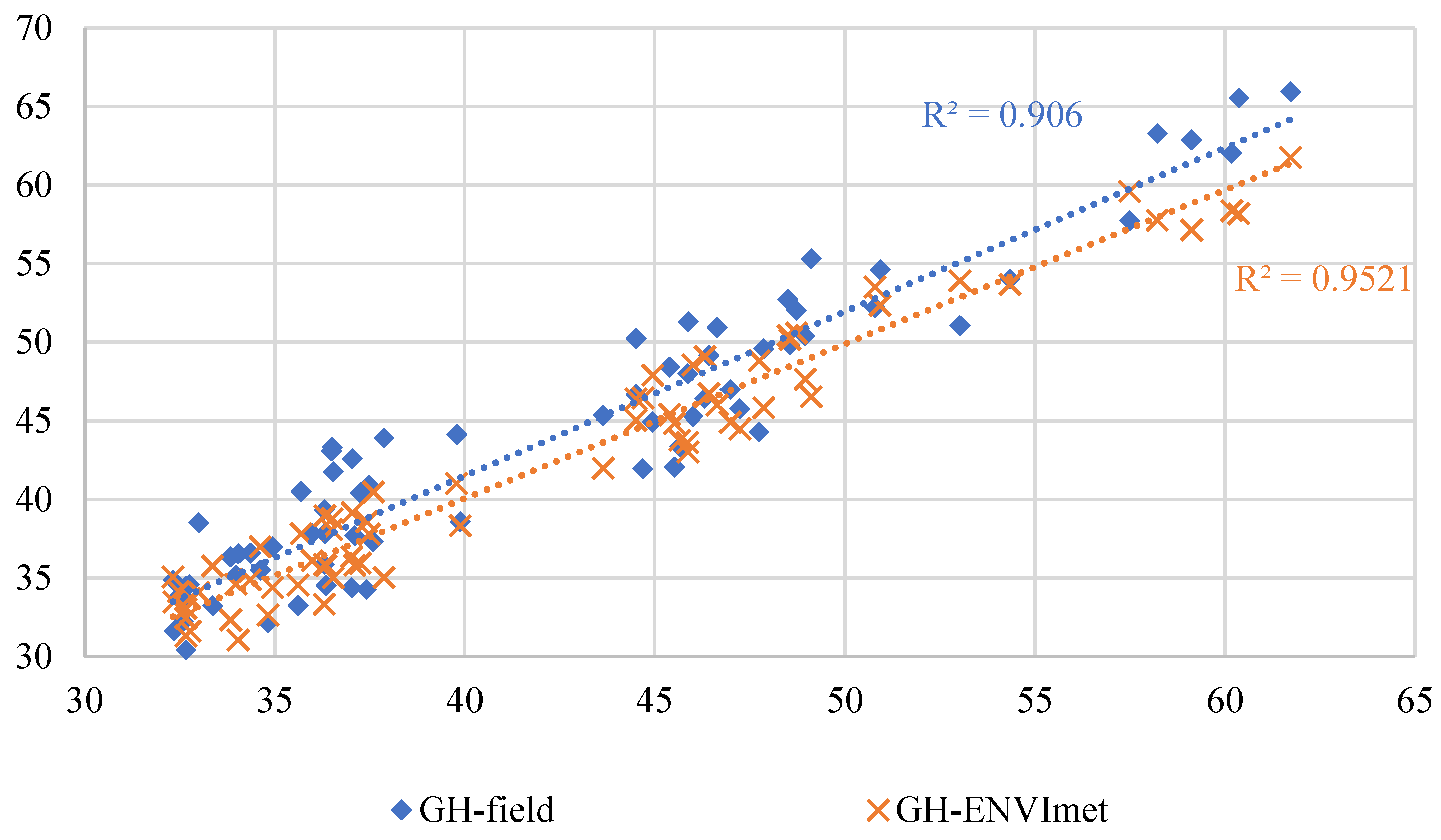
Even though the focus of this paper is not on the thermal environment prediction model itself, but rather on the automation framework, an example of model validation test was conducted on the study area, where thermal comfort estimates of PET based on field measurement data are compared with ENVI-met simulations and the predictions made in Grasshopper. The results show a relatively good degree of fitness between the three different datasets. For PET, the linear correlation resulted in r-square values of 0.906 between Grasshopper calculations and field measurements.
To achieve a responsive evaluation and smart optimization, the thermal comfort evaluation method presented in this paper is implemented with thermal comfort prediction models developed by the authors. It is important to mention, though, that the main point in the paper is still the automation method and workflow which can be adapted by using any other suitable thermal comfort prediction models, in which case the set of spatial indicators calculated can be different from those computed here.

Author Contributions

Conceptualization, K.B.B.; methodology, K.B.B.; software, K.B.B. and Z.S.; validation, K.B.B., J.Z. and J.L.; formal analysis, K.B.B., J.Z., Z.S. and J.L.; investigation, Z.S., J.L., J.Z. and B.Z.; resources, J.Z. and J.L.; data curation, K.B.B., Z.S. and J.Z.; writing—original draft preparation, K.B.B.; writing—review and editing, K.B.B., J.Z. and J.L.; visualization, K.B.B., J.Z., J.L. and B.Z.; supervision, B.Z.; project administration, B.Z.; funding acquisition, B.Z. and J.L. All authors have read and agreed to the published version of the manuscript.

Funding

This research was funded by the National Natural Science foundation of China, grant number 72174211; the Hunan Provincial Natural Science Foundation, grant numbers 2023JJ30693 and 2023JJ40728; the Hunan Provincial Philosophy and Social Science Planning Fund, grant number XSP20ZDI020; the Central South University New Teachers Research Funding, grant number 502044009; and the 2022 Hunan Province Postgraduate Research and Innovation Project, grant number CX20220123.

Institutional Review Board Statement

Not applicable.

Informed Consent Statement

Not applicable.

Data Availability Statement

The data presented in this study are available on request from the corresponding author.

Conflicts of Interest

The authors declare no conflict of interest. The funders had no role in the design of the study; in the collection, analyses, or interpretation of data; in the writing of the manuscript; or in the decision to publish the results.

Appendix A. Validation of Thermal Comfort Estimation, Taking PET as an Example
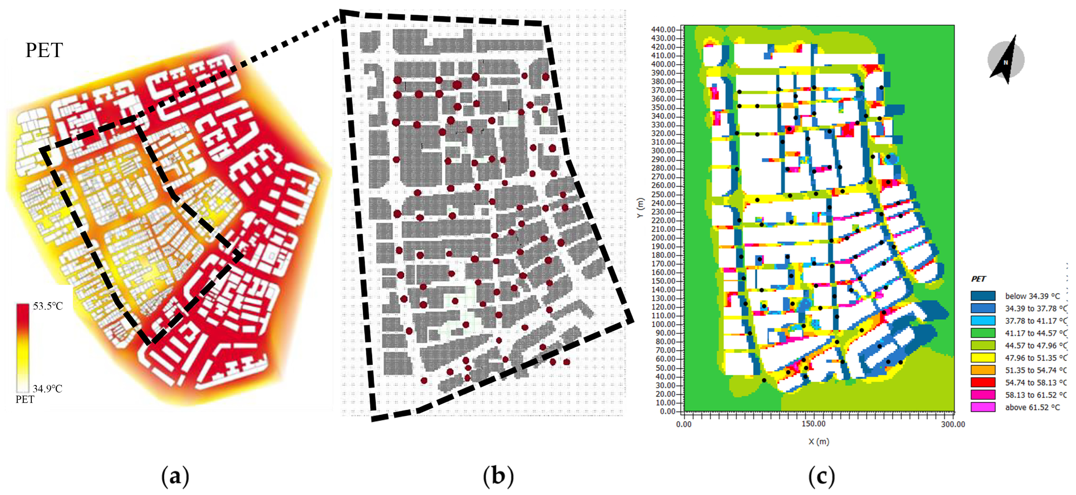
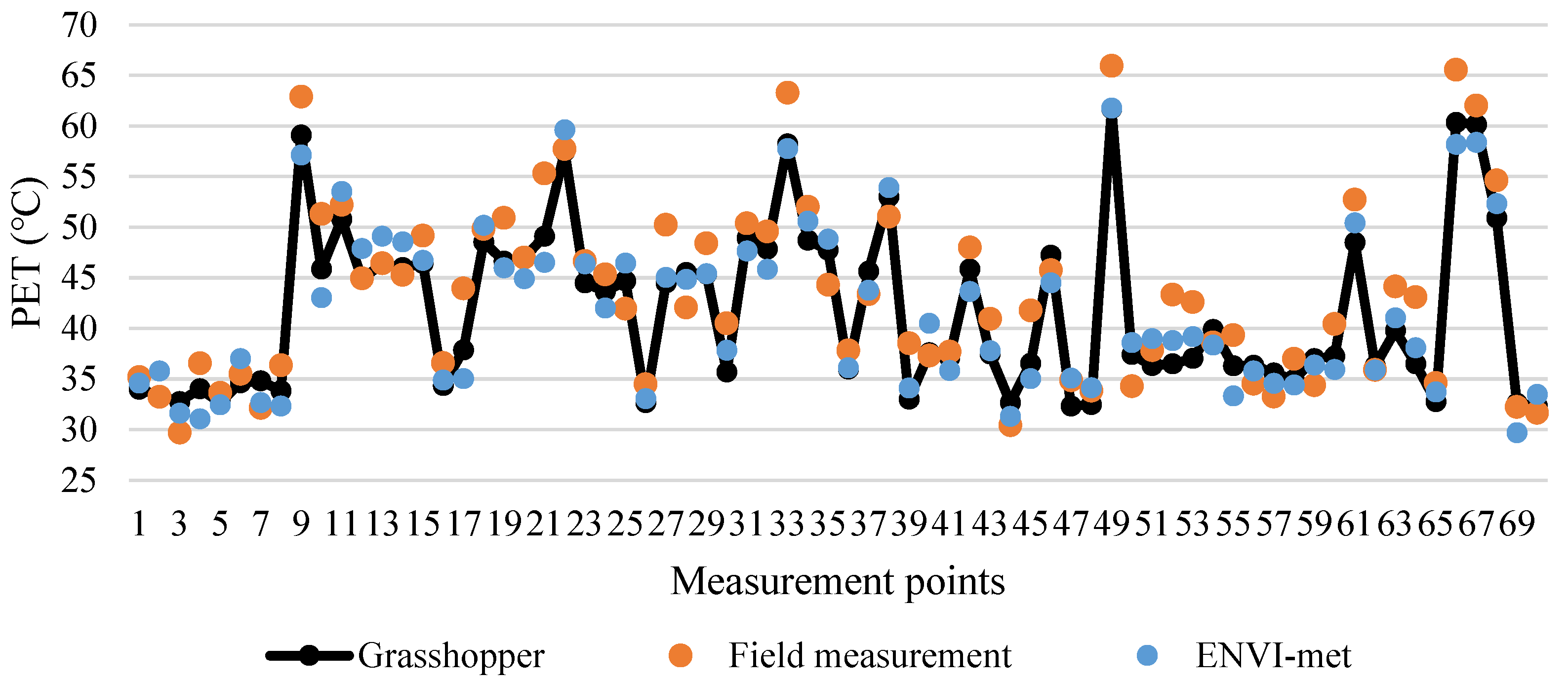
To validate the thermal comfort evaluation results, a portion of the study area (Figure A1) was isolated for a comparative analysis with ENVI-met simulation and field measurements were conducted at 70 locations (Figure A1) on the summer solstice (20 June 2021). First, the field data of air temperature, relative humidity and wind speed were input into the RaymanPro model [75] for the estimation of PET. Second, the ENVI-met model (which has been validated in a previous study in the same area [76]) was used to build a model of the same measurement area for PET simulations. Both data sets were compared with the PET predictions made in Grasshopper. The results are plotted in Figure A2, where one can notice a relatively good fitness between the three data sets (Grasshopper, field measurements and ENVI-met). Additionally, a correlation analysis was conducted in Excel to evaluate the R2 between the various datasets of PET (Figure A3). The results are relatively satisfying, with an R2 of 0.9521 between the Grasshopper prediction and ENVI-met prediction on the one hand, and 0.906 between the Grasshopper prediction and the field measurements on the other.
Figure A1. (a) Location of the validation zone; (b) ENVI-met model and measurement points; (c) ENVI-met result (PET at 1.5 m high, 3:00 p.m.).
Sustainability 15 16613 g0a1
Figure A2. PET comparison between Grasshopper simulation, field measurements and ENVI-met.
Sustainability 15 16613 g0a2
Figure A3. Linear correlation between Grasshopper simulation, field measurements and Envi-met simulation of PET.
Sustainability 15 16613 g0a3

References

  1. Santamouris, M.; Papanikolaou, N.; Livada, I.; Koronakis, I.; Georgakis, C.; Argiriou, A.; Assimakopoulos, D. On the impact of urban climate on the energy consumption of buildings. Sol. Energy 2001, 70, 201–216. [Google Scholar] [CrossRef]
  2. Department of Economic and Social Affairs, Population Division, United Nations. World Urbanization Prospects: The 2018 Revision (ST/ESA/SER.A/420). New York, USA, 2019. Available online: https://population.un.org/wup/Publications/Files/WUP2018-Report.pdf (accessed on 4 December 2023).
  3. Natanian, J.; Aleksandrowicz, O.; Auer, T. A parametric approach to optimizing urban form, energy balance and environmental quality: The case of Mediterranean districts. Appl. Energy 2019, 254, 113637. [Google Scholar] [CrossRef]
  4. Allen, M.R.; Babiker, M.; Chen, Y.; de Coninck, H.; Connors, S.; van Diemen, R.; Dube, O.P.; Ebi, K.L.; Engelbrecht, F.; Ferrat, M.; et al. Summary for Policymakers. In Global Warming of 1.5 C; IPCC: Geneva, Switzerland, 2018. [Google Scholar]
  5. Pörtner, H.-O.; Roberts, D.C.; Tignor, M.M.B.; Poloczanska, E.; Mintenbeck, K.; Alegría, A.; Craig, M.; Langsdorf, S.; Loschke, S.; Moller, V.; et al. Climate Change 2022: Impacts, Adaptation and Vulnerability, Working Group II Contribution to the Sixth Assessment Report of the Intergovernmental Panel on Climate Change. In Intergovernmental Panel on Climate Change 2022; Cambridge University Press: Cambridge, UK; New York, NY, USA, 2022; p. 3056. [Google Scholar] [CrossRef]
  6. United Nations Framework Convention on Climate Change (UNFCCC). The Paris agreement. In Paris Climate Change Conference—November 2015; United Nations: Paris, France, 2016. [Google Scholar]
  7. Alonso, C.; Martín-Consuegra, F.; Oteiza, I.; Asensio, E.; Pérez, G.; Martínez, I.; Frutos, B. Effect of façade surface finish on building energy rehabilitation. Sol. Energy 2017, 146, 470–483. [Google Scholar] [CrossRef]
  8. Heaviside, C.; Macintyre, H.; Vardoulakis, S. The Urban Heat Island: Implications for Health in a Changing Environment. Curr. Environ. Health Rep. 2017, 4, 296–305. [Google Scholar] [CrossRef]
  9. McMichael, A.J.; Wilcox, B.A. Climate Change, Human Health, and Integrative Research: A Transformative Imperative. Ecohealth 2009, 6, 163–164. [Google Scholar] [CrossRef]
  10. Deilami, K.; Kamruzzaman, M.; Liu, Y. Urban heat island effect: A systematic review of spatio-temporal factors, data, methods, and mitigation measures. Int. J. Appl. Earth Obs. Geoinf. 2018, 67, 30–42. [Google Scholar] [CrossRef]
  11. Li, X.; Zhou, Y.; Yu, S.; Jia, G.; Li, H.; Li, W. Urban heat island impacts on building energy consumption: A review of approaches and findings. Energy 2019, 174, 407–419. [Google Scholar] [CrossRef]
  12. Williams, S.; Nitschke, M.; Weinstein, P.; Pisaniello, D.L.; Parton, K.A.; Bi, P. The impact of summer temperatures and heatwaves on mortality and morbidity in Perth, Australia 1994–2008. Environ. Int. 2012, 40, 33–38. [Google Scholar] [CrossRef]
  13. Lowe, S.A. An energy and mortality impact assessment of the urban heat island in the US. Environ. Impact Assess. Rev. 2016, 56, 139–144. [Google Scholar] [CrossRef]
  14. Jamei, E.; Ossen, D.; Seyedmahmoudian, M.; Sandanayake, M.; Stojcevski, A.; Horan, B. Urban design parameters for heat mitigation in tropics. Renew. Sustain. Energy Rev. 2020, 134, 110362. [Google Scholar] [CrossRef]
  15. Lin, P.; Gou, Z.; Lau, S.S.-Y.; Qin, H. The Impact of Urban Design Descriptors on Outdoor Thermal Environment: A Literature Review. Energies 2017, 10, 2151. [Google Scholar] [CrossRef]
  16. Adelia, A.S.; Nevat, I.; Acero, J.A.; Li, S.; Ruefenacht, L. Tool Comparison for Urban Microclimate Modelling; Technical Report. D1.2.4.1; ETH Library, ETH Zürich: Zürich, Switzerland, 2020. [Google Scholar] [CrossRef]
  17. Stavrakakis, G.M.; Katsaprakakis, D.A.; Damasiotis, M. Basic Principles, Most Common Computational Tools, and Capabilities for Building Energy and Urban Microclimate Simulations. Energies 2021, 14, 6707. [Google Scholar] [CrossRef]
  18. Toparlar, Y.; Blocken, B.; Maiheu, B.; van Heijst, G. A review on the CFD analysis of urban microclimate. Renew. Sustain. Energy Rev. 2017, 80, 1613–1640. [Google Scholar] [CrossRef]
  19. Wong, N.H.; Jusuf, S.K.; Tan, C.L. Integrated urban microclimate assessment method as a sustainable urban development and urban design tool. Landsc. Urban Plan. 2011, 100, 386–389. [Google Scholar] [CrossRef]
  20. Caetano, I.; Leitão, A. Architecture meets computation: An overview of the evolution of computational design approaches in architecture. Arch. Sci. Rev. 2019, 63, 165–174. [Google Scholar] [CrossRef]
  21. Nazzarri, G.; Bier, H. Towards Circular Economy in Architecture by Means of Data-driven Design-to-Robotic-Production. In Proceedings of the 37th International Symposium on Automation and Robotics in Construction, ISARC 2020: From Demonstration to Practical Use—To New Stage of Construction Robot, Kitakyushu, Japan, 27–28 October 2020; pp. 63–66. [Google Scholar] [CrossRef]
  22. Huang, C.; Zhang, G.; Yao, J.; Wang, X.; Calautit, J.K.; Zhao, C.; An, N.; Peng, X. Accelerated environmental performance-driven urban design with generative adversarial network. Build. Environ. 2022, 224, 109575. [Google Scholar] [CrossRef]
  23. Shi, X.; Yang, W. Performance-driven architectural design and optimization technique from a perspective of architects. Autom. Constr. 2013, 32, 125–135. [Google Scholar] [CrossRef]
  24. Morgareidge, D.; Cai, H.; Jia, J. Performance-driven design with the support of digital tools: Applying discrete event simulation and space syntax on the design of the emergency department. Front. Arch. Res. 2014, 3, 250–264. [Google Scholar] [CrossRef]
  25. Lam, C.K.C.; Lee, H.; Yang, S.-R.; Park, S. A review on the significance and perspective of the numerical simulations of outdoor thermal environment. Sustain. Cities Soc. 2021, 71, 102971. [Google Scholar] [CrossRef]
  26. Taleghani, M.; Kleerekoper, L.; Tenpierik, M.; van den Dobbelsteen, A. Outdoor thermal comfort within five different urban forms in the Netherlands. Build. Environ. 2015, 83, 65–78. [Google Scholar] [CrossRef]
  27. Yang, Y.; Gatto, E.; Gao, Z.; Buccolieri, R.; Morakinyo, T.E.; Lan, H. The “plant evaluation model” for the assessment of the impact of vegetation on outdoor microclimate in the urban environment. Build. Environ. 2019, 159, 106151. [Google Scholar] [CrossRef]
  28. López-Cabeza, V.P.; Galán-Marín, C.; Rivera-Gómez, C.; Roa-Fernández, J. Courtyard microclimate ENVI-met outputs deviation from the experimental data. Build. Environ. 2018, 144, 129–141. [Google Scholar] [CrossRef]
  29. Bruse, M. ENVI-met 3.0: Updated Model Overview. 2004. Available online: www.envi-met.com (accessed on 29 September 2022).
  30. Elraouf, R.A.; Elmokadem, A.; Megahed, N.; Eleinen, O.A.; Eltarabily, S. Evaluating urban outdoor thermal comfort: A validation of ENVI-met simulation through field measurement. J. Build. Perform. Simul. 2022, 15, 268–286. [Google Scholar] [CrossRef]
  31. Caetano, I.; Santos, L.; Leitão, A. Computational design in architecture: Defining parametric, generative, and algorithmic design. Front. Arch. Res. 2020, 9, 287–300. [Google Scholar] [CrossRef]
  32. Michelle, B.; Gemilang, M.P. Bibliometric Analysis of Generative Design, Algorithmic Design, and Parametric Design in Architecture. J. Artif. Intell. Arch. 2022, 1, 30–40. [Google Scholar] [CrossRef]
  33. Frazer, J. Parametric Computation: History and Future. Arch. Des. 2016, 86, 18–23. [Google Scholar] [CrossRef]
  34. Schumacher, P. Parametricism: A New Global Style for Architecture and Urban Design. Arch. Des. 2009, 79, 14–23. [Google Scholar] [CrossRef]
  35. Delmas, A.; Donn, M.; Grosdemouge, V.; Musy, M.; Garde, F. Towards Context & Climate Sensitive Urban Design: An Integrated Simulation and Parametric Design Approach. 2018, p. 1706655. Available online: https://hal.archives-ouvertes.fr/hal-01706655 (accessed on 29 September 2022).
  36. Fink, T.; Koenig, R. Integrated Parametric Urban Design in Grasshopper/Rhinoceros 3D. In Demonstrated on a Master Plan in Vienna, Architecture in the Age of the 4th Industrial Revolution—Proceedings of the 37th ECAADe and 23rd SIGraDi Conference—Volume 3, University of Porto, Porto, Portugal, 11–13 September 2019; Sousa, J.P., Xavier, J.P., Castro Henriques, G., Eds.; 2019; Volume 3, pp. 313–322. [Google Scholar] [CrossRef]
  37. Chen, S.; Zhang, W.; Wong, N.H.; Ignatius, M. Combining CityGML files and data-driven models for microclimate simulations in a tropical city. Build. Environ. 2020, 185, 107314. [Google Scholar] [CrossRef]
  38. Elwy, I.; Ibrahim, Y.; Fahmy, M.; Mahdy, M. Outdoor microclimatic validation for hybrid simulation workflow in hot arid climates against ENVI-met and field measurements. Energy Procedia 2018, 153, 29–34. [Google Scholar] [CrossRef]
  39. Elwy, I.; Ibrahim, Y.; Fahmy, M.; Mahdy, M. Validation of outdoor microclimate simulation for hot arid regions using a parametric workflow. In The International Conference on Civil and Architecture Engineering, Architectural Engineering Department, Military Technical College, Cairo, Egypt; Military Technical College: Cairo, Egypt, 2018; Volume 12, pp. 1–11. [Google Scholar] [CrossRef]
  40. Kamel, T.M. A new comprehensive workflow for modelling outdoor thermal comfort in Egypt. Sol. Energy 2021, 225, 162–172. [Google Scholar] [CrossRef]
  41. Gardner, N.; Haeusler, M.; Yu, D. Parametricising Sound for Early-Stage Design: An Information Design Problem? Euronoise 2021, Madrid, Portugal, 25–27 October 2021. Available online: https://documentacion.sea-acustica.es/publicaciones/Madeira21/ID212.pdf (accessed on 4 December 2023).
  42. Allam, S.Z. Analogous Framework for Passive Design Strategies Using Synchronized Techniques; Validation: Dual-Skin Voronoi Pattern Façade. In Proceedings of the 2019 3rd International Conference on Smart Grid and Smart Cities ICSGSC, Berkeley, CA, USA, 25–28 June 2019; pp. 158–164. [Google Scholar] [CrossRef]
  43. Wang, X. Using CityGML EnergyADE Data in Honeybee. 2020. Available online: https://repository.tudelft.nl/islandora/object/uuid%3Afb35db7c-9af8-488c-8d0b-263b138d8fd3 (accessed on 29 September 2022).
  44. Mirzabeigi, S.; Razkenari, M. Design optimization of urban typologies: A framework for evaluating building energy performance and outdoor thermal comfort. Sustain. Cities Soc. 2022, 76, 103515. [Google Scholar] [CrossRef]
  45. Xu, X.; Yin, C.; Wang, W.; Xu, N.; Hong, T.; Li, Q. Revealing Urban Morphology and Outdoor Comfort through Genetic Algorithm-Driven Urban Block Design in Dry and Hot Regions of China. Sustainability 2019, 11, 3683. [Google Scholar] [CrossRef]
  46. Amina, N.; Fatiha, B. The using of generative algorithm aided design tool (Rhinoceros/Grasshopper/Ladybug) to control solar access in urban street of hot-arid climate (Ouargla). Revue EL-Bahith En Sciences Humaines et Sociales 2021, 13, 473–486. Available online: https://www.asjp.cerist.dz/en/downArticle/119/13/1/149365 (accessed on 4 December 2023).
  47. Touloupaki, E.; Theodosiou, T. Performance Simulation Integrated in Parametric 3D Modeling as a Method for Early Stage Design Optimization—A Review. Energies 2017, 10, 637. [Google Scholar] [CrossRef]
  48. Perini, K.; Chokhachian, A.; Dong, S.; Auer, T. Modeling and simulating urban outdoor comfort: Coupling ENVI-Met and TRNSYS by grasshopper. Energy Build. 2017, 152, 373–384. [Google Scholar] [CrossRef]
  49. Natanian, J.; Kastner, P.; Dogan, T.; Auer, T. From energy performative to livable Mediterranean cities: An annual outdoor thermal comfort and energy balance cross-climatic typological study. Energy Build. 2020, 224, 110283. [Google Scholar] [CrossRef]
  50. Koenig, R.; Knecht, K.; Miao, Y. The Development of Optimization Methods in Generative Urban Design: A Review. 2020. Available online: https://www.researchgate.net/publication/344460745 (accessed on 29 September 2022).
  51. Shi, Z.; Fonseca, J.A.; Schlueter, A. A review of simulation-based urban form generation and optimization for energy-driven urban design. Build. Environ. 2017, 121, 119–129. [Google Scholar] [CrossRef]
  52. Omid, H.; Golabchi, M. Survey of parametric optimization plugins in Rhinoceros used in contemporary architectural design. In Proceedings of the Fourth International Conference on Modern Research in Civil Engineering, Architecture, Urban Management and Environment, Karaj, Iran, 21 May 2019; Volume 17. [Google Scholar]
  53. Ibrahim, Y.; Kershaw, T.; Shepherd, P.; Elkady, H. Multi-objective optimisation of urban courtyard blocks in hot arid zones. Sol. Energy 2022, 240, 104–120. [Google Scholar] [CrossRef]
  54. Abdollahzadeh, N.; Biloria, N. Outdoor thermal comfort: Analyzing the impact of urban configurations on the thermal performance of street canyons in the humid subtropical climate of Sydney. Front. Arch. Res. 2021, 10, 394–409. [Google Scholar] [CrossRef]
  55. El Dallal, N.; Visser, F. A climate responsive urban design tool: A platform to improve energy efficiency in a dry hot climate. Int. J. Sustain. Energy 2015, 36, 738–753. [Google Scholar] [CrossRef]
  56. Duering, S.; Chronis, A.; Koenig, R. Optimizing Urban Systems: Integrated Optimization of Spatial Configurations. In Proceedings of the SimAUD, Society for Modeling & Simulation International (SCS), Vienna, Austria, 25–27 May 2020; Available online: http://simaud.org/2020/proceedings/109.pdf (accessed on 29 September 2022).
  57. Zhai, Y.; Riederer, E. Context Specific Evolutionary Design: An Analysis on Computational Abstraction of Modern Urban Complexity. In SimAUD’20: Proceedings of the 11th Annual Symposium on Simulation for Architecture and Urban Design, May 2020; Article No. 62; pp. 1–8. Available online: https://dl.acm.org/doi/abs/10.5555/3465085.3465147 (accessed on 4 December 2023).
  58. Nagy, D.; Villaggi, L.; Benjamin, D. Generative Urban Design: Integrating Financial and Energy Goals for Automated Neighborhood Layout. In Proceedings of the SimAUD, Society for Modeling & Simulation International (SCS), Delft, The Netherlands, 4–7 June 2018. [Google Scholar]
  59. Taleb, H.; Musleh, M.A. Applying urban parametric design optimisation processes to a hot climate: Case study of the UAE. Sustain. Cities Soc. 2015, 14, 236–253. [Google Scholar] [CrossRef]
  60. Brook-Lawson, J.; Holz, S. CFD Comparison Project for Wind Simulation in Landscape Architecture. Full Pap. J. Digit. Landsc. Archit. 2020, 5, 318–329. [Google Scholar] [CrossRef]
  61. Kastner, P.; Dogan, T. Eddy3D: A toolkit for decoupled outdoor thermal comfort simulations in urban areas. Build. Environ. 2022, 212, 108639. [Google Scholar] [CrossRef]
  62. Hong, T.; Lee, S.H.; Piette, M.A.; Chen, Y.; Piette, M.A. CityBES: A Web-based Platform to Support City-Scale Building Energy Efficiency. Urban Comput. 2016, 14, 2016. [Google Scholar] [CrossRef]
  63. Behboudi, N.; Butt, F.; Abhari, A. Automatic building design with genetic algorithms and artificial neural networks (WIP). In Proceedings of the 2012 Symposium on Simulation for Architecture and Urban Design, Orlando, FL, USA, 26–30 March 2012; Article 7. pp. 1–4. Available online: https://dl.acm.org/doi/abs/10.5555/2339453.2339460 (accessed on 4 December 2023).
  64. Liu, W.; Lian, Z.; Zhao, B. A neural network evaluation model for individual thermal comfort. Energy Build. 2007, 39, 1115–1122. [Google Scholar] [CrossRef]
  65. Artificial Neural Networks Based Prediction for Thermal Comfort in An Academic Classroom|IEEE Conference Publication|IEEE Xplore, (n.d.). Available online: https://ieeexplore.ieee.org/abstract/document/6828926 (accessed on 30 September 2022).
  66. Li, N.; Yu, W.; Li, B. Assessing Adaptive Thermal Comfort Using Artificial Neural Networks in Naturally-Ventilated Buildings. Int. J. Vent. 2012, 11, 205–218. [Google Scholar] [CrossRef]
  67. Wang, B.; Yi, Y.K. Developing an adapted UTCI (Universal Thermal Climate Index) for the elderly population in China’s severe cold climate region. Sustain. Cities Soc. 2021, 69, 102813. [Google Scholar] [CrossRef]
  68. Afram, A.; Janabi-Sharifi, F.; Fung, A.S.; Raahemifar, K. Artificial neural network (ANN) based model predictive control (MPC) and optimization of HVAC systems: A state of the art review and case study of a residential HVAC system. Energy Build. 2017, 141, 96–113. [Google Scholar] [CrossRef]
  69. Yoon, H.-J.; Lee, D.-S.; Cho, H.; Jo, J.-H. Prediction of Thermal Environment in a Large Space Using Artificial Neural Network. Energies 2018, 11, 418. [Google Scholar] [CrossRef]
  70. Zhang, R.; Liu, D.; Shi, L. Thermal-comfort optimization design method for semi-outdoor stadium using machine learning. Build. Environ. 2022, 215, 108890. [Google Scholar] [CrossRef]
  71. Tabadkani, A.; Aghasizadeh, S.; Banihashemi, S.; Hajirasouli, A. Courtyard design impact on indoor thermal comfort and utility costs for residential households: Comparative analysis and deep-learning predictive model. Front. Arch. Res. 2022, 11, 963–980. [Google Scholar] [CrossRef]
  72. Fard, Z.Q.; Zomorodian, Z.S.; Korsavi, S.S. Application of machine learning in thermal comfort studies: A review of methods, performance and challenges. Energy Build. 2022, 256, 111771. [Google Scholar] [CrossRef]
  73. Simon, H.; Lindén, J.; Hoffmann, D.; Braun, P.; Bruse, M.; Esper, J. Modeling transpiration and leaf temperature of urban trees—A case study evaluating the microclimate model ENVI-met against measurement data. Landsc. Urban Plan. 2018, 174, 33–40. [Google Scholar] [CrossRef]
  74. Adilkhanova, I.; Ngarambe, J.; Yun, G.Y. Recent advances in black box and white-box models for urban heat island prediction: Implications of fusing the two methods. Renew. Sustain. Energy Rev. 2022, 165, 112520. [Google Scholar] [CrossRef]
  75. Matzarakis, A.; Rutz, F.; Mayer, H. Modelling radiation fluxes in simple and complex environments: Basics of the RayMan model. Int. J. Biometeorol. 2010, 54, 131–139. [Google Scholar] [CrossRef]
  76. Zheng, B.; Bedra, K.B.; Zheng, J.; Wang, G. Combination of Tree Configuration with Street Configuration for Thermal Comfort Optimization under Extreme Summer Conditions in the Urban Center of Shantou City, China. Sustainability 2018, 10, 4192. [Google Scholar] [CrossRef]
Figure 1. Conceptual framework: (a) general framework; (b) specific framework (adapted from E. Touloupaki and T. Theodosiou [47]).
Sustainability 15 16613 g001
Figure 2. Workflow structure and data flow.
Sustainability 15 16613 g002
Figure 3. Examples of geometry errors.
Sustainability 15 16613 g003
Figure 4. Model generation module: from CAD geometric input to 3D model output.
Sustainability 15 16613 g004
Figure 5. The analysis grid calculator.
Sustainability 15 16613 g005
Figure 6. Spatial indicator calculators: (a) SVF; (b) building, vegetation and pavement indictors.
Sustainability 15 16613 g006
Figure 7. Thermal comfort evaluation module (spatial parameters and thermal comfort calculators).
Sustainability 15 16613 g007
Figure 8. Spatial indicator sensitivity and optimization module.
Sustainability 15 16613 g008
Figure 9. Results visualization module.
Sustainability 15 16613 g009
Figure 10. Location map: (a) Guangdong province; (b): Shantou municipal area; (c) the study area.
Sustainability 15 16613 g010
Figure 11. Study area: (a) the historical urban area classification, (b) the 2D model and (c) the generated 3D model.
Sustainability 15 16613 g011
Figure 12. Spatial indicators and thermal comfort outputs.
Sustainability 15 16613 g012
Figure 13. Evolutionary optimization results: (a) selected results in the Galapagos editor; (b) reinstated genome and fitness values.
Sustainability 15 16613 g013
Figure 14. Urban models and thermal environments before and after optimization: (a) current urban model, (b) optimized urban model, (c) PET map before optimization, (d) PET map after optimization, (e) UTCI map before optimization and (f) UTCI map after optimization.
Sustainability 15 16613 g014
Figure 15. Distribution of thermal stress before and after optimization: (a) PET, (b) UTCI.
Sustainability 15 16613 g015
Figure 16. Comparison between the Rhino–Grasshopper computation time per point and the average computation time in ArcGIS.
Sustainability 15 16613 g016
Table 1. Calculation method of thermal environment spatial indicators.
IndexCalculation Method
Floor Area Ratio
(FAR)
F A R = T o t a l   f l o o r   a r e a t o t a l   g r o u n d   a r e a
Building Density
(BD)
B D = T o t a l   a r e a   o f   t h e   b u i l d i n g   b a s e t o t a l   g r o u n d   a r e a × 100 %
Height Deviation of Buildings
(HD)
H D = S t a n d a r d   d e v i a t i o n   o f   b u i l d i n g   h e i g h t s
Sky View Factor
(SVF)
In Rhino–Grasshopper, rays are emitted in all directions from the measurement point and the number of rays that are not blocked by buildings is counted.
S V F = T h e   n u m b e r   o f   u n b l o c k e d   r a y s T o t a l   n u m b e r   o f   r a y s
Wall Area Ratio
(WAR)
W A R = T h e   t o t a l   a r e a   o f   e x t e r i o r   w a l l s t o t a l   g r o u n d   a r e a × 100 %
Pavement Area Ratio
(PAR)
P A R = T o t a l   a r e a   o f   h a r d   p a v i n g t o t a l   g r o u n d   a r e a × 100 %
Green Plot Ratio
(GnPR)
G n P R = L A I t r e e s   ×   A r e a t r e e s   +   L A I s h r u b   ×   A r e a S h r u b   +   L A I g r a s s   ×   A r e a g r a s s P i   ×   R 2
Table 2. Spatial indicators and their sensitivity to TCI improvement.
RankingSpatial IndicatorsSensitivity to PETSensitivity to UTCI
1PAR21.336814.1912
2BD17.272611.5060
3GNPR08.451705.7009
4SVF08.368104.6764
5FAR04.475802.8764
6WAR02.697901.6986
7HD01.010300.6343
Table 3. Experimental settings for indicator calculation (Rhino7 vs. ArcGIS10.2).
ElementsDescription
HardwareModel: HP Pavilion Gaming Desktop TG01-1XXX
Processor: Intel®/core (TM) i7-10700F CPU @ 2.9 GHz, 2.9 GHz, 8, 16 core
System: Windows10 Family edition, x64
Memory: 16.0 GB
SoftwareRhino 7 vs. ArcGIS10.2
Disclaimer/Publisher’s Note: The statements, opinions and data contained in all publications are solely those of the individual author(s) and contributor(s) and not of MDPI and/or the editor(s). MDPI and/or the editor(s) disclaim responsibility for any injury to people or property resulting from any ideas, methods, instructions or products referred to in the content.