1. Introduction
Sustainable mobility has emerged in response to the environmental and social challenges associated with urban growth and increased vehicular traffic. This paradigm seeks to transform modes of travel, promoting alternatives that reduce greenhouse gas emissions and minimize the impact on ecosystems. Research efforts have focused on a variety of fronts, from the development of more efficient and cleaner vehicle technologies to mobility-oriented urban planning. Sustainable mobility research has become an interdisciplinary and constantly evolving field, driven by the urgent need to find viable and sustainable solutions to the growing transportation demands in cities.
The most crucial research areas, revealing a diverse and complex landscape, have emerged as a crucial convergence with Intelligent Transportation Systems (ITSs), marking a transition towards more advanced and effective solutions. These systems, supported by innovative technologies such as real-time data analytics and artificial intelligence, offer unprecedented opportunities to improve traffic management, facilitate urban planning and encourage the adoption of sustainable modes of transportation.
Research and analysis of Intelligent Transportation Systems in urban areas have become essential today due to the complexity of this problem and its profound impact on society. The constant growth of the population in urban areas as well as the increase in vehicular traffic are obvious factors that require careful attention [
1].
Intelligent Transportation Systems emerge as an innovative and technological response for addressing these challenges in an efficient and sustainable manner. In their search for effective solutions to the challenges of urban mobility, they employ a variety of machine learning techniques to obtain practical applications and offer analytical approaches in the field of transportation.
Intelligent Transportation Systems use machine learning algorithms to detect patterns in vehicle behavior, such as regular congestion in certain areas or drivers’ preferred routes. This information is essential for congestion prediction, optimal route planning and real-time adaptation of traffic management strategies.
The applicability of these approaches is broad, ranging from real-time traffic management to long-term planning of transportation infrastructure. By better understanding traffic patterns and driver behaviors, intelligent systems can offer more effective solutions, such as traffic light optimization, public transport route management and the implementation of sustainable mobility policies.
In this regard, the management of vehicular traffic in urban areas is of great importance due to the constant population growth and increase in vehicles, which poses significant challenges [
2]. This management must address multiple dimensions, including environmental impact and road safety. Traffic congestion is a recurring problem that affects the quality of life of citizens.
There are challenges in managing traffic congestion such as the lack of an accurate and uniform representation of vehicle trajectory data, which makes early identification of congested areas difficult [
3]. Dispersion and incompleteness of data collection points are also common problems.
Efficient traffic management is essential for improving road flow, reducing travel time and reducing pollutant emissions. Traditional approaches may not adapt quickly to changing traffic conditions, which is essential given that congestion can vary significantly at different times of the day [
4].
Data streams, collected from various sources such as traffic sensors and GPS navigation systems, are essential for understanding the real-time behavior of vehicles and pedestrians in urban areas [
5,
6,
7]. Clustering techniques are valuable for representing these data streams effectively, allowing for the identification of traffic patterns, organization of data into clusters based on similarities and prediction of future trends in urban traffic [
8]. These techniques are fundamental for traffic planning and management tailored to the specific needs of each area.
The analysis of vehicular trajectory data streams is a widely researched area [
9], and several studies have developed clustering techniques adapted to different domains [
10,
11,
12]. The study of various approaches has proven effective in identifying sets with shared attributes in the analysis of the joint behavior of vehicles [
13,
14].
Some researchers have adapted conventional clustering methods, such as k-means [
10] and DBSCAN [
15], by adapting methods and calculations designed specifically for trajectories [
16]. Several investigations have resorted to alternative representations [
17] of trajectories such as subdivision or cell representation to improve clustering results [
18,
19].
In some cases, static vehicle analysis may be limited in its ability to capture real traffic dynamics. Because vehicle behavior can change over time [
20], dynamic analysis has become important for understanding the causes of congestion [
21]. Dynamic clustering emerges as an innovative and promising strategy. Contrary to static methods, dynamic clustering allows for continuous adaptation to changes in urban traffic. The relevance of dynamic clustering lies in its ability to capture constantly evolving mobility patterns and the identification of areas prone to congestion [
22].
In recent years, there has been an increase in artificial intelligence and machine learning approaches that add features such as memory, scalability and accuracy [
23,
24,
25]. Machine learning has proven its effectiveness by leveraging the use of historical information combined with information associated with vehicles and the road environment in which they travel [
26,
27,
28]. These combinations, enriched by the inclusion of data from Big Data, especially generated from social networks, have become an invaluable resource for detecting traffic congestion in real time [
29].
Several studies have developed methodologies and techniques for identifying congested areas accurately, using a variety of traffic and environmental characteristics [
30,
31,
32,
33].
Several proposals with combined approaches focusing on traffic congestion assessment and the use of clustering algorithms constitute a highly promising field of research [
34,
35,
36], providing an effective method for closely examining vehicular flow in different scenarios [
30,
37,
38].
The paper proposed by Almeida et al. [
39] proposes a method for traffic congestion detection considering speed, traffic flow and road occupancy and then uses clustering techniques to detect various degrees of congestion in vehicular data. The paper proposed by Reyes et al. [
40] analyzes vehicular flow by identifying speed ranges with a constant update. Although it is a simplified view of vehicular traffic flow, in many cases it is beneficial to include additional data in order to enrich the study of vehicular traffic [
41].
A detailed understanding of how congestion manifests and evolves in different environments is critical to strategically planning mobility, alleviating congestion and ensuring more efficient and sustainable traffic flow.
For the analysis of vehicle trajectory data, a variety of approaches can be seen, the most prominent of which are the application of a dynamic clustering algorithm and the evaluation of traffic congestion by means of an indicator that adapts to different areas. The combination of these perspectives presents itself as a potential and suggestive area of research, offering a comprehensive understanding for addressing vehicular flow. The combination of congestion assessment and the application of clustering algorithms may be a valuable area of study for improving efficiency and planning in urban environments.
This paper proposes a methodology to analyze vehicular flow by clustering vehicle trajectory data with GPS points. This methodology allows for an accurate representation of the data, especially useful when points are scarce. It uses clusters to detect areas of congestion patterns. The constant updating of the clusters ensures up-to-date data and real congestion management. It also uses a congestion indicator to measure traffic saturation, allowing for a dynamic view of the traffic situation in different areas.
This article is organized as follows:
Section 2 describes the proposed methodology,
Section 3 presents the obtained results,
Section 4 discusses the obtained results, and
Section 5 presents the conclusions and future lines of work.
2. Materials and Methods
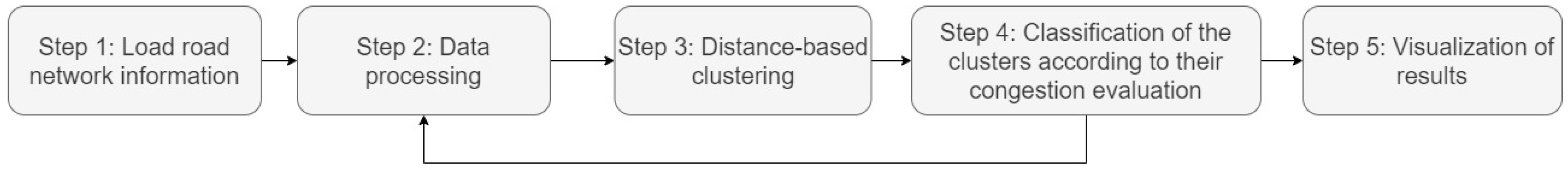
This paper presents a methodology for the identification of congestion zones based mainly on dynamic clustering. The methodology used consists of five steps illustrated in
Figure 1. In the first step, road network data information is loaded. In the second step, a GPS trajectory data stream is processed. In the third step, a distance-based dynamic clustering algorithm is used to identify areas with similar patterns. In the fourth step, areas are evaluated with a congestion indicator for further classification. In the fifth step, we proceed to generate a suitable visualization of the resulting clusters already classified. Each of these steps is described in detail below.
2.1. Step 1: Load Road Network Information
The estimation of reference data is important for ensuring the reliability of the results and for strengthening the validity and consistency of the analyses performed.
The main purpose of this step is to load into memory the relevant information on the road infrastructure in the area to be analyzed. This includes detailed data on road layout, geographical location, capacity, number of lanes and speed limits. These data will not only be used for the analysis but will also enable an effective comparison between different road sections, thus establishing a solid benchmark for detecting and assessing road congestion accurately.
The robustness of the results depends on the quality and comprehensiveness of the data collected in this step. Accuracy in the representation of the road network and thoroughness in data collection are essential for ensuring robust and reliable results in the subsequent steps of this study.
It is recommended that a monthly update process be implemented to ensure the currency and accuracy of road network data in changing urban environments. For a change in the direction of a road that modifies the dynamics of vehicular flow, for example, depending on the technological infrastructure in the source that stores the information regarding road networks, updating changes in the sources could take several days.
2.2. Step 2: Data Processing
In this step, a method is established for receiving and processing GPS points in real time or from an accessible repository. These data come from GPS-equipped vehicles or in-vehicle mobile applications. Processing is performed in microbatches at evenly distributed time intervals, called “cycles”, which represent moments in the evolution of the data streams.
At each cycle, data are accumulated in a temporal buffer, and the results of the clustering method are updated as new data are added. To address the lack of information in the trajectory data, a routing method and an interpolation method are implemented that operate simultaneously during the collection of new GPS locations.
The decision to perform routing and interpolation along with data accumulation is justified by its ability to generate an enriched and densely populated data buffer. This ensures that as the data stream progresses, it works with complete and accurate route information for each vehicle, improving the efficiency of the subsequent clustering analysis.
One of the underlying functions of this step is to mitigate the challenges associated with the presence of GPS data affected by noise and incompleteness. Routing is proposed as an effective strategy for dealing with noisy data, contributing to the cleaning and improvement of the quality of vehicle trajectory data. Interpolation is presented as a key tool for estimating missing values, allowing for a detailed representation of the observed vehicle location information. These strategies are implemented with the purpose of optimizing the accuracy and consistency of the road network data used in the clustering process.
The routing method uses the Open Source Routing Machine (OSRM) service, based on contraction hierarchies and travel time optimization. This service calculates the shortest route and generates key spatial points based on the geometry of the road networks, projecting an artificial route on the roads that the vehicle could have driven on.
The distance-based interpolation method consists of continuously estimating data values along a route with a constant interval of 5 m. These techniques are applied to complete routes in cases where there are no records for certain sections, providing a more detailed and uniform representation of the data, especially useful when collection points are scattered or incomplete.
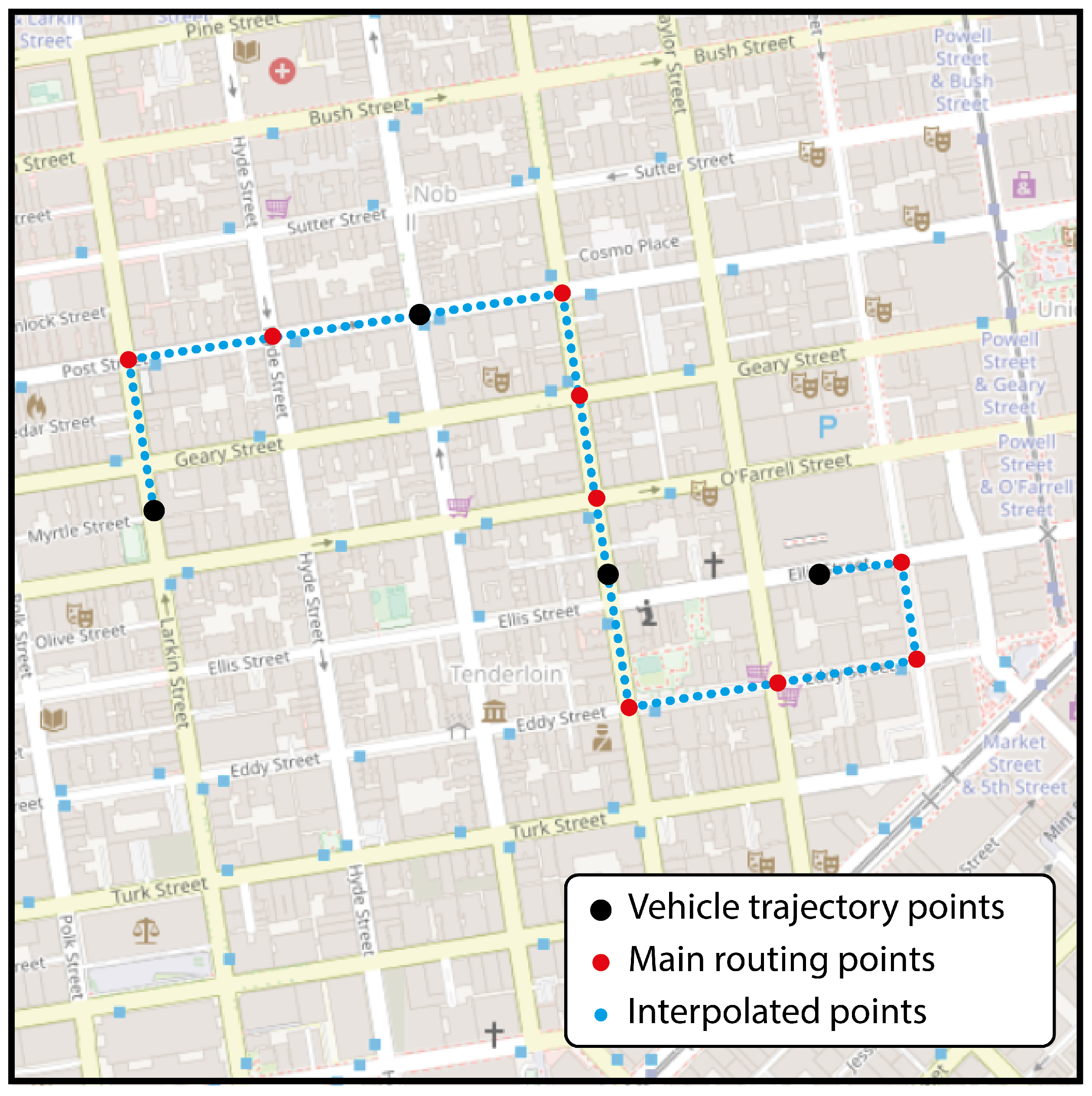
Routing and interpolation generate a denser and more continuous dataset, allowing for accurate analysis and seamless visualization of vehicle behavior along the route. This interpolated information is valuable for identifying and analyzing trends for individual vehicles, as illustrated in
Figure 2.
2.3. Step 3: Distance-Based Clustering
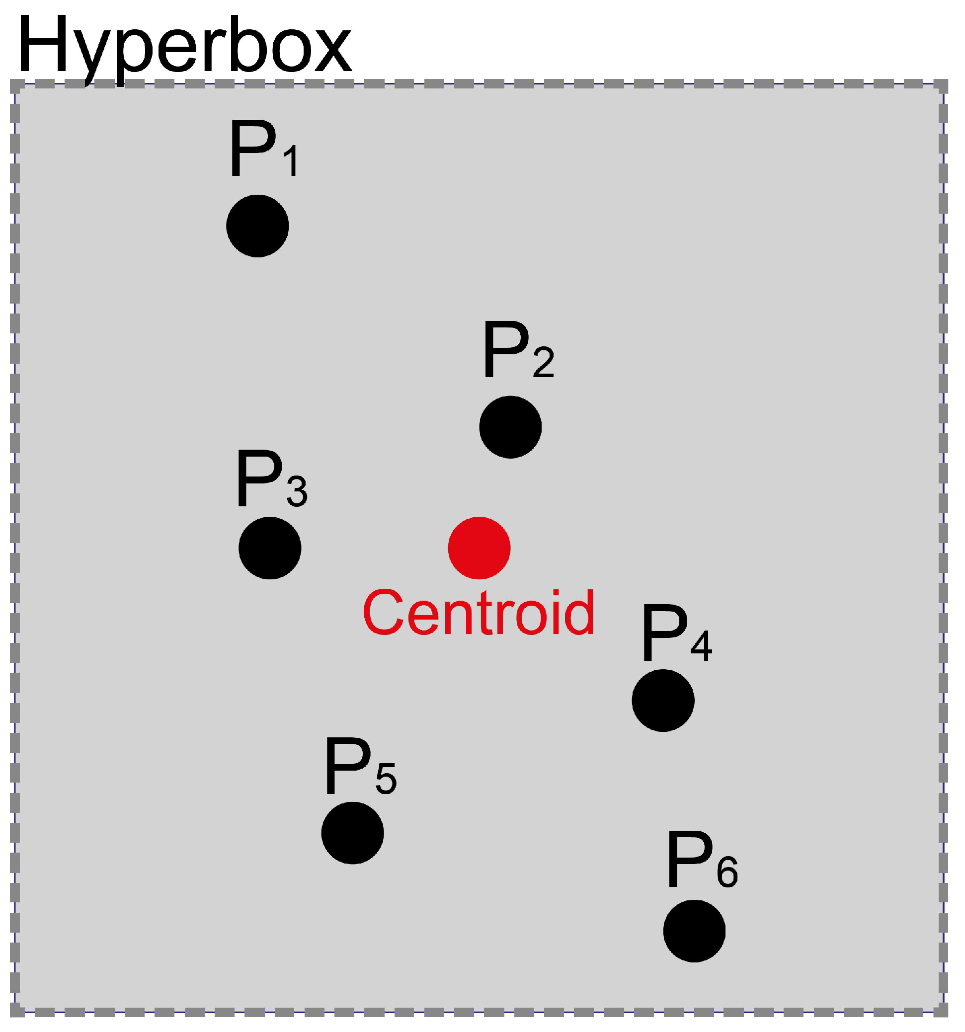
A cluster is mainly composed of a centroid, a hyperbox and linked GPS points. The centroid, which is the geographic point representing the center of the cluster, is used as a representative reference for the cluster in the analysis. The hyperbox is a rectangular structure; it is positioned according to the cluster centroid. This rectangular shape delimits an area around the centroid, which simplifies the spatial representation and determines its area of influence. The visual representation of a cluster is presented in
Figure 3.
Each GPS point processes geographic location information, vehicle identification and time of entry. Clustering is performed using similarity based on Euclidean distance, considering the latitude and longitude attributes of the GPS points. Each GPS point is analyzed by calculating the Euclidean distance with the centroids of the existing clusters. Each point is assigned to the cluster with the smallest spatial distance and within the hyperbox area.
In the case that it is not in the hyperbox area, a new cluster is created. Points assigned to a cluster cannot be reassigned to another cluster. The centroid is updated when new GPS points are integrated into a cluster, and new clusters are created if there are no nearby clusters.
To ensure that the clusters are updated and to avoid the retention of old data, a forgetting method based on the time of entry of the last GPS point is used to determine the loss of relevance as time elapses and is calculated via Equation (
1).
where
e represents the exponential function,
controls the speed of the loss in relevance and
is the difference between the time of the analyzed point and the time of the last point integrated to the cluster.
A relevance threshold of 5% is established to determine when a value is no longer relevant to the analysis. This method determines the number of GPS points that will remain in the cluster during the retention period, thus adapting the cluster to changes in traffic and avoiding the accumulation of obsolete data. Clusters that lose relevance due to the lack of new GPS points are deleted, while active clusters that continue to receive data are kept up to date.
2.4. Step 4: Classification of the Clusters According to Their Congestion Assessment
Once all the points in the temporary buffer have been assigned to a cluster, each cluster formed is evaluated by means of an indicator that analyzes the state of the traffic based on the results of the clustering at that moment. The temporary buffer can be further used to process a new data flow with its respective clustering. This step allows us to analyze and classify each cluster individually according to its congestion level, which will help us to identify problem areas and areas with better traffic flow.
Each cluster is examined individually to understand its behavior and particular characteristics; these characteristics, reflected through statistical measurements which are implicit in each road segment found within the cluster area, have been present since its initial formation and are updated each time the cluster presents changes; from the segments information, we can obtain the number of GPS points, the average speed of vehicles (unit measured in kilometers per hour, km/h) and the number of vehicles, among others.
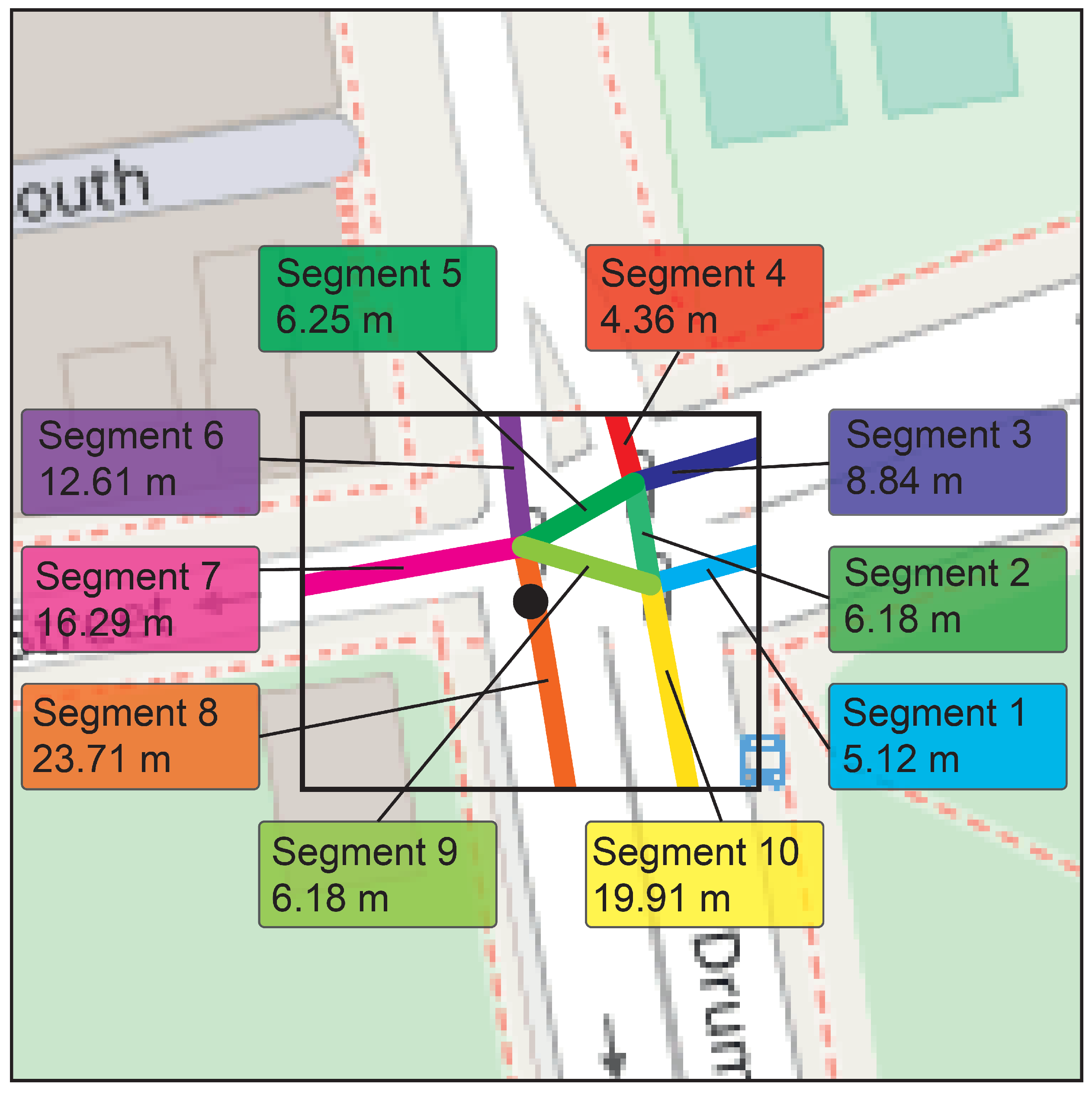
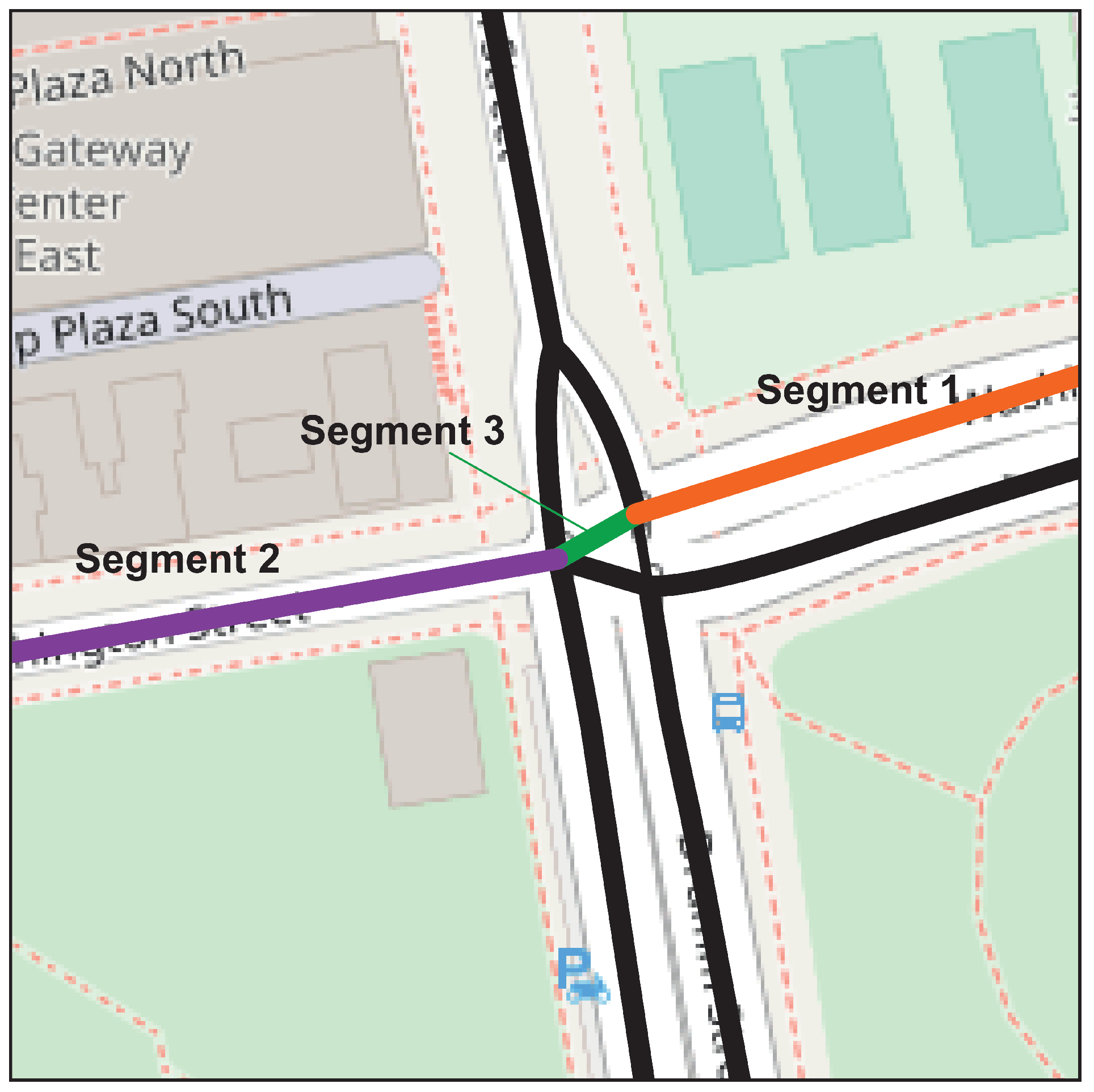
A hyperbox is spatially projected for each cluster to delimit its respective area of analysis. Map data are used to identify the roads and road segments contained within the delimited area of each cluster. A spatial clipping is applied to the roads to fit within the area defined by the hyperbox for each cluster; this allows for isolating the relevant road sections that influence each specific cluster. An example of this clipping can be seen in
Figure 4. Additionally, information associated with the geometry and metadata of each road will be used.
For the classification of the congestion status of the clusters, a Traffic Coefficient Indicator is used as a congestion indicator. The congestion indicator used indicates a value that reflects the level of congestion at a location or road [
42], quantitatively measuring congestion based on the density of vehicles and their speeds. A high value of this congestion indicator indicates significant congestion, while a low value of the congestion indicator suggests smooth traffic.
The Traffic Coefficient Indicator, used to evaluate congestion, is based on a theoretical and experimental basis in a previous article [
42]. Validation of this indicator was carried out through experimentation by subjecting the model to various conditions and scenarios. Some limitations that were observed are the dependence on the availability and accuracy of the information of the road networks; in addition, during the first execution cycles within our methodology, a decrease in the accuracy of the indicator was observed, a phenomenon that we attribute to the adaptation of the model to the specific particularities of the data in each execution.
The calculation of this congestion indicator is performed via road segments. Since a hyperbox of a cluster may comprise several segments, the congestion indicator is calculated individually for each segment. Then, a unified value is generated based on the length of the segments with at least one vehicle so that each cluster has its own value generated by the congestion indicator.
The value of the congestion indicator is calculated via the relationship between the Density Index and the Speed Index.
The Density Index represents the number of vehicles on a road segment at a specific time. It is calculated by dividing the number of vehicles observed in the area by the maximum number previously recorded on its respective road segment.
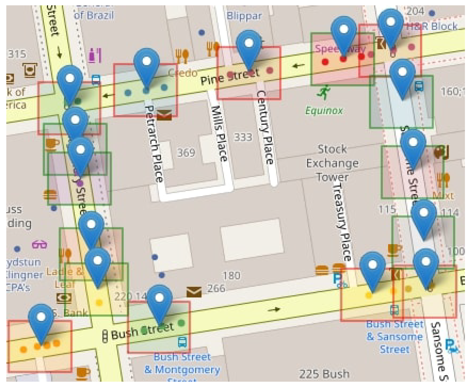
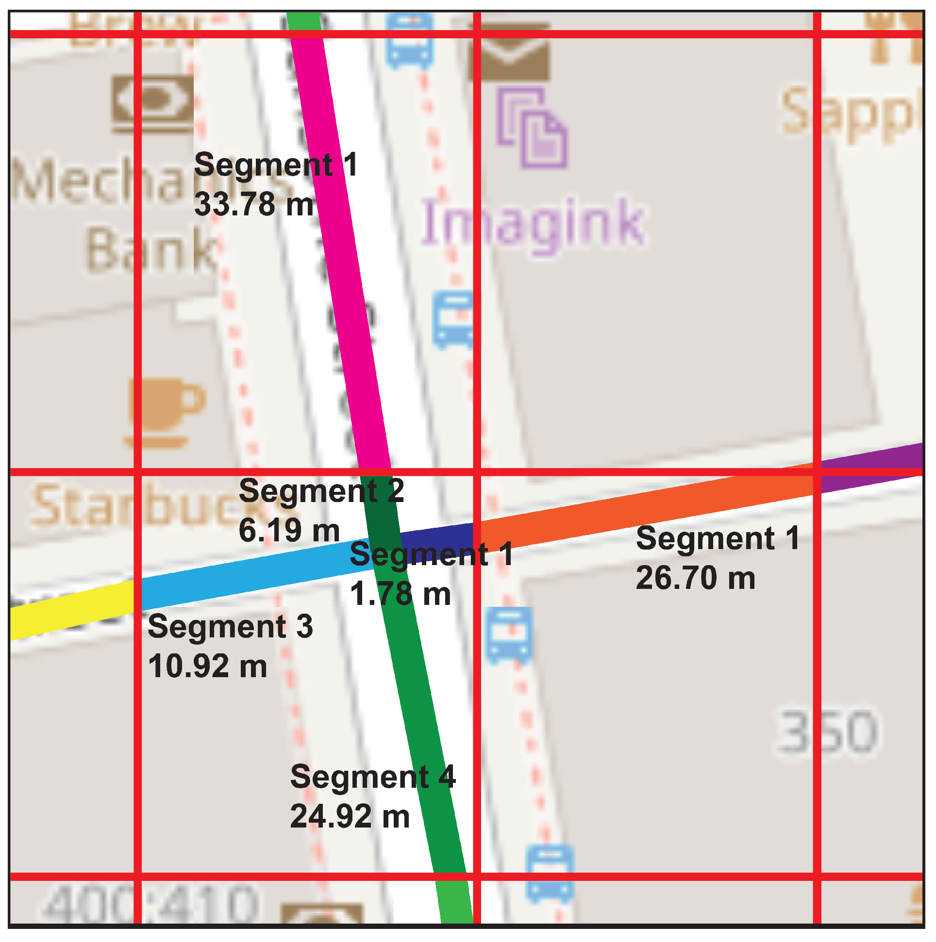
This maximum amount is based on historical data or previously conducted traffic studies. In this research, a systematic procedure for the dynamic determination of the maximum traffic density value is established. The procedure begins by identifying the road segments in the study area, as shown in
Figure 5, and calculating the traffic density of each. These densities are converted into density per unit length (D/L) values, considering the different lengths of the segments.
Then, the proportion of each segment is calculated as a function of its length with respect to the total number of segments traveled. The weighted values of density per unit length are obtained by multiplying the D/L with the proportions of each segment and adding them together to obtain a representative measure of the cluster under consideration.
The densities of all clusters in the cycle are then used and averaged to obtain an overall value for that cycle. This value is added to a historical record that is updated each cycle. With this historical value, the maximum traffic density can be estimated in a generalized manner for different road segment lengths by multiplying the historical value by the length of the road under analysis. The inclusion of multiple road segment lengths in the historical record ensures accuracy and reliability in determining the maximum traffic density, regardless of the length of the segment under analysis.
When the Density Index approaches or reaches 1, it indicates that the number of vehicles in that area is close to or has exceeded the maximum observed capacity. This suggests a high probability of congestion.
The Speed Index reflects the average speed of vehicles on analyzed roads. It is calculated by dividing the average vehicle speed by the speed limit set by local traffic regulations. These regulations are determined according to the regulations of each city, with the purpose of ensuring adequate traffic flow.
It is calculated by dividing the average speed of vehicles observed on each segment by the maximum speed allowed on the respective road segment.
When the Speed Index is close to or equal to 1, vehicles are traveling at the maximum allowable speed, indicating smooth traffic flow and low congestion. Conversely, a lower speed indicates a slower flow of traffic, which could indicate the presence of congestion.
2.5. Step 5: Results Visualization
In this study, trajectory information is examined at regular intervals, allowing for the accurate detection of changes in vehicular flow.
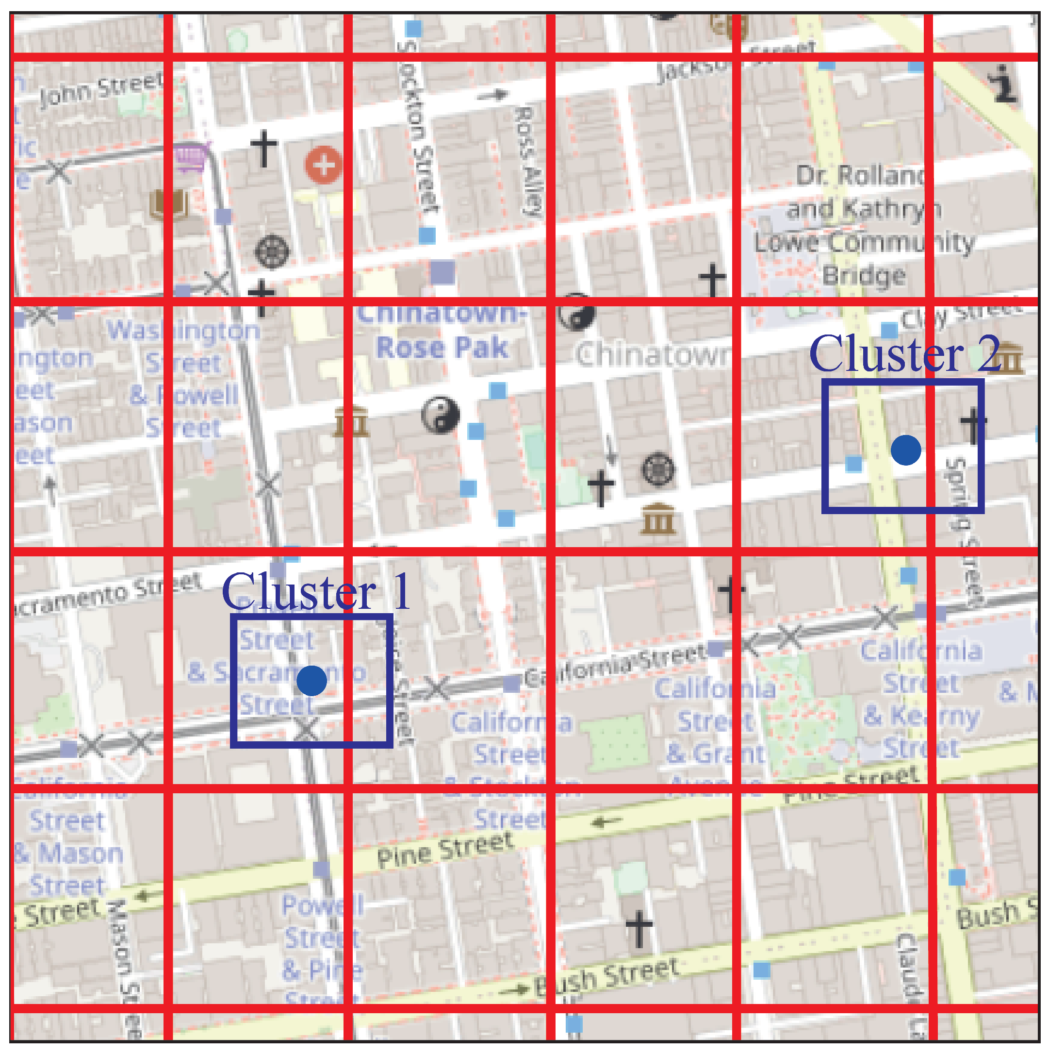
In order to provide a visual and interactive representation of the results of each cluster, an interactive map is developed that can be generated in any cycle. This map allows for dynamic and graphical analysis of the relevant information for each cluster. Each area with similar characteristics is represented with a different color on the map, as illustrated in
Figure 6.
For its applicability in traffic management systems, we propose a gradual strategy that prioritizes interoperability with existing systems. We propose the development of an interface that facilitates seamless integration, allowing for a smooth transition to implementation. In addition, we suggest a thorough evaluation of usability through pilot testing in specific urban environments, addressing challenges such as adaptation to complex traffic patterns, efficient management of large volumes of real-time data and effective interaction with traffic operators. We stress the importance of close collaboration with traffic authorities and practitioners in the field to obtain valuable feedback on the integration of the tool into everyday practices.
3. Results
3.1. Used Data
San Francisco Dataset
The data for the city of San Francisco were obtained on 2 June 2008 and cover a total of 290 trajectories followed by cabs that were equipped with GPS positioning devices.
Each record includes detailed information such as a trajectory identifier, latitude and longitude coordinates, time information, speed and direction. In this set of trajectories, an analysis of all routes recorded during the time interval from 12:30 p.m. to 13:30 p.m. was conducted. After this selection process, 2382 records were obtained, representing all 290 trajectories contained in the original dataset.
The area that represents the selected dataset is shown in
Figure 7.
3.2. Model Parameter Selection
The choice of values is focused on effective applicability in the urban environment. In this work, an analysis area of 1200 × 800 square meters selected from a region of the city with a diverse vehicular flow is delimited. The hyperboxes represent approximately 3% of the analysis area and have a size of about 35 × 25 m; their proportion with respect to the analysis area suggests an adaptation to the scale of the environment. The hyperboxes capture patterns mainly on streets and intersections without sacrificing the granularity of the analysis. The analysis cycles have a duration of 1 min each, chosen to perform frequent evaluations and capture traffic dynamics in near real time. Euclidean distance is used as the similarity measure which is common in clustering problems and suggests a standard approach for evaluating spatial relationships. The forgetting parameter was set to 0.068 and 0.05, to consider relevant data up to 45 and 60 s, respectively. These values reflect a careful decision to balance the consideration of recent and past data, influencing the model’s ability to adapt to changes in traffic flow. Clusters with low activity are updated every 30 s, and old clusters are removed if they have stopped receiving new points after 2 min.
3.3. Model Testing
To demonstrate the advantages of the dynamic clustering methodology compared to the congestion indicator applied to static cells, a model test was performed. The main objective of this test was to analyze how the methodology deals with the dynamics of traffic data and vehicular flow in a road network, identifying situations in which it is superior.
A dataset representative of the city of San Francisco was used, comprising six run cycles in a 100 × 100 m area. A cluster of data from this test was randomly selected for comparative analysis.
The dynamic clustering methodology excels in its ability to adapt to variations in data distribution.
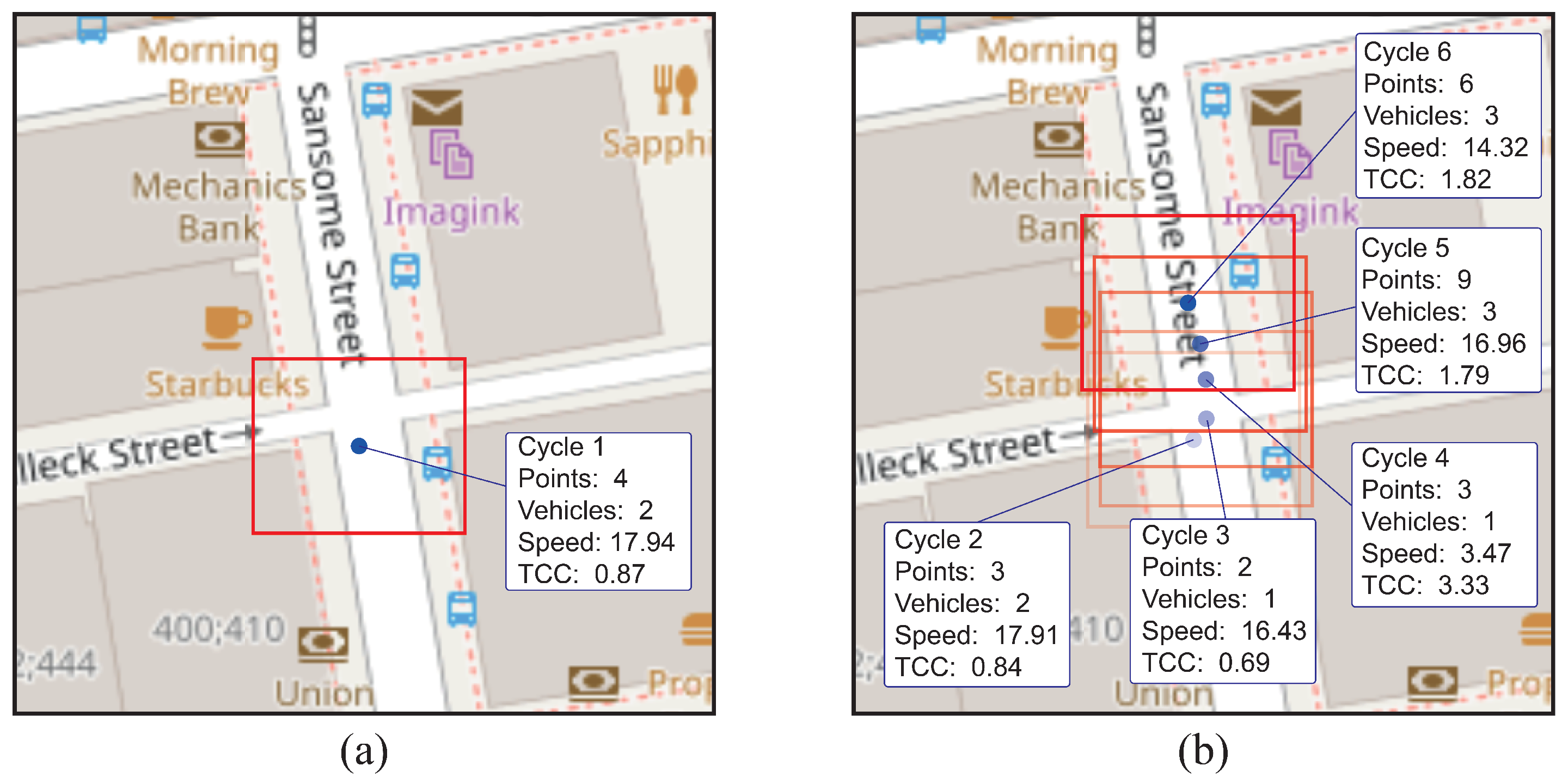
Figure 8a shows how the hyperbox was flexibly and accurately adjusted to encompass road segments, effectively capturing variations in density and shape of the clusters as the data evolved, as can be seen in
Figure 8b. In addition, this methodology demonstrated a clear advantage in the selection of road segments subject to variations in vehicular flow and traffic density.
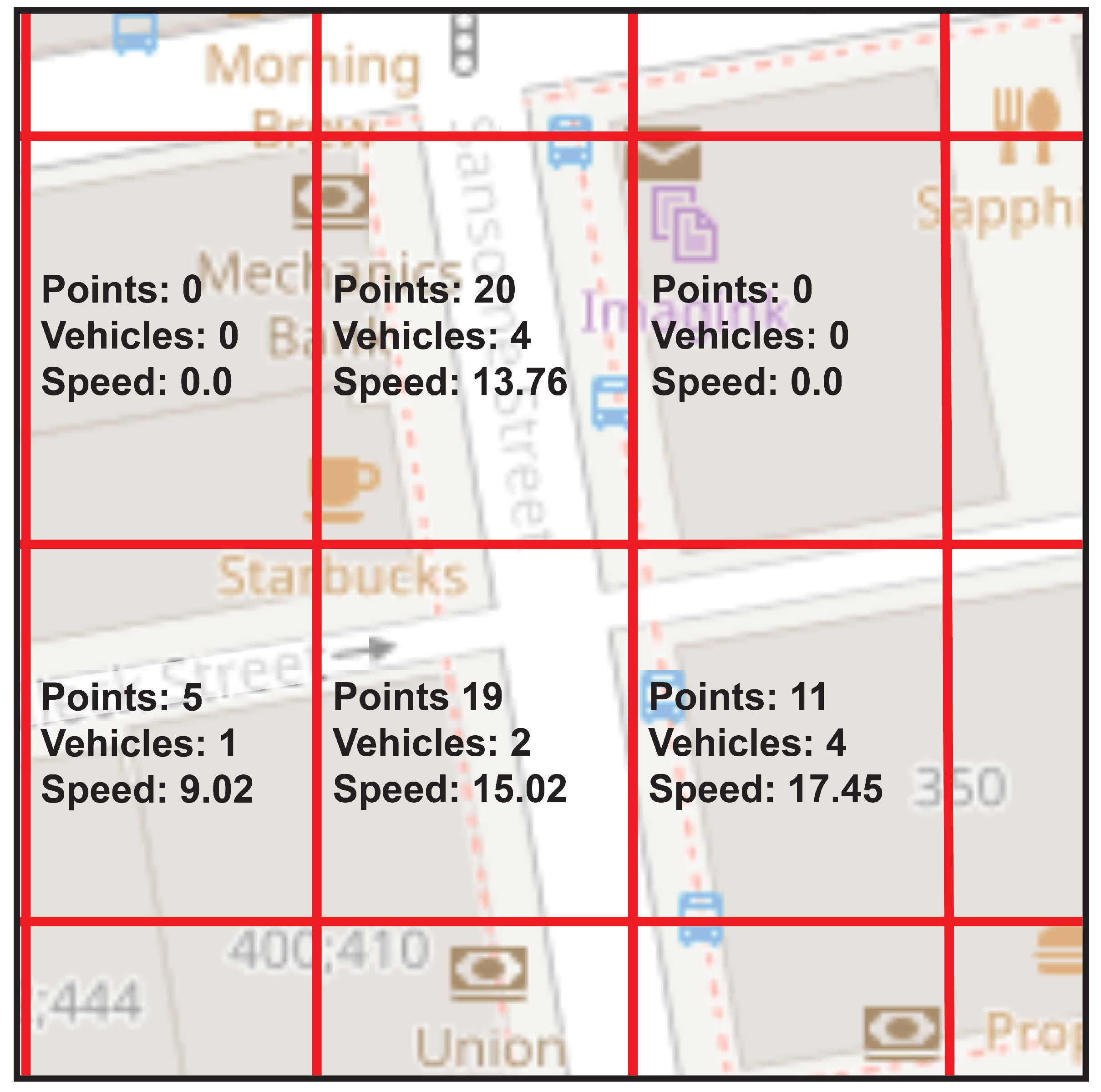
In contrast, the congestion indicator applied to static cells uses a fixed grid, which is seen in
Figure 9. This limits its adaptability and can compromise the quality of the results by not adjusting to changing patterns of vehicle trajectories. Not being able to adapt to how data are clustered over time makes it unsuitable for identifying congestion events in dynamic traffic scenarios.
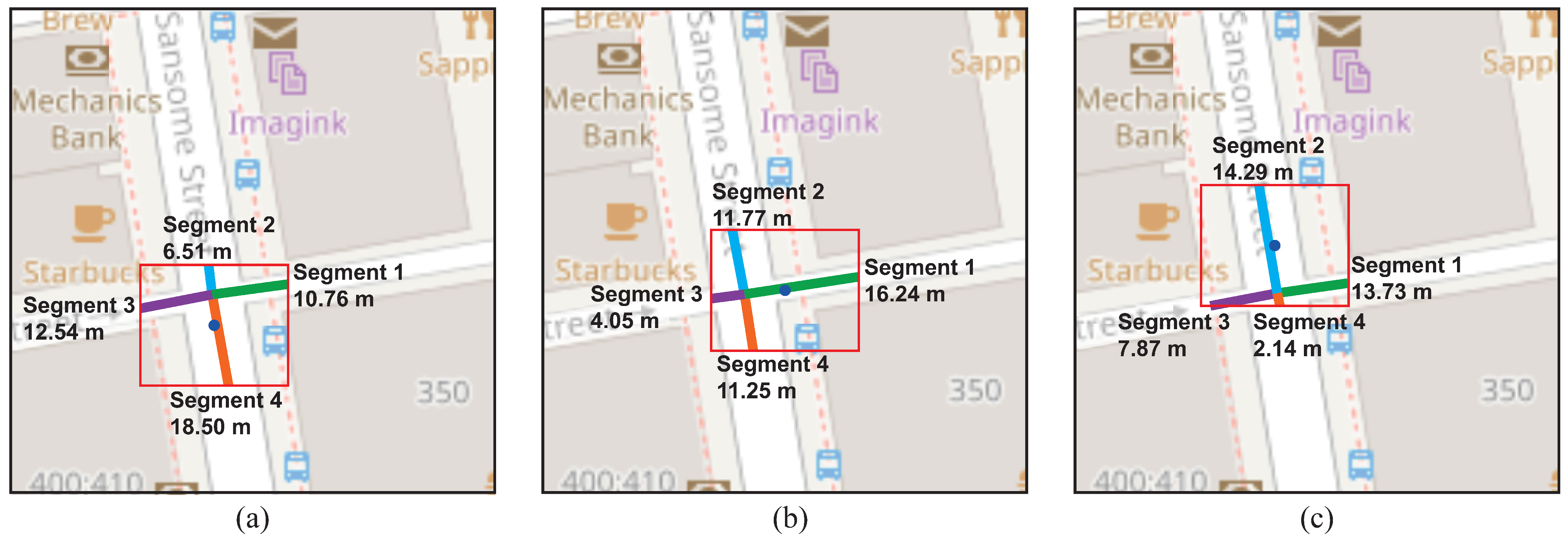
The dynamic clustering methodology also demonstrates a significant advantage in terms of adaptability to data dynamics. In
Figure 10, its ability to select road segments in cycles 1, 3 and 5 is seen, allowing it to adjust to fluctuations and changes in the data distribution. This methodology can modify the position of the centroids and hyperbox as needed, making it a suitable choice for selecting road segments subject to variations in vehicular flow.
In contrast, the congestion indicator applied to static cells faces difficulties when dealing with these dynamics due to its fixed grid. In real scenarios, where roads experience fluctuations in the number of vehicles throughout the day, the congestion indicator applied to static cells may select incorrect road segments for each cell, as seen in
Figure 11. This can lead to an incorrect representation of traffic at different times of the day.
A highlight of the dynamic clustering methodology is its ability to incorporate more recent vehicle locations in real time, resulting in an automatic update of the cluster centroids. This ensures that newer locations have a greater impact on defining real-time congestion, while older locations become less and less relevant. This is crucial, as a vehicle can cross multiple cells in a single trip. The dynamic clustering methodology ensures an accurate and sensitive assessment of congestion, adapting to the changing mobility of vehicles on urban roads.
3.4. Obtained Results
In this research, the results of the dynamic clustering methodology were compared with the results of the congestion indicator applied to static cells to analyze vehicular flow using the Traffic Coefficient Indicator to measure congestion, as shown in
Figure 12.
In the dynamic clustering methodology, the vehicle data were grouped into similar patterns and the location of the cluster determined the area of comparison, while in the static cells, the area was divided into uniform cells. Both cases are evaluated using the congestion indicator.
A tolerance was applied to the indicator values in dynamic clusters to account for the natural variability of the data and to avoid the misidentification of possible congestion states. The tolerance determines how great a margin of error is allowed when adjusting the congestion indicator, directly influencing the number of matches observed in the congestion classification. The congested classification results were then compared between cells and clusters, recording valid matches when at least one cell matched the same congestion classification as the cluster.
To determine if the cluster classification was performed correctly, the results of the model using confusion matrices are compared to the results from the city of San Francisco. The following confusion matrices present a representation of the capabilities of the dynamic cluster classification model relative to the static grid model. The values reflect the number of accurate and erroneous predictions in the congested and non-congested categories. These results provide detailed insight into how the model interprets and predicts the congestion state in the clusters, which is essential for evaluating its performance in real traffic situations.
The confusion matrix for the city of San Francisco, with a forgetting value of 45 s and no tolerance, is presented in
Table 1. In the congestion cases, 6433 were correctly classified, and of the non-congested cases, 10,932 were correctly classified. However, 1273 errors were made in misclassifying non-congested situations as congestion, and 6307 errors were made in classifying congested situations as non-congested.
The confusion matrix for the city of San Francisco, with a forgetting value of 45 s and a tolerance of 0.2, is presented in
Table 2. In the case of congested clusters, 6881 cases were correctly classified as congestion, and in the case of non-congested clusters, 12,387 cases were correctly classified as non-congested. However, 825 errors were made in misclassifying non-congested situations as congestion, and 4852 errors were made in classifying congested situations as non-congested.
The confusion matrix for the city of San Francisco, with a forgetting value of 60 s and no tolerance, is presented in
Table 3. For congested clusters, 6708 cases were correctly classified as congestion, and for non-congested clusters, 10,776 cases were correctly classified as non-congested. However, 1390 errors were made in misclassifying non-congested situations as congestion, and 6293 errors were made in classifying congested situations as non-congested.
The confusion matrix for the city of San Francisco, with a forgetting value of 60 s and a tolerance of 0.2, is presented in
Table 4. For congested clusters, 7177 cases were correctly classified as congestion, and for non-congested clusters, 12,232 cases were correctly classified as non-congested. However, 921 errors were made in misclassifying non-congested situations as congestion, and 4837 errors were made in classifying congested situations as non-congested.
These results indicate that, compared to previous parameterizations with a forgetting value of 45 s, the model presents slightly better quantities in identifying congested situations. When evaluating the true positive rate, that is, the ability to correctly identify the congested state of traffic, the clusters obtained a high number of matches compared to the congested grid cells in the city of San Francisco.
4. Discussion
In this section, we examine the results obtained from the comparison between the dynamic clustering methodology and the congestion indicator applied to static cells in the city of San Francisco. The evaluation metric is represented by the precision rates which provide an in-depth understanding of the performance of both results.
The precision is obtained using Equation (
2):
where
represents the number of true positives, i.e., cases that the model correctly classifies as congested, and
represents the number of false positives, i.e., cases that the model incorrectly classifies as congested when they are actually non-congested.
In this research, a detailed analysis of the congested cluster classification was carried out in the traffic congestion study, as this classification plays a central role in urban traffic management and in improving mobility in cities. Congested clusters represent problematic traffic scenarios that can have a significant impact on urban mobility and citizens’ quality of life. Accurately identifying and classifying these situations is essential for making informed traffic management decisions and applying effective congestion relief strategies.
The precision results for the clusters categorized as congested are displayed in
Table 5. The results table provides important insight into the precision of the comparison between the congested clusters of the dynamic cluster method and the congested cells of the static grid method in identifying traffic congestion. Two key parameters, forgetting and tolerance, have been evaluated to understand their impact on the precision of the results.
The methodology for identifying congested areas is characterized by the variation in forgetting values between 45 and 60 s, evidencing an inverse relationship between this parameter and precision. In the choice of the forgetting value, it is important to balance capturing recent dynamics and the relevance of past events. However, exploring tolerance, especially at levels like 0.2, suggests that allowing a margin of error can improve accuracy.
The identification of optimal combinations, such as a 45 s forgetting with a tolerance of 0.2, highlights the existence of suitable parameter combinations for effective detection based on the accuracy rates of congested zones in dynamic environments.
The results highlight the crucial influence of the parameters forgetfulness and tolerance on the precision of traffic congestion prediction. It is clear that the appropriate choice of these values is a determining factor in achieving optimal precision in the classification of congestion situations. The configuration of these parameters must be precisely aligned with the specific application requirements and prediction objectives.
However, it is important to note that this improvement in precision by reducing the forgetting value and increasing the tolerance can also have implications for other aspects of the analysis. A lower forgetting value means that a narrower time window is being considered, which may result in the loss of relevant information in the long term. In addition, a higher tolerance implies a wider margin of error, which could allow for the inclusion of noisy data that affects precision in certain situations.
Therefore, finding the right balance between these parameters is a key challenge in the practical application of these methods. The choice of optimal values for forgetting and tolerance will depend on the specific needs of the congestion prediction task and the importance of maintaining precision compared to other factors, such as the retention of historical information and management of noise in the data.
In analyzing these results, it is essential to highlight the efficiency of the clustering algorithm in detecting vehicle congestion compared to the method based on static cells in fixed regions. The high levels of precision strengthen the algorithm’s ability to identify congestion patterns in the data and anticipate future situations.
Furthermore, looking at the comparison made in the model testing, it is evident that the lack of adaptability of the congestion indicator applied to static cells to adjust to the evolution of the data and changes in the distribution of clusters may affect the quality of the results. If congestion data and traffic flows are not properly identified due to this lack of adaptability, the detection of congested areas may lack reliability.
On the other hand, a dynamic clustering methodology that accounts for variations in data flows and adapts to changes in cluster distribution provides an accurate representation of traffic dynamics. As shown in
Table 6, statistical data for a specific cluster indicate that the speeds of cycle 4, although belonging to the same cluster, have undergone unusual changes. This is due to the fact that the cluster incorporates information from different registered vehicles, which allows for better adaptation to traffic evolution.
By continuously recalibrating the centroid position and adjusting the hyperbox based on evolving data, this methodology effectively captures variations in densities and shapes of the road segments. This can be seen in
Table 7, which shows the information used to analyze the cycle 5 road segments. In this table, it can be seen that out of four segments identified, only three of them have recorded vehicles. As each segment is analyzed independently, it is possible for a vehicle traveling through several segments to be counted as a single vehicle in the context of another segment. The visual representation for this table is associated with
Figure 10c. This allows for groupings to be made based on up-to-date data and realistic evaluations.
5. Conclusions
The obtained results highlight the effectiveness of the dynamic clustering methodology compared to the static cell-based method for classifying congestion conditions. By allowing dynamic clustering of vehicle trajectory data and performing specific analysis for each cluster, this methodology facilitates early and accurate detection of congested traffic problem areas.
The application of dynamic clustering methods presents itself as a highly promising strategy. These methods have the ability to adapt to constant changes in urban traffic, capturing constantly evolving mobility patterns. The relevance of the forgetting factor lies in its ability to keep the clusters up to date, considering both recent and old locations. This ensures that the clusters accurately reflect current traffic dynamics, allowing emerging congestion to be identified early.
Carefully tuning the forgetting and tolerance parameters is critical for obtaining accurate results in the comparison between dynamic cluster and static grid methods in traffic congestion prediction. These findings are essential for improving the effectiveness of classification models in traffic management applications.
The methodology based on dynamic clustering stands out for its adaptability to changes in traffic, providing a complete and up-to-date view of vehicular behavior in urban areas. These results support the effectiveness of clusters as a valuable tool for improving traffic management and reducing congestion problems in cities.
Our study recognizes several important limitations. The generalization of the findings to different urban settings highlights the need to validate the methodology in various cities and urban regions. The tests were focused on static comparisons. It is important to expand the comparisons to dynamic approaches for a more complete evaluation of key challenges.
In addition, performance could be slower than expected due to the microbatch implementation, so it is necessary to investigate and optimize the efficiency of the system, and the congestion indicator, although dynamic, may present initial errors and require stabilization. This is a process which can be improved.
Performance needs to be addressed in real time, optimizing the microbatch implementation or exploring different approaches that allow for a faster response, linked to an improvement in the model with a focus on efficiency and the calculation of the congestion indicator dynamically.
As for future research, it is essential to explore in depth the possible reasons behind the observed decrease in precision in the congested classification. In addition, it is proposed to conduct experiments in larger areas, under extreme congestion conditions and in highly complex traffic scenarios. These experiments will provide additional insight into the limits and robustness of the proposed methodology.


 ,
, 


