Article

Design and Control of Hydraulic Power Take-Off System for an Array of Point Absorber Wave Energy Converters

1
Institute of Marine Science and Technology, Shandong University, Qingdao 266237, China
2
Key Laboratory of High-Efficiency and Clean Mechanical Manufacture of Ministry of Education, National Demonstration Center for Experimental Mechanical Engineering Education, School of Mechanical Engineering, Shandong University, Jinan 250061, China
*
Authors to whom correspondence should be addressed.
Sustainability 2023, 15(22), 16092; https://doi.org/10.3390/su152216092
Submission received: 4 October 2023 / Revised: 9 November 2023 / Accepted: 17 November 2023 / Published: 19 November 2023
(This article belongs to the Topic Wind, Wave and Tidal Energy Technologies in China)

Abstract

:
The development of wave energy converter (WEC) arrays is an effective way to reduce the cost of levelized energy and facilitate the commercialization of WECs. This study proposes a hydraulic power take-off (PTO) system for an array of point absorber wave energy converters (PA-WECs) and designs a control system using a novel algorithm called the improved simplified universal intelligent PID (ISUIPID) controller and the adaptive matching controller including an improved artificial gorilla troops optimizer (IGTO) to improve and stabilize the output power of PA-WEC arrays. Simulations under varying irregular wave states have been carried out to verify the validity of the mathematical model and the control system. The results show that the designed IGTO has faster convergence speed and better convergence accuracy in solving the optimal linear damping coefficient of the generator, and the proposed ISUIPID controller provides superior performance in tracking the speed of the hydraulic motor under the changing sea states. In addition, the capture power and output power of the array of PA-WECs are improved and the electrical energy can be output stably under the designed control system. The array of PA-WECs with the proposed control system will become an independent, stable, efficient, and sustainable power supply system.

1. Introduction

Developing and utilizing clean, renewable, and sustainable marine energy sources is a key way to address environmental pollution and the energy crisis. Wave energy is one of the most promising marine renewable energy sources, characterized by high energy density and sustainable power supply compared to the well-established solar and wind energy [1,2]. A wide variety of wave energy converters (WECs) have been designed to utilize wave energy, such as oscillating water column WECs, overtopping WECs, and PA-WECs [3,4,5,6]. Among them, PA-WECs have developed rapidly in recent years due to their high conversion efficiency, flexible structure, and adaptability [7,8]. However, the high levelized cost of energy hinders the commercial development of WECs [9,10]. The development of arrays of WECs has been considered as an effective way to significantly reduce cost, while also offering the advantage of improving reliability [11,12].
A lot of recent research around the hydrodynamic characteristics and layout optimization of arrays of WECs has been carried out. Andres et al. found that the distance between WECs, array layout, number of WECs, and wave directionality had an impact on the energy capture characteristics of WEC arrays [13]. Lyu et al. adopted genetic algorithms to explore the optimal dimension for each wave energy converter in an array of WECs. The study demonstrated that for WEC arrays with an optimal control or a derivative control, optimizing the buoys dimensions simultaneously with the array layout had a positive effect on the energy harvesting performance of WEC arrays [14]. Faedo et al. proposed a multi-input, multi-output parameterization strategy based on a system-theoretic interpretation of moments, which can accurately represent the input–output dynamics of arrays of WECs [15]. And the mathematical correlation between the proposed parameterization strategy and wave excitation force estimation strategies was used to provide low-order models that provided the same degree of wave excitation force estimation accuracy as the currently used parameterization methods [15]. To maximize the harvested energy from the array of WECs, Zou et al. presented a collective control and a surrogate model replacing the hydrodynamic model to control gain optimization, and the effectiveness of the proposed control strategy and surrogate model were verified via simulations [16]. Murai et al. provided a controlled force optimization method for PA-WEC arrays considering factors such as diffraction hydrodynamic interactions, radiation hydrodynamic interactions, wave incidence angles, and array layouts. Numerical analysis showed that power generation efficiencies increased by 15% and 5%, respectively, when the array layout and control force parameters were optimized [17].
By summarizing the previous work, it can be found that the layout optimization and theoretical optimal control strategy of WEC arrays have been investigated intensively; however, the design and control of the hydraulic PTO system for arrays of WECs are rarely studied. The PTO system has a significant impact on the efficiency and stability of WECs. And the hydraulic PTO is considered the most promising PTO system for WECs because of its higher efficiency and excellent controllability [18]. Do et al. built the mathematical model of hydraulic components of a multi-point-absorber wave energy converter and verified that the pressure fluctuation was reduced by adopting the high-pressure accumulator and multi-point absorber [19]. Gaspar et al. studied the speed control strategy of the electric-driven hybrid hydraulic wave energy conversion system, designed a fuzzy controller to adjust the motor displacement to control the pipeline pressure and a PI controller to adjust the motor load to control the motor speed for the double-cone oscillating float system, and carried out numerical simulations under different sea conditions [20]. Fan et al. studied the open-loop hydraulic PTO system and designed a fuzzy controller to control the displacement of variable motors based on the motor torque deviation signal so that the output torque and output power of the motor were close to the target value [21]. Geng et al. proposed a novel power regulation module comprising a throttle valve and a pressure compensation valve in the hydraulic PTO system. The results demonstrated that the power regulation module stabilized the hydraulic motor speed and output power [22]. Chen et al. designed a PID controller to stabilize the rotational speed of the hydraulic PTO system and verified the effectiveness of the controller using experiments [23].
The focus of this paper is to improve and stabilize the output power of the hydraulic PTO system for arrays of PA-WECs. The main contributions of this paper are as follows: (1) a controllable hydraulic PTO system for arrays of PA-WECs is proposed; (2) a novel intelligent control algorithm called the ISUIPID with ease of design and implementation is designed to improve the stability of the output power of WEC arrays under irregular wave states; (3) an adaptive matching controller including the IGTO algorithm is designed to enhance the capture power and output power of WEC arrays.
The remainder of this paper is organized as follows: Section 2 describes the hydraulic PTO system. The mathematical modeling is provided in Section 3. Section 4 discusses the control system in detail. Simulation results and analysis are shown in Section 5. Finally, some important conclusions are given in Section 6.

2. System Overview

The schematic of an example of the proposed system is shown in Figure 1. The number of buoys can be multiple, using three as an example in this paper. In this paper, the array of PA-WECs involves three cylindrical buoys, three hydraulic cylinders, three hydraulic check valve groups, a hydraulic accumulator, a relief valve, a variable displacement hydraulic motor, and a generator. In this system, each buoy is connected to the two-way hydraulic piston of its corresponding anchoring hydraulic cylinder separately. Under the excitation of the waves, the buoys drive the two-way hydraulic pistons to move up and down to absorb the wave energy and convert it into hydraulic energy. Using the hydraulic check valve groups, the hydraulic cylinders always draw low-pressure oil from the hydraulic tank, and the high-pressure hydraulic oil is always injected into the accumulator, regardless of whether the two-way hydraulic pistons move up or down. Here, the accumulator acts as a buffer to absorb the pressure fluctuation and reduce the pressure shock. An outlet of the accumulator is connected to the inlet of the variable displacement hydraulic motor. The high-pressure hydraulic oil output by the accumulator drives the hydraulic motor and the generator connected in tandem with it to rotate and generate electricity at the same speed. The other outlet of the accumulator is connected to the hydraulic oil tank through the relief valve. The relief valve is a safety valve that limits the system pressure. When the system pressure is higher than the set value, the relief valve is opened, and the high-pressure hydraulic oil flows into the hydraulic oil tank to relieve the system pressure. And a control system is designed to adjust the displacement of the variable hydraulic motor (Vm), and the linear damping coefficient of the generator (Cg) improves and stabilizes the output power.

3. Mathematical Modeling

3.1. The Hydrodynamics of Array Buoys

In this paper, the array buoys are semi-submerged cylinders and are assumed to move only in heave. The hydrodynamic time-domain equation of the heave motion for an array of WECs can be expressed as:
M Z ¨ ( t ) = F e x ( t ) + F r ( t ) + F s ( t ) + F v ( t ) + F P T O ( t )
where Z ¨ ( t ) is the heave acceleration vector consisting of the heave acceleration of each buoy. F e x ( t ) , F r ( t ) , F s ( t ) , and F v ( t ) are the excitation force vector, radiation force vector, hydrostatic buoyancy force vector, and viscous damping force vector, respectively, which are composed of the excitation force f e x i t , radiation force f r i t , hydrostatic buoyancy force f s i t , and viscous damping force f v i t of each buoy. F P T O ( t ) is the force vector consisting of the force f P T O i t applied to each buoy using the PTO system. The mass matric M of the array buoys is written as follows:
M = d i a g m 11 , m 22 , , m i i , , m N N
where m i i is the mass of the i-th buoy, and N is the number of buoys in the array of WECs.
The excitation force f e x i t of the i-th buoy can be related to the incident wave field spectrum S w through the relations [24]:
f e x i t = j = 1 N w f e i w 2 S w w cos k j x w j t + θ j i + θ r
where N w is the number of waves in the irregular wave, f e i w is the excitation force of the i-th buoy in the frequency domain, which is from the frequency domain hydrodynamic analysis, and w is the constant difference between successive frequencies. k j , w j , θ j i , and θ r represent the wave number, wave frequency, phase angle between wave elevation and wave excitation force, and random phase angle for the j-th wave, respectively.
In this paper, the JONSWAP spectrum is applied, which is defined as follows [24]:
S w = 155 H s 2 T e 4 w 5 exp 944 T e 4 w 4 3.3 ε ε = exp 0.191 w T e 1 2 0.5 σ 2 σ = 0.07   f o r   w 5.24 T e σ = 0.09   f o r   w > 5.24 T e
where H s , T e , ε , and σ denote the significant wave height, the energy period, the energy scale, and the peak shape factor, respectively.
The hydrostatic buoyancy force f s i t and the radiation force f r i t take the following forms due to the buoy’s oscillation in the otherwise calm water:
f s i t = π ρ g a i 2 z i t
f r i t = m i l z ¨ i t l = 1 N t K r i l t τ z ˙ i τ d τ
where g and ρ are the gravity acceleration and the water density, respectively; and a i , z i t , and z ˙ i t are the radius, heave displacement, and heave velocity of the i-th buoy, respectively. m i l is the added-mass coefficient at the infinite frequency of the i-th buoy. The radiation impulse response function K r i l ( t ) is given as follows [25]:
K r i l t = 2 π 0 B i l ω cos ω t d ω
where B i l ω represents the radiation damping coefficient of the i-th buoy influenced by the l-th buoy at angular frequency ω .
The viscous damping force f v i t of the i-th buoy can be seen as a drag force in Morison’s equation [26]:
f v i t = 1 2 ρ C d i A d i z ˙ i t z ˙ i t
where C d i and A d i represent the drag coefficient and characteristic area of the i-th buoy respectively.
Since the determination of drag force coefficients is difficult and easy to introduce uncertainty in the model [26], and accurate modeling is not the focus of this study, the drag coefficient is taken as 0 in this paper, i.e., the effect of nonlinear viscous forces is not considered.

3.2. The Hydraulic PTO System Modeling

In this system, the relative displacement of the hydraulic piston to the hydraulic cylinder is equal to the displacement of the buoy, and it is assumed that the check valves are ideal with no pressure or flow loss.
The flow rate Q i of the accumulator inlet is calculated as follows:
Q i = i = 1 N S i z ˙ i t
where S i is the effective area of the i-th hydraulic piston.
The force f P T O i of the PTO system acting on the i-th buoy is shown as follows:
f P T O i = P s S i
where P s is the system pressure.
The time average capture power P c i of the i-th buoy can be calculated as follows:
P c i = 1 t e 0 t e f P T O i z ˙ i t d t
where t e is the calculation end time.
The function of the hydraulic accumulator is to absorb the pulsations generated by the wave energy fluctuation. The process of the hydraulic accumulator absorbing and releasing wave power is assumed as the adiabatic change process. The pressure–volume transient variation equation of the gas in the hydraulic accumulator is shown as follows:
P s V 0 V 1.4 = P 0 V 0 1.4
where P 0 and V 0 are the initial gas pressure and gas volume respectively. The change in the gas volume V is given as follows:
V = Q i Q o d t
where Q o is the outlet flow of the hydraulic accumulator, which is the inlet flow of the hydraulic motor.
The speed n m , torque T m , and output power P m of the hydraulic motor are expressed as follows:
n m = Q o η V V m
T m = P s V m η m 2 π
P m = P s Q o η V η m
where V m , η V , and η m represent the displacement, volumetric efficiency, and mechanical efficiency of the hydraulic motor respectively.
The dynamic model of the hydraulic motor and generator rotor is established as follows:
J m + J g ω ˙ m = T m C g n g
ω m = 2 π n m
n m = n g
where J m is the rotational inertia of the hydraulic motor, J g is the rotational inertia of the generator rotor, ω m is the angular speed of the hydraulic motor, and C g and n g are the linear damping coefficient and speed of the generator respectively.

4. Control System Design

The basic architecture of the control system for the array of WECs is shown in Figure 2. The input to the control system is the ideal speed of the hydraulic motor, which in this system is equal to the rated speed of the hydraulic motor and the generator to make the generator and the hydraulic motor operate at optimal efficiency. In order to improve the efficiency and stability of power generation, a speed controller is designed to ensure constant speed operation of the hydraulic motor by adjusting its displacement, and an adaptive matching controller is designed to improve the output power of arrays of WECs by adjusting the linear damping coefficient of the generator.

4.1. The Speed Controller

Because of the high randomness and irregular fluctuations of waves in real sea states, a satisfied control effect is very difficult to obtain using a conventional PID controller. So the ISUIPID controller with the advantages of simple design and intelligence is designed to keep the hydraulic motor speed to meet the ideal speed and enhance the stability and immunity of the control system under irregular incident waves. To verify the superiority of the proposed ISUIPID, the control effects of the PID controller and the fuzzy PID controller are also shown.

4.1.1. The ISUIPID Controller

The ISUIPID controller is the one proposed for the hydraulic PTO system of the array of WECs to achieve the ideal hydraulic motor speed under varying sea states to overcome the shortcomings of traditional and intelligent algorithms. Most modern intelligent algorithms are complex and require periodic updating of parameters throughout the operation. In addition, the adjustment of parameters is very complex and requires rich experience. Therefore, there is a lot of research trying to simplify and improve the controller. Combining simplification with intelligence is challenging because increasing the intelligence of a controller inevitably leads to an increase in system complexity, which can only be achieved by making the system intelligent or simple [27].
In order to achieve intelligence and simplicity in the control system, a new technique known as SUIPID controller has been proposed [28]. The SUIPID controllers use simple design and adaptive techniques that combine the advantages of traditional methods and intelligent algorithms. The design of the controller is divided into two steps: one is a simple adaptive PID controller and the other is the application of the multiple degrees of freedom (MDOF) concept. The MDOF utilizes two controllers with different gains operating simultaneously in the wide range of errors and in the fine-tuning region; the first controller handles large errors for fast error correction, while the other handles small errors for fine-tuning [27,28]. The final output (O/P) composed of the outputs of two controllers is as follows [28]:
O / P = O / P 1 · e + O / P 2 · 1 e
where e is the normalized error. When the error is large, ( 1 e ) is relatively small, and O / P 1 plays the main role. On the contrary, when the error is small, ( 1 e ) is relatively large, and O / P 2 plays the main role. So O / P 1 is the output of the first controller dealing with the significant error, and O / P 2 is the output of the second controller that deals with the fine-tuning error.
Figure 3 shows the SUIPID control architecture. Two adaptive weights, error (e) and (1 − e), were added to the two controllers to obtain an appropriate response. As shown in Figure 4, these two controllers can be designed as an intelligent PID (IPID) controller with the following adaptive parameters:
K p = e K i = e d t K d = d e d t
The final output (O/P) of the SUIPID controller is as follows:
O / P = O / P 1 · e + O / P 2 · 1 e
O / P 1 = K · ( e e + e d t e d t + d e d t d e d t )
O / P 2 = 1 K · ( e e + e d t e d t + d e d t d e d t )
From Equations (23) and (24), it can be seen that O / P 1 and O / P 2 are the products of the output of the IPID and the controller gains K and 1 K , respectively. Although this can result in only one controller parameter, it also constrains the controller’s ability to handle the significant error and the fine-tuning error, i.e., the controller’s ability to handle the significant error and the fine-tuning error is approximately reciprocal. Therefore, the ISUIPID controller was proposed, which does not limit the control gain of the two IPID controllers to a reciprocal relationship. The output of the ISUIPID controller ( O / I P ) can be calculated as follows:
O / I P = O / I P 1 · e + K 2 · O / I P 2 · 1 e
O / I P 1 = K 1 · ( e e + e d t e d t + d e d t d e d t )
O / I P 2 = K 2 · ( e e + e d t e d t + d e d t d e d t )
Lastly, the output can be calculated as follows:
C m = C K 1 e + C K 2 1 e
C m = C e [ K 1 K 2 ] + C K 2
where C m is the tuned controller output, K 1 and K 2 are controller gain, and C is the controller output.
For K 1 K 2 , the output is
C m = C e K 1
The control architecture of the hydraulic motor speed using the ISUIPID controller is shown in Figure 5. In Figure 3, r(k) and n m k are the ideal speed and speed output of the hydraulic motor, respectively. u(k) is the control input of the displacement of the hydraulic motor. For each of the two IPIDs, having an input normalized error signal e, the output of the ISUIPID controller is obtained by the denormalization of O/P.

4.1.2. The Fuzzy PID Controller

The fuzzy PID controller is composed of the fuzzy controller and the PID controller has the advantages of parameter self-tuning and strong robustness. The input of the fuzzy controller is an error signal e F and the error signal change e c F . And the output of the fuzzy controller is the proportional coefficient K p , integral coefficient K i , and differential coefficient K d . The control architecture of the hydraulic motor speed using the fuzzy PID controller is shown in Figure 6.
Each input and output variable is described using four fuzzy sets: ZE (Zero), PS (Positive small), PM (Positive middle), and PB (Positive big). The universe of e F and e c F is {0, 1, 2, 3}, whereas the universe of K p , K i , and K d is {0, 0.33, 0.67, 1}. The triangle membership function is used for fuzzy operation, as follows:
f x , a i , b i , c i = 0 x i a i x a i b i a i a i x i b i c i x c i b i b i x i c i 0 c i x i i = 1,2 , , n
where n, a i , and c i , and b i are the quantized series of input, the trough position, and the peak position, respectively.
The fuzzy rules are established according to the empirical rules of the PID controller parameter setting. The fuzzy rules of K p , K i , and K d are shown in Table 1.

4.2. The Adaptive Matching Controller

The architecture of the adaptive matching controller is shown in Figure 7. The wave climate of the sea area of the WEC array in the past decade is analyzed, and the possible wave states at this sea area are obtained. According to the hardware conditions of the power generation system, the allowable generator linear damping adjustment range is determined. As shown in Figure 8, the simulation model of the array of WECs is built in MATLAB/Simulink, and the possible wave states and adjustable range of Cg are inputted. With the goal of maximizing the output power of the array of WECs, the optimal Cg under each sea state is determined by the IGTO algorithm. That is, the matching table of sea states and their optimal Cg is obtained via offline optimization.
For irregular waves, the amplitude spectrum S(ω) of nω circular wave frequencies needs to be specified [29]. The wave elevation is then calculated by the superposition of nω individual wave components, each of which has an amplitude of A ( ω ) = 2 S ( ω ) Δ ω , where Δ ω is the frequency step [29]. The wave elevation and wave incidence directions are monitored by the sensors installed on buoys, and the significant wave height ( H s ) and the energy period ( T e ) are calculated according to the wave elevation using the FFT method shown in [29]. The calculated H s , T e , and monitored wave incidence direction are input into the online controller, and the corresponding optimal Cg under the wave state is given according to the matching table between sea states and their optimal Cg. Then, the electrical system of the generator adjusts the Cg to the optimal Cg to improve its output power.

4.2.1. Artificial Gorilla Troops Optimizer

The Artificial Gorilla Optimizer (GTO) is a naturally inspired gradient-free optimization algorithm that mimics the lifestyle of gorillas in a population [30]. Gorillas, like other great apes, live in groups. Considerable numbers of adult female gorillas, an adult male known as a silverback gorilla, and their offspring live in a number of groups. The silverback is a leader of a group and can guide the group in finding food sources, determining group movements, making decisions, and resolving conflicts.
The GTO algorithm consists of an exploration phase and an exploitation phase, and the main idea of the GTO algorithm is described using Equations (32)–(44) [30]. The main function of the exploration phase is to conduct a global search of the space. It uses three different mechanisms, including moving to unknown positions, moving to known positions, and migrating to other gorilla positions. The exploitation phase is simulated using Equation (32).
G X t + 1 = u b l b × r 1 + l b             r < p r 2 C × X r t + L × H             r 0.5 X i L × L × X t G X r t + r 3 × X t G X r t             r < 0.5
In Equation (32), GX(t + 1) represents the gorilla’s position and X(t) denotes the gorilla’s current position. p is used to determine which migration mechanism to choose, and it lies between 0 and 1. The lower and upper limits of the variable are lb and ub, respectively. X r represents a randomly selected member of the gorilla from the population, and G X r is the position vector of the randomly selected candidate gorilla. r 1 , r 2 , r 3 , and r are random values in the range 0 to 1 and they are updated on each iteration. In addition, C, L, and H are calculated as follows.
C = F × ( 1 I t M a x I t )
F = cos 2 × r 4 + 1
L = C × l
H = Z × X t
Z = [ C , C ]
In Equation (33), It and MaxIt represent the current and total number of iterations of the algorithm, respectively. In Equations (34) and (35), r 4 and l are random values between 0 and 1 and are updated at each iteration. In Equation (37), Z is a random value between −C and C. At the end of the exploration phase, the fitness values of all GX solutions are computed, and when the fitness value is GX(t) < X(t), the GX(t) solution will replace the X(t) solution.
The GTO algorithm was exploited using two mechanisms, stalking silverback gorillas and competing for adult females. The value of C calculated using Equation (33) is compared with the preset parameter W to select the mechanism. If CW, the following silverback gorilla mechanism is selected, and if C < W, the GTO algorithm uses the competing adult female gorilla mechanism. Following the silverback gorilla is simulated using Equation (38).
G X t + 1 = L × M × X t X s i l v e r b a c k + X t
M = 1 N i = 1 N G X i t g 1 g
g = 2 L
In Equation (38), Xsilverback is the position of the silverback gorilla. In Equation (39), N and G X i t represent the total number of gorillas and the position of each candidate gorilla in iteration t, respectively. In addition, the competition with adult female gorillas is modeled using Equation (40).
G X i = X s i l v e r b a c k ( X s i l v e r b a c k × Q X t × Q ) × A
Q = 2 × r 5 1
A = β × E
E = N 1             r a n d 0.5 N 2             r a n d < 0.5
In Equation (42), r 5 is a random value between 0 and 1, which is updated at each iteration. In Equation (43), β is a parameter to be assigned. In Equation (44), E is a random value in the problem dimension and in the normal distribution when rand ≥ 0.5, but a random value is chosen in the normal distribution when rand < 0.5. The fitness value of all GX solutions is calculated at the end of the exploitation phase. When the fitness value is GX(t) < X(t), the GX(t) solution replaces the X(t) solution, and the optimal solution selected from the whole population is considered as the silverback gorilla.

4.2.2. The Proposed Improved Artificial Gorilla Troops Optimizer

Preliminary studies have shown that GTO has good performance in benchmark function optimization [30]. Nevertheless, similar to other metaheuristic algorithms, it still has the tendency of low optimization accuracy, premature convergence, and local optimal when solving complex optimization problems [31]. These shortcomings are mainly related to the poor quality of the initial population and the low probability of large spatial jumps during the iterative process. Therefore, a novel improved algorithm called IGTO is proposed in this section to further improve the global optimization performance of the basic GTO algorithm. First, an initial population is generated using a chaotic dyad-based learning strategy, which enhances the diversity of the population during the global search process. Then, the Gaussian detection mechanism is proposed to avoid the possibility of being trapped in the local optimum. The specific process is figured out as follows.
  • Chaotic opposition-based learning strategy.
It has been shown in [32] that the initial population affects the algorithm’s solution accuracy and convergence speed, and a well-diversified initial population helps to improve the algorithm’s performance. However, the GTO algorithm usually uses a random method to generate the initial population when solving the optimization problem, which may lead to an uneven distribution of the initial population, resulting in poor initial population diversity. In addition, since there is no a priori knowledge of the global optimal solution of the optimization problem, the population should be distributed as evenly as possible in the search space. In order to enhance the diversity of the population and improve the efficiency of the solution, the IGTO algorithm adopts a chaotic opposition-based learning strategy for the global search. First, by utilizing the randomness, ergodicity, and regularity of chaotic variables, a chaotic initial population with good diversity is generated. Second, by sorting and selecting the chaotic initial population and its inverse population, the solution with better moderate values is used as the initial population to improve the efficiency of the solution.
Assuming the population size is N, the Tent chaotic map with good ergodic uniformity and fast iteration speed is used to generate a chaotic sequence in D-dimensional Euclidean space as follows:
y = y d , d = 1,2 , , D
y d = y i d , i = 1,2 , , N
And the expression of the Tent chaotic mapping function is as follows:
y i + 1 , d = 2 y i d , y i d < 0.5 2 1 y i d , y i d 0.5
Mapping the chaotic sequence into the solution space yields the population X as follows:
X = { X _ i , i = 1,2 , , N }
X i = X i d , d = 1,2 , , D
The population individual X i d is denoted as follows:
X i d = X m i n d + y i d · ( X m a x d X m i n d )
where X i d , X m i n d , and X m a x d are the d-th dimensional value of the i-th population individual, the search upper and lower bounds of X i d , respectively.
The reverse population OX is calculated from the population X as follows:
O X = O X i , i = 1,2 , , N
O X i = O X i d , d = 1,2 , , D
The inverse population individual O X i d is represented as follows:
O X i d = X m i n d + X m a x d X i d
The population X is merged with the reverse population OX to obtain the new population X O X . The fitness values of the new population are calculated and sorted, selecting the N individuals with the best fitness values as the initial population.
2.
Gaussian detection mechanism.
The Gaussian detection mechanism is to perform Gaussian mutation on the current position and compare and judge the fitness of the position after mutation and the position before detection, so as to select the optimal position. Its main purpose is to improve the algorithm’s ability to jump out of local optima and enhance its optimization ability. The Gaussian detection mechanism formula is as follows:
X N = X t + X t · N ( 0,1 )
G X t + 1 = X N           f X N < f X t X t           f X N > f X t
where N ( 0,1 ) is a random number that generates a Gaussian distribution between 0 and 1, and X N is the position vector generated after Gaussian mutation.
3.
IGTO algorithm flowchart.
Based on the improved mechanisms described above, Figure 9 illustrates the flowchart of the IGTO algorithm for global optimization problems.

5. Results and Discussion

5.1. Simulation Parameters

In this paper, a medium-sized array of PA-WECs composed of three identical semi-submerged cylindrical buoys with radius a = 3 m and mass m = 28,980 kg is considered. The layout diagram of the WEC array is shown in Figure 10. In Figure 10, β is the wave incidence angle, and the distance between two buoys is L = 12 m.
The parameters of the hydraulic PTO system are summarized in Table 2. Without the addition of the control system, the linear damping coefficient of the generator and the displacement of the hydraulic motor are 45 N·m/(r/s) and 400 mL/r, respectively. Based on the numerical simulations, the parameters of the proposed ISUIPID controller, the fuzzy PID controller, and the PID controller are determined, as shown in Table 3.

5.2. Simulation Model

To study the performance of the proposed hydraulic PTO system and control system, eight subsystems, including the hydrodynamics of the array buoys, hydraulic cylinders, check valve groups, hydraulic accumulator, variable displacement hydraulic motor, SNPID controller, generator, and adaptive matching controller, are simulated in Matlab/Simulink. The hydrodynamics of the array buoys used in this study are provided using the hydrodynamic software ANSYS-AQWA (https://www.inas.ro/en/ansys-structures-aqwa). The Simulink block diagram is shown in Figure 11.

5.3. Performance of the Proposed Hydraulic PTO System and Control System

In order to verify the performance of the proposed hydraulic PTO system and control system under real sea states, two cases of (a) wave incidence direction change and (b) significant wave height and energy period change are studied.

5.3.1. Performance of the Proposed IGTO

To verify the improvement and superiority of the proposed IGTO algorithm in solving the Cg optimization problem for an array of WECs, the basic GTO and other two common algorithms, such as Genetic Algorithm (GA) and Particle Swarm Optimization (PSO), are employed as competitors. Table 4 describes the initial parameters for these comparison algorithms. In order to ensure the fairness of the test, each algorithm is independently run 30 times under the same hardware environment to obtain the average value, which represents the performance of the algorithm.
Taking the opposite number of the output power of the WEC array as fitness value, the Cg of the array WEC under five sea states is optimized using different optimization algorithms. Figure 12 visualizes the convergence curves of different algorithms for the Cg optimization problem under five sea states. In all sea states, it is clear in Figure 12 that the initial fitness value of IGTO is better, and the convergence speed and accuracy of IGTO are the best among all algorithms. Based on the experimental results of convergence curves, IGTO shows a significant improvement in convergence speed and accuracy compared to the basic GTO, GA, and PSO, which provides a faster and more accurate optimization method for the optimization of the Cg for WECs and other related optimization problems. The matching table of the above sea states and their optimal Cg is shown in Table 5.

5.3.2. Performance of the Proposed Control System

  • Wave incidence direction change.
In this section, the incident wave is an irregular wave with the significant wave height H s = 2 m and the energy period T e 
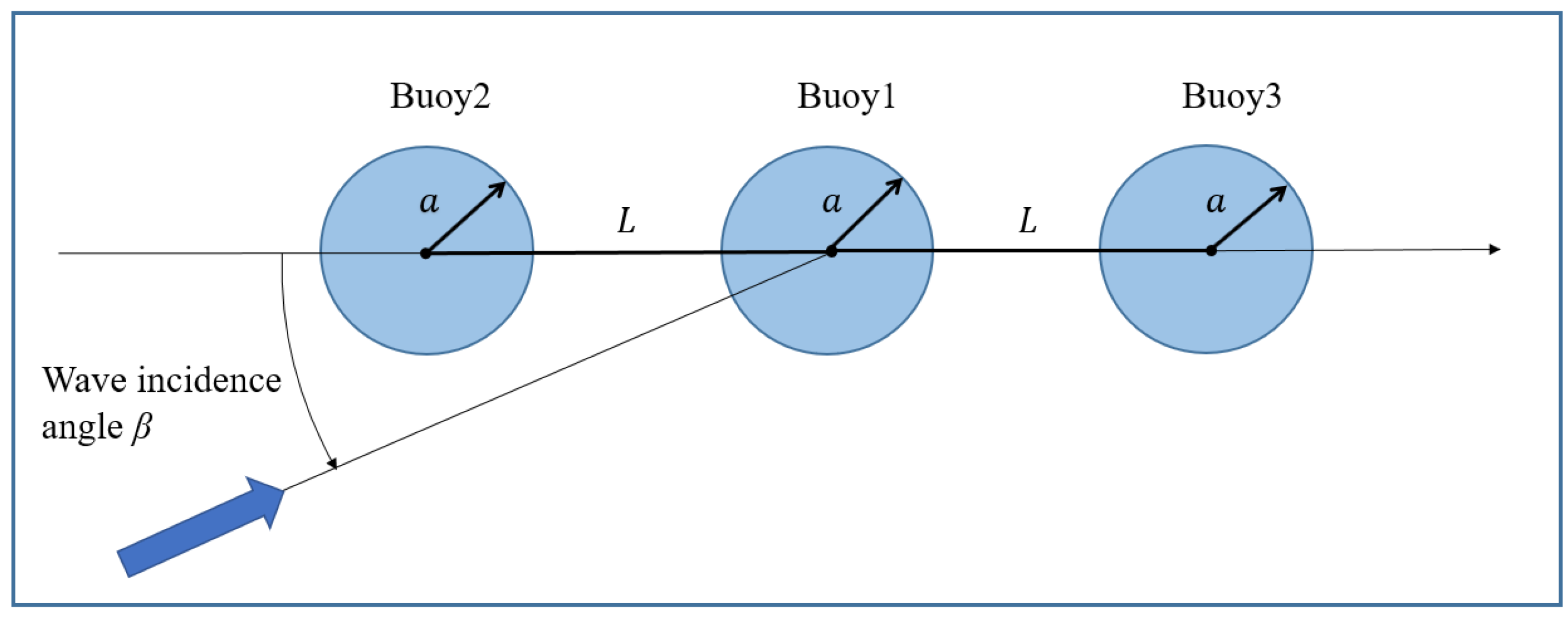
= 7 s, and the wave incidence angle β is selected as 0, 45, and 90 degrees to simulate the change in the wave incidence direction. According to the matching table of sea states and their optimal Cg, the optimal 
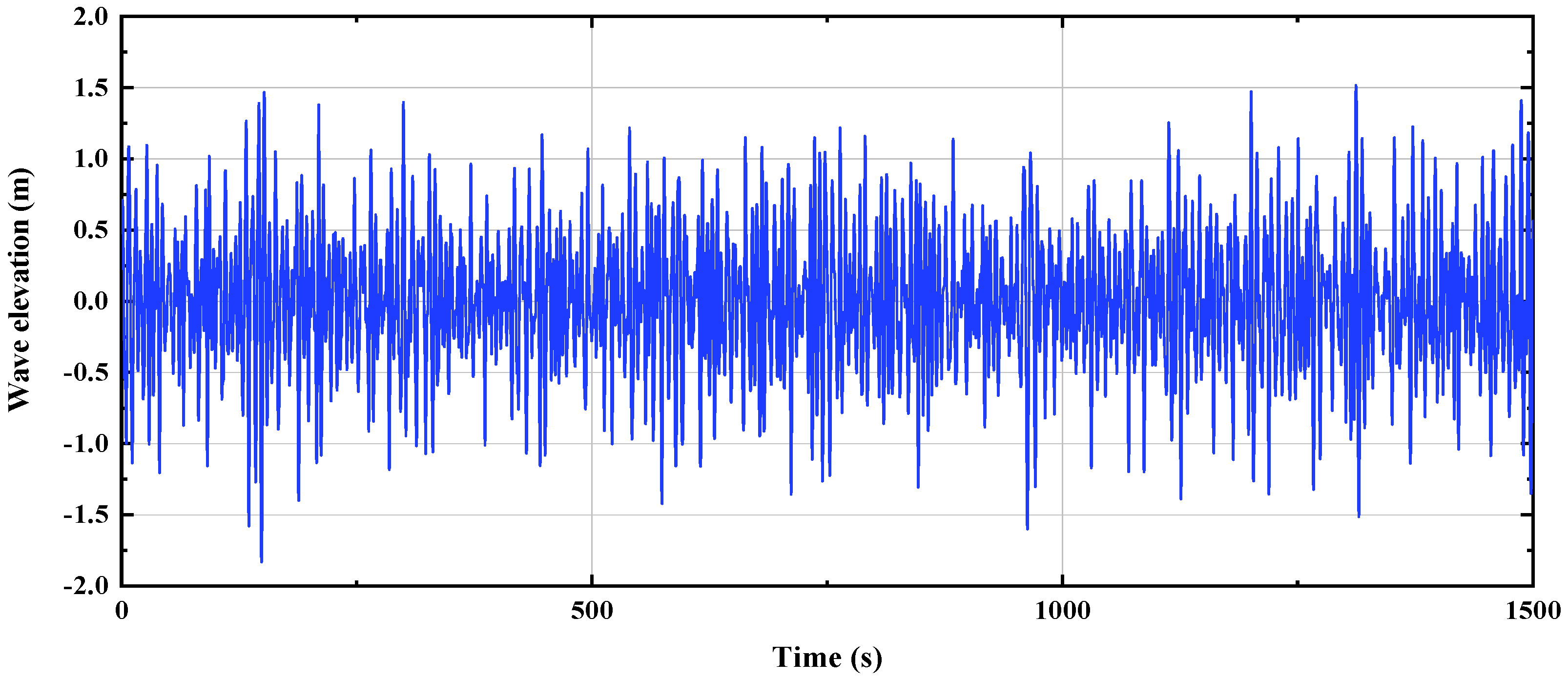
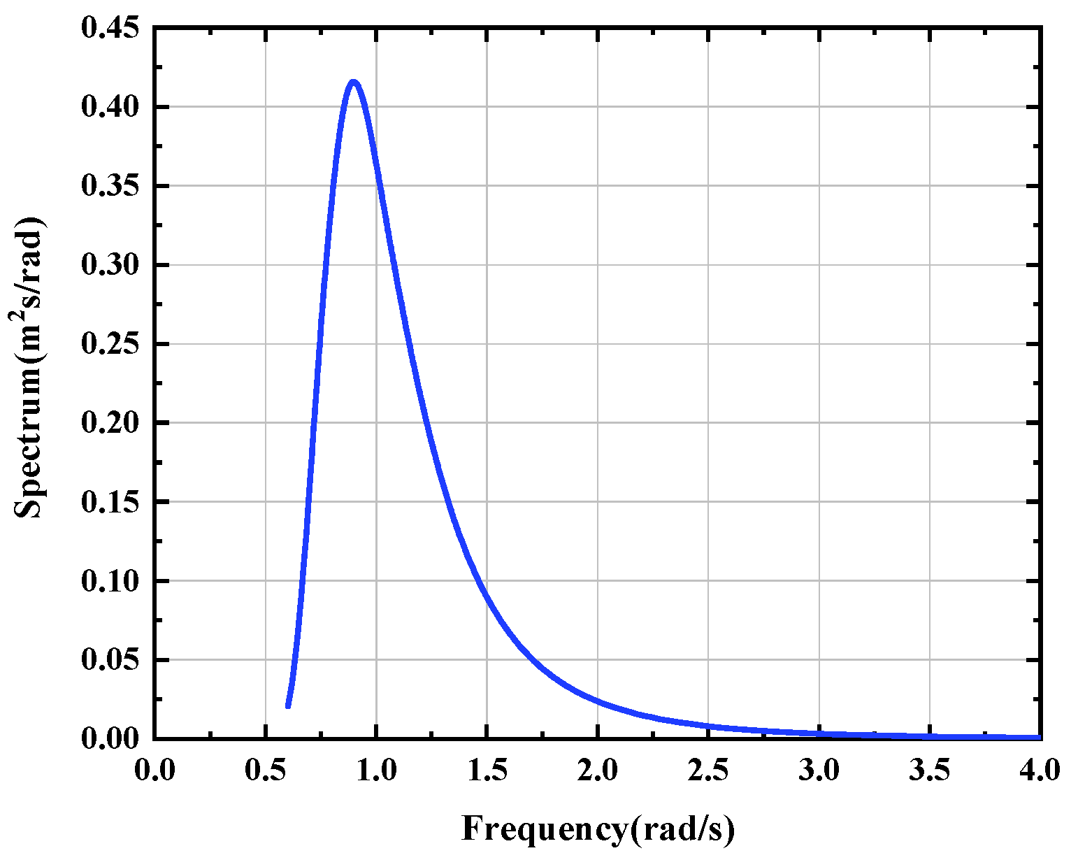
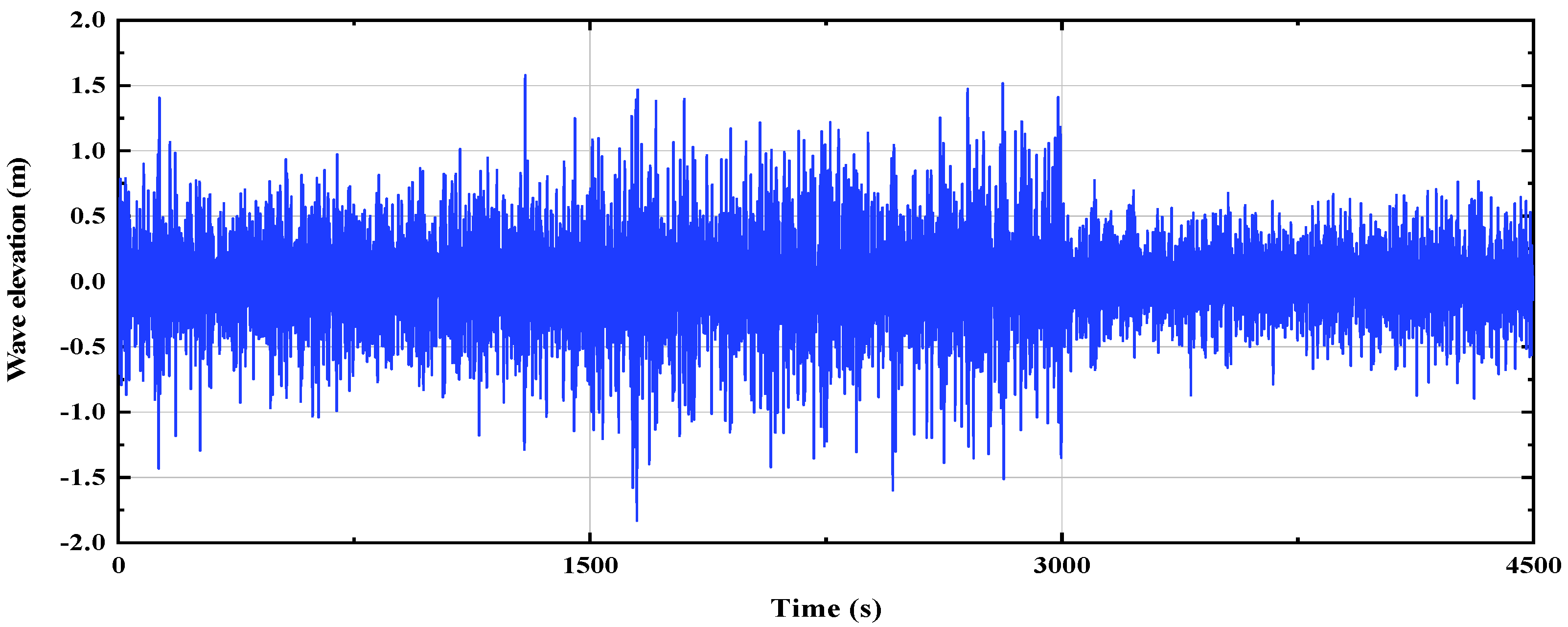
Cg for wave incidence angles of 0, 45, and 90 degrees are 45.4 N·m/(r/s), 48.5 N·m/(r/s), and 54.4 N·m/(r/s) respectively. For a given wave spectrum (JONSWAP spectrum), the time history of the irregular wave is generated by the linear superposition of harmonic wave components, and the wave elevation and the wave spectrum are shown in Figure 13 and Figure 14, respectively.
Table 6 shows the time average capture power without control ( P c u ) , the time average capture power with control ( P c ) , and the average capture power increase rate (γ) of the WEC array at different wave incidence angles. As can be seen in Table 6, when wave incidence angles are 0°, 45° and 90°, the average capture power of the array buoys is increased by 10.44%, 9.78%, and 8.34%, respectively, using the proposed control system, indicating that the proposed control system improves the energy capture characteristics of the array buoys even when the wave incidence direction is changed. And the average capture power of the array buoys increases with the increase in the wave incidence angle because the shielding effect between the array buoys is smaller with an increase in the wave incidence angle in the range of 0°~90°.
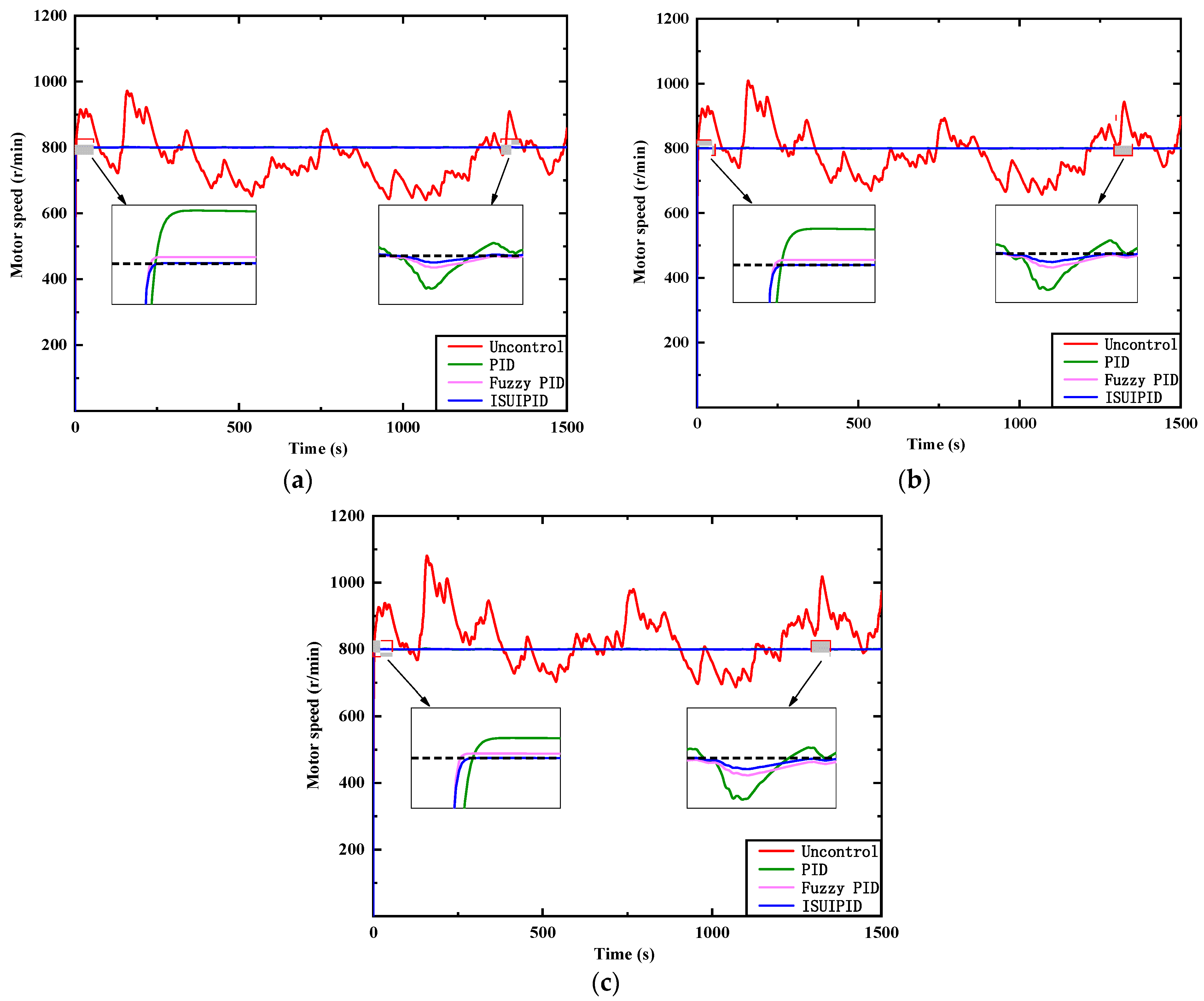
The output speeds of the hydraulic motor with the PID, the fuzzy PID, and the proposed ISUIPID controller at different wave incidence angles are shown in Figure 15, where the black dotted line is the ideal speed curve. The simulation results show that with the proposed control system, the output speed of the hydraulic motor tracks the rated speed well despite the change in the wave incidence direction. Compared with the PID and fuzzy PID controllers, the ISUPID controller has no overshoot and less tracking error. Table 7 shows the comparative analysis of the performance of various controllers at different wave incidence angles. The ISUIPID controller has the same rising time compared to the PID and fuzzy PID controllers. Since the initial speed of the motor is 0 and the initial tracking error is large, the hydraulic motor runs at its maximum displacement to quickly reduce the tracking error regardless of the controller. The ISUIPID controller has the best maximum absolute error and the best mean absolute error at each wave incidence angle compared to the PID and fuzzy PID controllers. When the incidence angle is 0°, 45° and 90°, the maximum absolute errors are reduced by 41.7%, 49.6%, and 50.8%, respectively, compared with the PID controller, and by 8.3%, 9.1%, and 14.5%, respectively, compared with the fuzzy PID controller. In addition, when the incidence angle is 0°, 45°, and 90°, the mean absolute errors are reduced by 79.6%, 79.0%, and 80.0%, respectively, compared with the PID controller, and by 40.0%, 38.1%, and 39.1%, respectively, compared with the fuzzy PID controller.
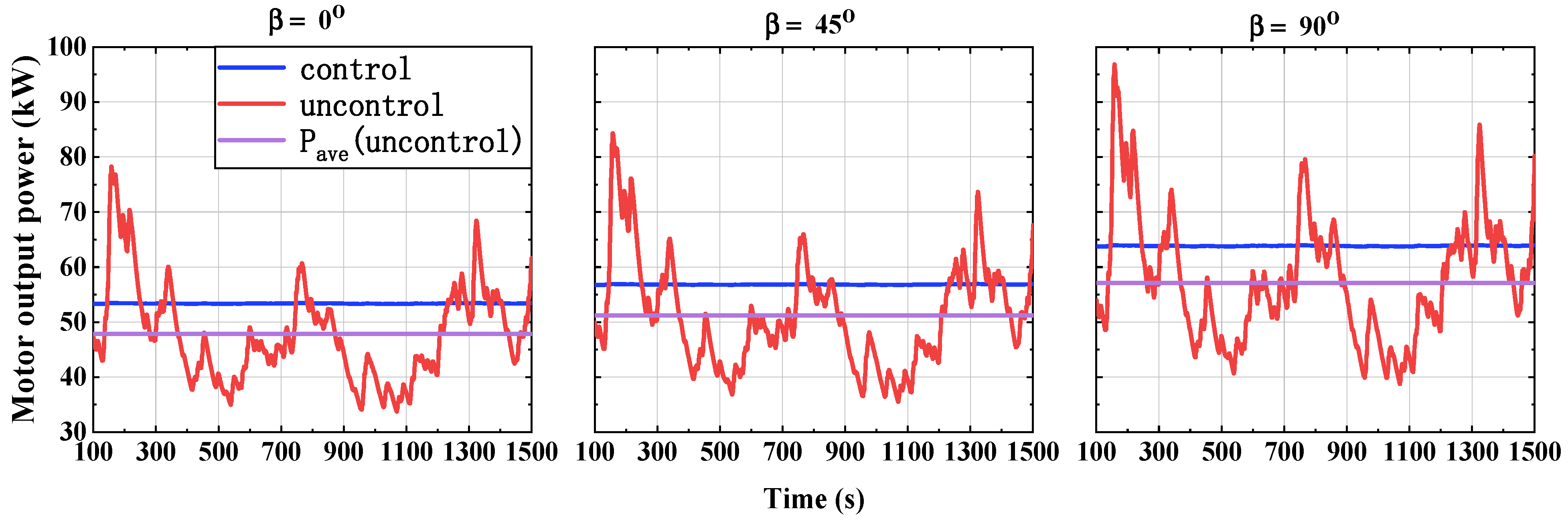
Figure 16 illustrates the output power of the hydraulic motor and Table 8 illustrates the time average output power without control ( P a v e ) , the output power with control ( P m ) , and the increased rate of output power (ζ) at different wave incidence angles. Under the proposed control system, the output power of the hydraulic motor is stable at each wave incidence angle, and the output power increases by 11.57%, 10.98%, and 11.75% when the wave incidence angles are 0°, 45°, and 90°, respectively, which demonstrates that the proposed control system can significantly increase and stabilize the output power of the WEC arrays even under sea conditions with large variations in wave direction.
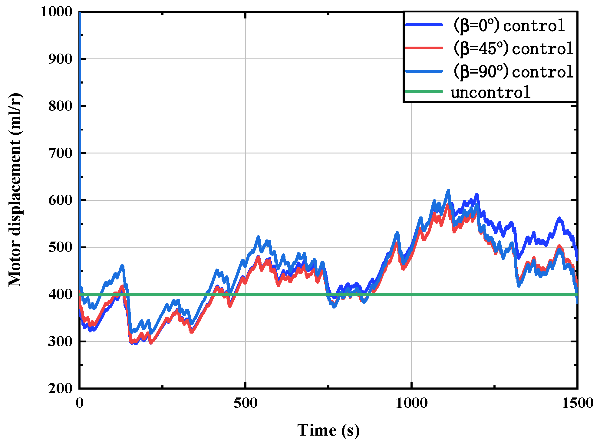
Figure 17 presents the displacement of the hydraulic motor with and without control at different wave incidence angles. As can be seen in Figure 17, the displacement of the hydraulic motor changes constantly to meet the ideal speed under the irregular incident wave. Since the initial speed of the hydraulic motor is 0 r/min, the motor displacement reaches the upper limit in the initial stage in order to rapidly reduce the large speed error in the initial stage. After the speed is stable, the hydraulic motor displacement fluctuates between 280 mL/r and 630 mL/r, which is in accordance with the actual operating requirements of the hydraulic motor.
2.
Significant wave height and energy period change.
In this section, the incident wave is an irregular wave composed of the following three wave states: (a) H s = 1.5 m and T e = 6 s; (b) H s = 2 m and T e = 7 s; (c) H s = 1 m and T e = 5 s. The operating time of each wave state is 1500 s, and the wave incidence angle is selected as 90°. Based on the matching table of sea states and their optimal Cg, the optimal 
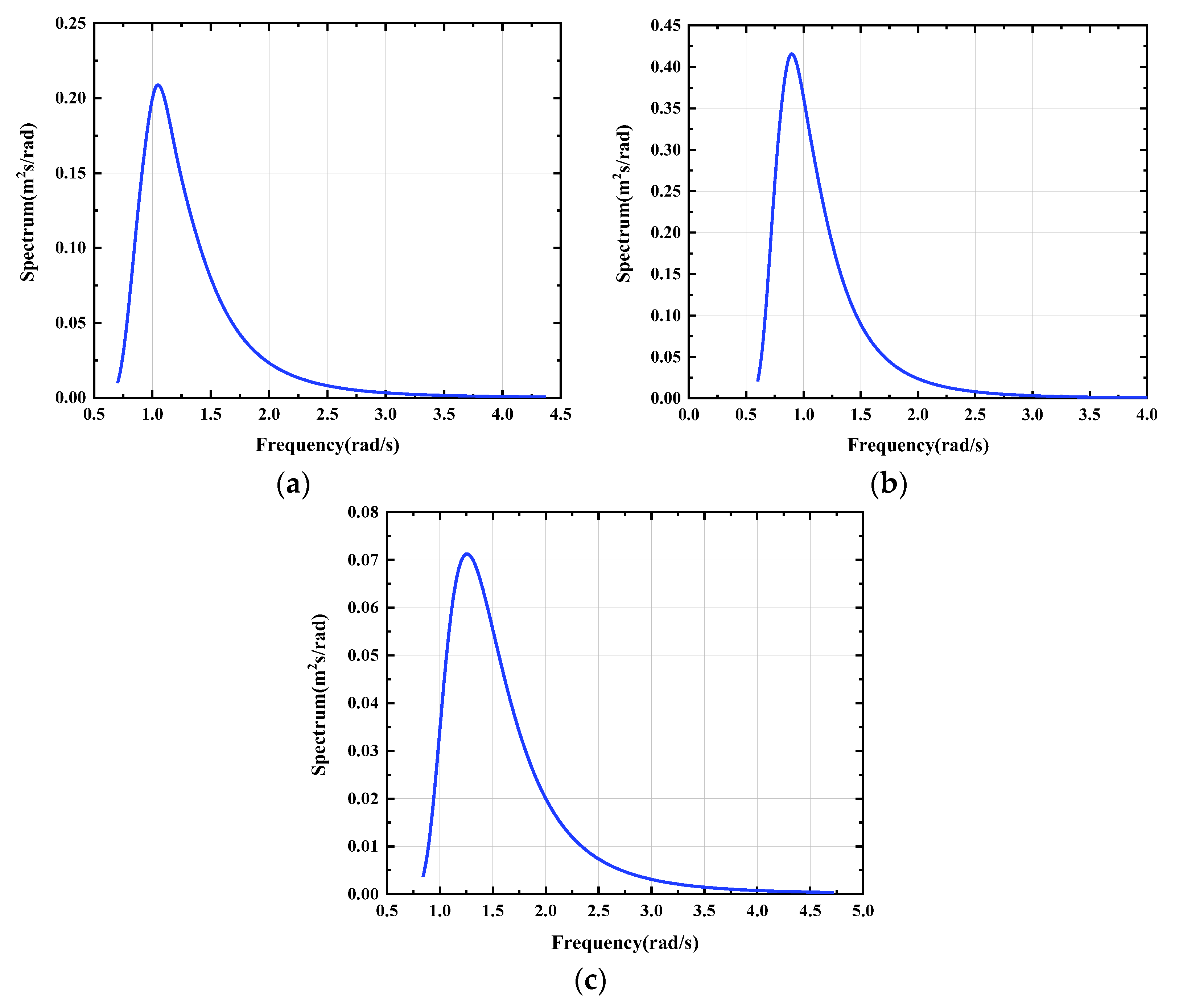
Cg for the above three wave states are 35.2 N·m/(r/s), 54.4 N·m/(r/s), and 19.8 N·m/(r/s), respectively. Then, the wave elevation and the wave spectra of the above wave state are shown in Figure 18 and Figure 19, respectively.
Table 9 displays the time average capture power without control ( P c u ), the time average capture power with control ( P c ), and the average capture power increase rate (γ) at different significant wave heights and energy periods. As shown, the average capture power of the array buoys is increased by 27.37%, 8.34%, and 41.83% using the proposed control system for the three wave states mentioned above, respectively, which indicates that the proposed control system is able to significantly improve the capture power of the arrayed buoys under various wave states, and the smaller the wave states are, the more obvious the enhancement effect is.
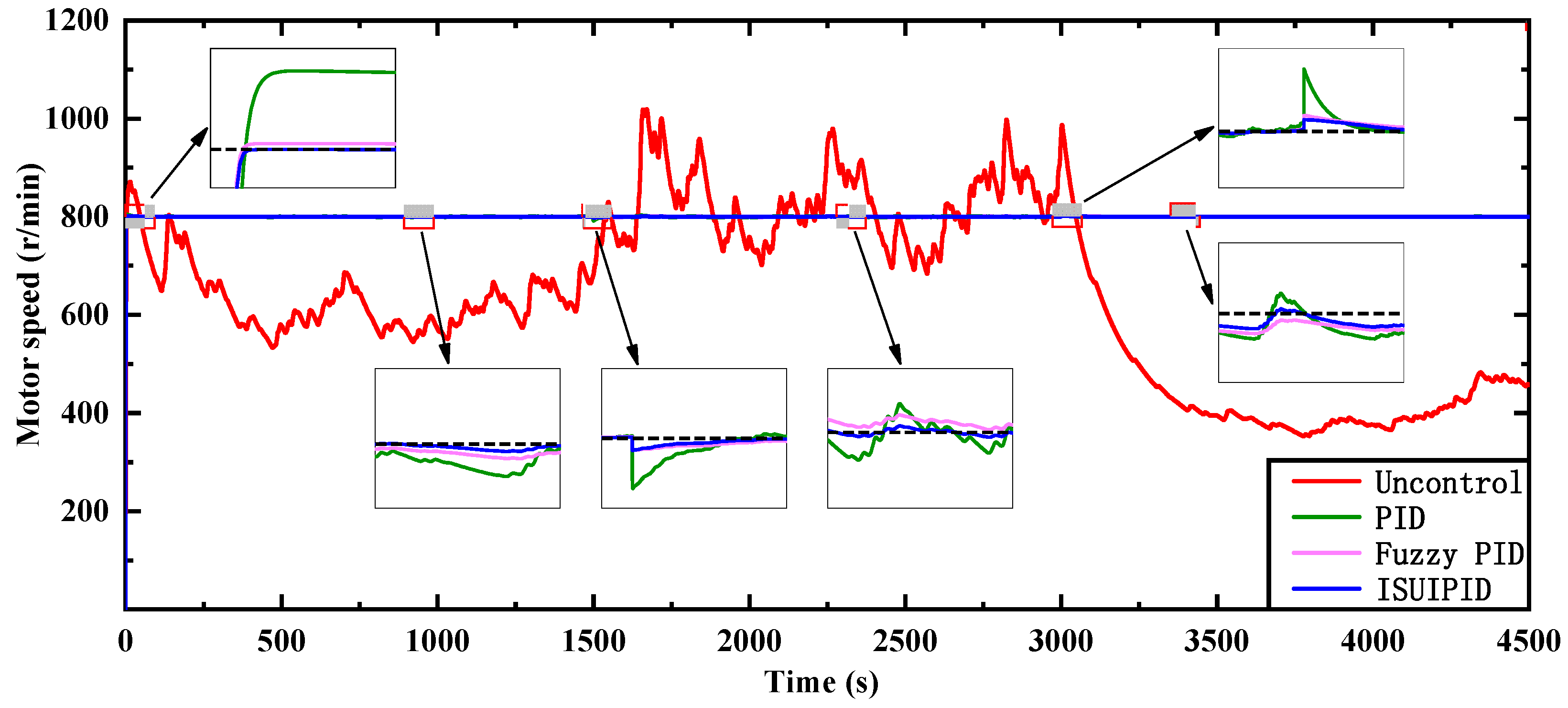
As shown in Figure 20, the output speed of the hydraulic motor has a good tracking effect under the action of the control system, which indicates that the proposed control system has excellent performance and strong robustness when the wave state changes. And compared with the PID and fuzzy PID controllers, the ISUPID controller has less overshoot during wave state change and less tracking error during the whole operation. The comparative analysis of the performance of various controllers at different wave states is shown in Table 10. The ISUIPID controller has the best maximum absolute error and the best mean absolute error throughout the operation as compared to the PID and fuzzy PID controllers. The maximum absolute error and the mean absolute error are reduced by 62.1%, and 75.0%, respectively, compared with the PID controller. And compared to the fuzzy PID controller, the maximum absolute error and the mean absolute error are reduced by 36.3% and 36.4%, respectively.
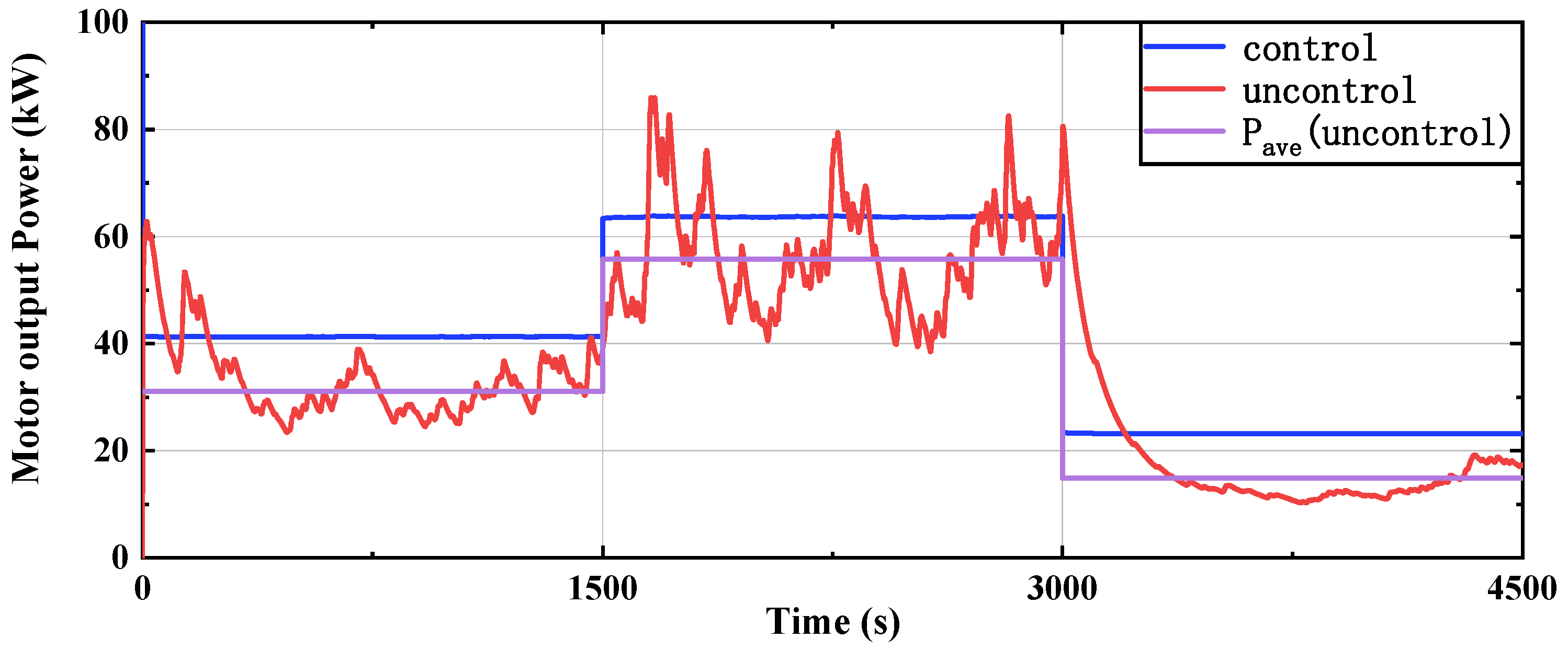
The output power of the hydraulic motor with and without control at different wave states is illustrated in Figure 21, and Table 11 shows the time average output power without control ( P a v e ), the output power with control ( P m ), and the increased rate of output power (ζ) at different wave incidence angles. It can be seen that the output power of the hydraulic motor is increased by 32.62%, 11.75%, and 55.91%, respectively, in these three wave states, and the power can be output stably in each wave state. This indicates that the proposed control system has a significant effect on improving the energy capture power of the array buoys as well as enhancing and stabilizing the output power of the array of PA-WECs, and the smaller the waves, the more obvious the improvement effect.
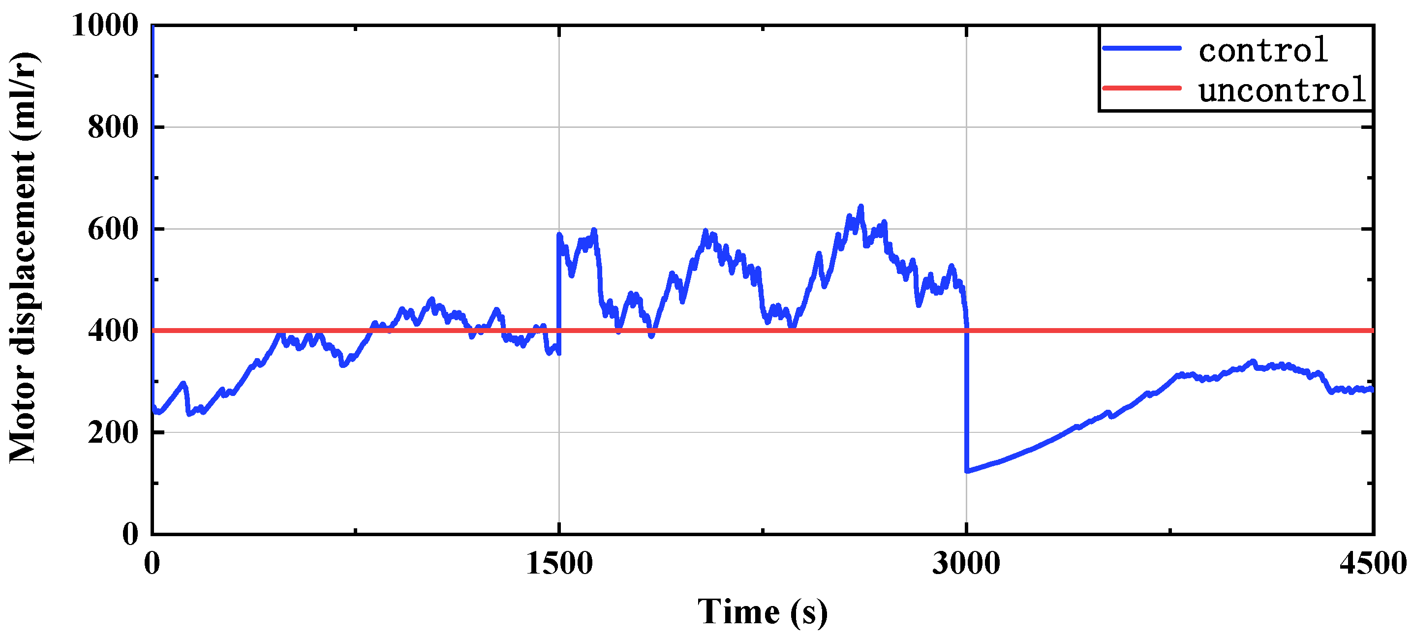
The displacement of the hydraulic motor with and without control at different wave states is shown in Figure 22. In order to track the rated speed of the hydraulic motor under the irregular incident wave, the displacement of the hydraulic motor varies continuously between 90 mL/r and 790 mL/r. The displacement of the hydraulic motor changes abruptly when the wave state changes and fluctuates within a relatively small range after the wave state stabilizes. This is because the change in wave state means that there is an abrupt change in the input to the WEC array, and the control system needs to quickly adjust the displacement of the hydraulic motor in order to keep the hydraulic motor running at the desired speed.

6. Conclusions

In this paper, a hydraulic PTO system for the array of PA-WECs has been designed and simulated. The mathematical model of the proposed system including the hydrodynamics of the array buoys and the hydraulic PTO system is presented. A new control system, including the ISUPID controller and the adaptive matching controller using IGTO, is designed. The performance of the proposed hydraulic PTO system and the control system is investigated under irregular wave states with different significant wave heights, energy periods, and wave incidence angles. Based on the investigation and analysis, the following conclusions can be extracted:
  • The designed IGTO optimization algorithm has a great improvement in convergence speed and accuracy, which provides a faster and more accurate optimization method for the optimization of the Cg for WECs and other related optimization problems.
  • The proposed ISUIPID controller has superior performance in tracking the desired speed of the hydraulic motor under irregular waves with changing wave conditions compared with the PID and fuzzy PID controllers. Under three different wave incidence angles and the sea state composed of three irregular waves with different significant wave heights and energy periods, the mean absolute error of the ISUIPID controller is 79.6%, 79.0%, 80.0%, and 75.0% lower, respectively, compared with the PID controller, and 40.0%, 38.1%, 39.1%, and 36.4% lower, respectively, compared with the fuzzy PID controller.
  • The proposed control system has shown significant benefits in improving the energy capture power of the array buoys as well as enhancing and stabilizing the output power of the array of PA-WECs. The capture power is increased by 10.44%, 9.78%, 8.34%, 27.37%, 8.34%, and 41.83%, respectively, and the output power is increased by 11.57%, 10.98%, 11.75%, 32.62%, 11.75%, and 55.91%, respectively, under the three wave directions and three wave states considered in this paper.
The present study provides a simple and efficient hydraulic PTO system and a simple, intelligent, and engineering-applicable control system for arrays of WECs. In addition, the proposed control system can be applied to a single WEC with a hydraulic PTO system. As a result, the designed system will lead the WEC array or WEC to become an independent, stable, efficient, and sustainable power generation system.

Author Contributions

Conceptualization, D.W.; methodology, D.W.; software, D.W.; validation, D.W., Y.H., and Z.Z.; formal analysis, D.W.; investigation, Y.H.; resources, G.X.; data curation, Z.Z.; writing—original draft preparation, D.W.; writing—review and editing, G.X.; visualization, D.W.; supervision, Y.L.; project administration, Y.L.; funding acquisition, Y.L. All authors have read and agreed to the published version of the manuscript.

Funding

This work was funded by the National Natural Science Foundation of China, grant number 52171265, and the Natural Science Foundation of Shandong Province, grant number ZR2021ZD23.

Institutional Review Board Statement

Not applicable.

Informed Consent Statement

The study did not involve humans.

Data Availability Statement

Data are available on request due to restrictions e.g., privacy or ethical. The data presented in this study are available on request from the corresponding author. The data are not publicly available due to the presence of some confidential information.

Conflicts of Interest

The authors declare no conflict of interest.

References

  1. Cruz, J. Ocean Wave Energy: Current Status and Future Perspectives; Green Energy Technology Series; Springer: Berlin/Heidelberg, Germany, 2008. [Google Scholar]
  2. Lehmann, M.; Karimpour, F.; Goudey, C.A.; Jacobson, P.T.; Alam, M.R. Ocean wave energy in the united states: Current status and future perspectives. Renew. Sustain. Energy Rev. 2020, 74, 1300–1313. [Google Scholar] [CrossRef]
  3. Falco, A.F.d.O. Wave energy utilization: A review of the technologies. Renew. Sustain. Energy Rev. 2010, 14, 899–918. [Google Scholar] [CrossRef]
  4. Rusu, E.; Onea, F. A review of the technologies for wave energy extraction. Clean Energy 2018, 2, 10–19. [Google Scholar] [CrossRef]
  5. Gallutia, D.; Fard, M.T.; Soto, M.G.; He, J.B. Recent advances in wave energy conversion systems: From wave theory to devices and control strategies. Ocean Eng. 2022, 252, 111105. [Google Scholar] [CrossRef]
  6. Soares, C.G.; Bhattacharjee, J.; Tello, M.; Pietra, L. Review and Classification of Wave Energy Converters; Marine Engineering and Technology: London, UK, 2012; pp. 585–594. [Google Scholar]
  7. Haraguchi, R.; Asai, T. Enhanced power absorption of a point absorber wave energy converter using a tuned inertial mass. Energy 2020, 202, 117740. [Google Scholar] [CrossRef]
  8. Ruezga, A.; José, M.; Cañedo, C. Buoy Analysis in a Point-Absorber Wave Energy Converter. IEEE J. Ocean. Eng. 2020, 45, 472–479. [Google Scholar] [CrossRef]
  9. Korde, U.A.; Ringwood, J. Hydrodynamic Control of Wave Energy Devices; Cambridge University Press: Cambridge, UK, 2016. [Google Scholar]
  10. Zhang, Z.; Qin, J.; Wang, D.; Wang, W.; Liu, Y.; Xue, G. Research on wave excitation estimators for arrays of wave energy converters. Energy 2023, 264, 126133. [Google Scholar] [CrossRef]
  11. Ruehl, K.; Bull, D. Wave energy development roadmap: Design to commercialization. In Proceedings of the OCEANS 2012, Hampton Roads, VA, USA, 14–19 October 2012; pp. 1–10. [Google Scholar]
  12. Rui, P.; Gato, L.; Henriques, J.; Portillo, J.; Greaves, D.M. Compact floating wave energy converters arrays: Mooring loads and survivability through scale physical modelling. Appl. Energ. 2020, 280, 115982. [Google Scholar]
  13. Andres, A.D.D.; Guanche, R.; Meneses, L.; Vidal, C.; Losada, I.J. Factors that influence array layout on wave energy farms. Ocean Eng. 2014, 82, 32–41. [Google Scholar] [CrossRef]
  14. Lyu, J.; Abdelkhalik, O.; Gauchia, L. Optimization of dimensions and layout of an array of wave energy converters. Ocean Eng. 2019, 192, 106543. [Google Scholar] [CrossRef]
  15. Faedo, N.; Pea-Sanchez, Y.; Ringwood, J.V. Parametric representation of arrays of wave energy converters for motion simulation and unknown input estimation: A moment-based approach. Appl. Ocean Res. 2020, 98, 102055. [Google Scholar] [CrossRef]
  16. Zou, S.; Abdelkhalik, O. Collective control in arrays of wave energy converters. Renew. Energy 2020, 156, 361–369. [Google Scholar] [CrossRef]
  17. Murai, M.; Li, Q.; Funada, J. Study on power generation of single Point Absorber Wave Energy Converters (PA-WECs) and arrays of PA-WECs. Renew. Energy 2016, 86, 1121–1132. [Google Scholar] [CrossRef]
  18. Gaspar, J.F.; Calvário, M.; Kamarlouei, M.; Soares, C.G. Power take-off concept for wave energy converters based on oil-hydraulic transformer units. Renew. Energy 2021, 164, 1121–1246. [Google Scholar] [CrossRef]
  19. Do, H.T.; Dang, T.D.; Ahn, K.K. A multi-point-absorber wave-energy converter for the stabilization of output power. Ocean Eng. 2018, 161, 337–349. [Google Scholar] [CrossRef]
  20. Gaspar, J.F.; Kamarlouei, M.; Sinha, A. Speed control of oil-hydraulic power take-off system for oscillating body type wave energy converters. Renew. Energy 2016, 97, 769–783. [Google Scholar] [CrossRef]
  21. Fan, Y.; Mu, A.; Ma, T. Design and control of a point absorber wave energy converter with an open loop hydraulic transmission. Energy Convers. Manag. 2016, 121, 13–21. [Google Scholar] [CrossRef]
  22. Geng, D.; Zheng, Y.; Chen, Q.; Yue, X.; Yan, D. Novel hydraulic mechanism-based output power regulation for the wave energy converter. APL Ocean Res. 2021, 110, 102587. [Google Scholar] [CrossRef]
  23. Chen, Q.; Yan, D.; Zheng, Y.; Yue, X.; Geng, D. Operation characteristics and methods of the hydraulic power take-off system. Trans. Inst. Meas. Control 2021, 43, 137–150. [Google Scholar] [CrossRef]
  24. Zhong, Q. Hydrodynamic Modeling, Optimal Control, and Performance Evaluation of an Array of Ocean-Wave Energy Converters. Ph.D. Thesis, University of California, Los Angeles, CA, USA, 2018. [Google Scholar]
  25. Wehausen, J.D. The motion of floating bodies. Annu. Rev. Fluid Mech. 1971, 3, 237–268. [Google Scholar] [CrossRef]
  26. Babarit, A.; Muliawan, M.; Hals, J.; Kurniawan, A.; Moan, T. Numerical benchmarking study of a selection of wave energy converters. Renew. Energy 2012, 41, 44–63. [Google Scholar] [CrossRef]
  27. El-Khatib, M.F.; Sabry, M.; EI-Sebah, M.I.; Maged, S.A. Hardware-in-the-loop testing of simple and intelligent MPPT control algorithm for an electric vehicle charging power by photovoltaic system. ISA Trans. 2023, 137, 656–669. [Google Scholar] [CrossRef] [PubMed]
  28. Sebah, M. Simplified intelligent universal PID controller. Int. J. Eng. Res. 2016, 5, 11–15. [Google Scholar]
  29. Falnes, J. Ocean Waves and Oscillating Systems; Cambridge University Press: Cambridge, UK, 2005. [Google Scholar]
  30. Abdollahzadeh, B.; Soleimanian Gharehchopogh, F.; Mirjalili, S. Artificial gorilla troops optimizer: A new nature-inspired metaheuristic algorithm for global optimization problems. Int. J. Intel. Syst. 2021, 36, 5887–5958. [Google Scholar] [CrossRef]
  31. Ginidi, A.; Ghoneim, S.M.; Elsayed, A.; El-Sehiemy, R.; Shaheen, A.; EI-Fergany, A. Gorilla troops optimizer for electrically based single and double-diode models of solar photovoltaic systems. Sustainability 2021, 13, 9459. [Google Scholar] [CrossRef]
  32. Haupt, R.; Haupt, S. Practical Genetic Algorithm; John Wiley and Sons: Hoboken, NJ, USA, 2004; pp. 51–65. [Google Scholar]
Figure 1. Schematic of an example of the proposed array of PA-WECs.
Sustainability 15 16092 g001
Figure 2. Basic architecture of the control system for arrays of WECs.
Sustainability 15 16092 g002
Figure 3. Control architecture of the ISUIPID controller.
Sustainability 15 16092 g003
Figure 4. Control architecture of the intelligent PID controller.
Sustainability 15 16092 g004
Figure 5. Control architecture of the hydraulic motor speed using the ISUIPID controller.
Sustainability 15 16092 g005
Figure 6. Control architecture of the hydraulic motor speed using the fuzzy PID controller.
Sustainability 15 16092 g006
Figure 7. Control architecture of the adaptive matching controller.
Sustainability 15 16092 g007
Figure 8. Simulation model of the array of WECs.
Sustainability 15 16092 g008
Figure 9. Flowchart of the proposed IGTO algorithm.
Sustainability 15 16092 g009
Figure 10. Layout diagram of the array of WECs.
Sustainability 15 16092 g010
Figure 11. Simulink block diagram of the proposed system.
Sustainability 15 16092 g011
Figure 12. The convergence curves of the Cg optimization problem under five sea states. (a) H s = 1 m, T e = 5 s, β = 90°; (b) H s = 1.5 m, T e = 6 s, β = 90°; (c) H s = 2 m, T e = 7 s, β = 90°; (d) H s = 2 m, T e = 7 s, β = 45°; (e) H s = 2 m, T e = 7 s, β = 0°.
Sustainability 15 16092 g012aSustainability 15 16092 g012b
Figure 13. Wave elevation for the irregular wave of H s = 2 m and T e = 7 s.
Sustainability 15 16092 g013
Figure 14. Wave spectrum for the irregular wave of H s = 2 m and T e = 7 s.
Sustainability 15 16092 g014
Figure 15. Output speed of the hydraulic motor at different wave incidence angles. (a) Output speed of the hydraulic motor at 0° wave incidence angle; (b) output speed of the hydraulic motor at 45° wave incidence angle; (c) output speed of the hydraulic motor at 90° wave incidence angle.
Sustainability 15 16092 g015
Figure 16. Output power of the hydraulic motor at different wave incidence angles.
Sustainability 15 16092 g016
Figure 17. Displacement of the hydraulic motor at different wave incidence angles.
Sustainability 15 16092 g017
Figure 18. Wave elevation of the above wave state.
Sustainability 15 16092 g018
Figure 19. Wave spectra of the above wave state. (a) H s = 1.5 m and T e = 6 s; (b) H s = 2 m and T e = 7 s; (c) H s = 1 m and T e = 5 s.
Sustainability 15 16092 g019
Figure 20. Output speed of the hydraulic motor at different wave states.
Sustainability 15 16092 g020
Figure 21. Output power of the hydraulic motor at different wave states.
Sustainability 15 16092 g021
Figure 22. Displacement of the hydraulic motor of the hydraulic motor at different wave states.
Sustainability 15 16092 g022
Table 1. The fuzzy rules of K p , K i , and K d .
e c F Proportional   Coefficient   K p Integral   Coefficient   K i Differential   Coefficient   K d
e F = ZEPSPMPBZEPSPMPBZEPSPMPB
ZEZEPSPMPBPBPBPMZEPSPSPSZE
PSZEPSPMPBPBPBPMZEZEZEZEZE
PMZEPSPMPBPBPMPSZEPSPSPSPB
PBZEZEPSPMPMPMPSZEPMPSPSPB
Table 2. The parameters of the hydraulic PTO system.
ParameterSymbolValueUnit
Inner diameter of the hydraulic cylinder D 0 180mm
Rod diameter of the piston rod d 0 140mm
Initial gas pressure of the accumulator P 0 5.3MPa
Initial gas volume of the accumulator V 0 3L
Rated speed of the motor (ideal speed) n r 800r/min
Mechanical efficiency of the motor η m 0.9/
Volumetric efficiency of the motor η V 0.9/
Adjustment range of the motor displacement V m r 0~1000mL/r
Rotational inertia of the motor J m 3 k g · m 2
Rotational inertia of the generator rotor J g 7 k g · m 2
Table 3. The parameters of the controllers.
The ISUIPID ControllerThe Fuzzy PID ControllerThe PID Controller
K 1 = 1290 K e = 0.00125 K u 1 = 0.9 K p = 0.00003
K 2 = 4.9 K e c = 0.00125 K u 2 = 0.00165 K i = 0.0000018
K u = 1 K u 3 = 0.00019 K d = 0.00000015
Table 4. Parameters settings for each algorithm.
AlgorithmParameter
IGTOp = 0.03, β = 3, W = 0.8, N = 40, MaxIt = 100
GTOp = 0.03, β = 3, W = 0.8, N = 40, MaxIt = 100
GAPc = 0.9, Pm = 0.01, N = 40, MaxIt = 100
PSOc = 2.0, w = 0.9, N = 40, MaxIt = 100
Table 5. The matching table of the five sea states and their optimal Cg.
SEA STATESOptimal CgMaximized Average Output Power
H s = 1 m, T e = 5 s, β = 90°19.8 N·m/(r/s)23.23 kW
H s = 1.5 m, T e = 6 s, β = 90°35.2 N·m/(r/s)41.35 kW
H s = 2 m, T e = 7 s, β = 90°54.4 N·m/(r/s)63.84 kW
H s = 2 m, T e = 7 s, β = 45°48.5 N·m/(r/s)56.91 kW
H s = 2 m, T e = 7 s, β = 0°45.4 N·m/(r/s)53.33 kW
Table 6. P c u and P c at different wave incidence angles.
Wave Incidence Angles45°90°
Time average capture power without control P c u (kW)48.8652.4359.58
Time average capture power with control P c (kW)53.9657.5664.55
Average capture power increase rate γ10.44%9.78%8.34%
Table 7. Comparison of the performance of several controllers at different wave incidence angles.
Wave
Incidence Angles
Rising TimeMaximum Absolute ErrorMean Absolute Error
PIDFuzzy PIDISUIPIDPIDFuzzy PIDISUIPIDPIDFuzzy PIDISUIPID
0.490.490.491.030.600.550.590.200.12
45°0.500.500.501.190.660.600.620.210.13
90°0.510.510.511.320.760.650.700.230.14
Table 8. P a v e and P m at different wave incidence angles.
Wave Incidence Angles45°90°
Time average output power without control P a v e (kW)47.8051.2857.13
Output power with control P m (kW)53.3356.9163.84
Increase rate of output power ζ11.57%10.98%11.75%
Table 9. P c and P c u at different significant wave heights and energy periods.
Wave Condition H s = 1.5   m , T e = 6   s H s = 2   m , T e = 7   s H s = 1   m , T e = 5   s
P c u (kW)33.159.5817.5
P c (kW)42.1664.5524.82
γ27.37%8.34%41.83%
Table 10. Comparison of the performance of several controllers at different wave states.
Rising TimeMaximum Absolute ErrorMean Absolute Error
PIDFuzzy PIDISUIPIDPIDFuzzy PIDISUIPIDPIDFuzzy PIDISUIPID
0.460.460.461.530.910.580.560.220.14
Table 11. P a v e and P m at different wave states.
Wave Condition H s = 1.5   m , T e = 6   s H s = 2   m , T e = 7   s H s = 1   m , T e = 5   s
P a v e (kW)31.1857.1314.90
P m (kW)41.3563.8423.23
ζ32.62%11.75%55.91%
Disclaimer/Publisher’s Note: The statements, opinions and data contained in all publications are solely those of the individual author(s) and contributor(s) and not of MDPI and/or the editor(s). MDPI and/or the editor(s) disclaim responsibility for any injury to people or property resulting from any ideas, methods, instructions or products referred to in the content.

