Application of Wavelet Transform for Bias Correction and Predictor Screening of Climate Data

Abstract

Climate model (CM) statistical downscaling requires quality and quantity modifications of the CM’s outputs to increase further modeling accuracy. In this respect, multi-resolution wavelet transform (WT) was employed to determine the hidden resolutions of climate signals and eliminate bias in a CM. The results revealed that the newly developed discrete wavelet transform (DWT)-based bias correction method can outperform the quantile mapping (QM) method. In this study, wavelet coherence analysis was utilized to assess the high common powers and the multi-scale correlation between the predictors and predictand as a function of time and frequency. Thereafter, to rate the most contributing predictors based on potential periodicity, the average variance was calculated, which is named the Scaled Average (SA) measure. Consequently, WT along with Artificial Neural Network (ANN) were applied for bias correction and identifying the dominant predictors for statistical downscaling. The CAN-ESM5 data of Canadian climate models and INM-CM5 data of Russian climate models over two climatic areas of Iran with semi-arid (Tabriz) and humid (Rasht) weather were applied. The projection of future precipitation revealed that Tabriz will experience a 3.4–6.1% decrease in precipitation, while Rasht’s precipitation will decrease by 1.5–2.5%. These findings underscore the importance of refining CM data and employing advanced techniques to assess the potential impacts of climate change on regional precipitation patterns.

1. Introduction

The importance of sustainability becomes even more crucial in the face of future rainfall changes induced by climate change, as sustainable practices can help mitigate the negative impacts and ensure a more resilient and balanced water cycle for generations to come. To this end, the application of climate models (CMs), which provide hydro-meteorological information, is very important. However, the coarse spatial resolution of CM outputs is one of its main shortcomings, since several geographic features can be missed or not represented. Various downscaling methods have been applied to CM data to acquire local or regional scales [1], categorized as dynamic and statistical downscaling. Dynamic downscaling applies CM outputs to develop regional climate models (RCMs) with higher resolutions. However, statistical downscaling involves deriving relationships between large-scale climate data (predictors) and local-scale observed variables (predictands). Since statistical methods do not need physical information about the study area, this method is applicable in various geographic locations even without information on regional conditions [2].

In the literature, various statistical downscaling methods have been used, including multi-linear regression (MLR) models [3], weather generators (WGs), and nonlinear regression, namely, artificial intelligence (AI). The Support Vector Machine (SVM), Adaptive Neuro-Fuzzy Inference System (ANFIS) [4], Convolutional Neural Network (CNN) [5], and Artificial Neural Network (ANN) [6] are among the AI algorithms that have been used to downscale climate variables statistically.

As a robust and resilient tool, ANN has been applied to analyzing nonlinear relationships between hydro-climatic variables and downscaling CM data over the last few years [7,8,9]. Throughout 2011–2050, Su et al. applied ANN to predict variation in streamflow and precipitation [10]. Alotaibi et al. projected the future rainfall and temperatures of an arid area via ANN [11]. Prathom and Champrasert predicted the precipitation and temperature of their case study in Thailand using ANN along with a interpolation technique [12].

It should be noted that besides the positive application of ANN in statistical downscaling, some contradictory reports on using machine learning techniques (e.g., ANN) were also seen among different research. There is a reason for these contrary results, which may be related to the quality and quantity of datasets used in ANN modeling. A bias correction method is used to resolve the first issue and a data dimension reduction technique is applied to address the second drawback causing low performance.

Although CMs are used to project future climate variables, their output is accompanied by uncertainties due to systematic biases and errors [13,14]. Generally, these biases are due to difficulty in parametrizing convection processes, the inaccurate modeling of natural features such as mountains, or an inability to incorporate probable large-scale and influential climate variations that may cause disparate phases [15]. This problem has been addressed in the literature through a variety of approaches. There were various bias correction methods reviewed and compared by Teutschbein and Seibert, including linear scaling, local intensity scaling, power transformation, variance scaling, distribution transfer, and delta-change methods [13]. One of the most renowned and widely applied bias correction techniques is delta change, which modifies the mean values of datasets based on observation and historical periods [16]. Another widely used, more robust method is quantile mapping (QM). With this technique, the Cumulative Distribution Functions (CDF) of two datasets are fitted together to calibrate their probability distributions as well as their mean values [17]. Rajczak et al. compared QM with weather generators (WGs) and raw CM in precipitation simulations [18]. Hassanzadeh et al. conducted a comparison of three QM approaches for downscaling future rainfall extremes [19]. Gumus et al. implemented QM, detrended quantile mapping (DQM), and quantile delta mapping (QDM) as their bias correction method [20].

Data redundancy and reduced efficacy of ANN-based models can be associated with large input datasets [21]. Thus, large datasets of the CM should be pre-processed to identify dominant large-scale variables. Due to the synthesis of astronomical forcing and internal feedback, many geophysical datasets are characterized as non-stationary, with climate modes controlling the variability of the datasets [22]. The outputs of CMs are time series with non-stationary characteristics. Various methods have been used to detect and eliminate this non-stationarity that is presented in the literature [4,23]. Ahmadi and Han developed a hybrid model using gamma distribution and Coefficient Correlation (CC) for predicting precipitation [24]. The correlation analysis was used by Sachindra et al. to identify the dominant variables of the GCM [25]. As part of the downscaling process, the mutual information (MI) was compared with linear CC to pick dominant predictors [26]. Devak and Dhanya examined the effectiveness of Principal Component Analysis (PCA) as a dimension reduction before the statistical downscaling of CMs [27].

In various studies, wavelet analysis has been successfully applied to investigate non-stationary signals in hydrological processes [28]. Continuous wavelet transform (CWT) was used by Rana and Moradkhani to analyze downscaled precipitation and temperature data [29]. For downscaling MIROC5, Nguyen et al. used a frequency-based approach and concluded that it could be used to assess climate change impacts [30]. Recently, discrete wavelet transform (DWT) and wavelet entropy (WE) were used in research to determine dominant predictors [31].

To screen and draw features from large datasets, correlation-based analysis is a conventional technique. However, this method is not capable of detecting nonlinear relationships between time series. Since hydro-climatic variables have non-stationary and non-linear properties, traditional correlation methods cannot provide satisfactory results. In this respect, wavelet coherence analysis has been used in various studies to investigate the connection between two non-stationary signals. Maraun and Kurths used WTC analysis as a reliable method to expose local-scale correlations [32]. According to Jevrejeva et al., the WTC method was effective in identifying atmospheric circulation patterns in a study on the impacts of the Arctic Oscillation (AO) and North Atlantic Oscillation (NAO) on Baltic Sea ice [33]. Grinsted et al. examined the relationship between the climatic variables of the seas via WTC [34]. Also, wavelet correlation was investigated by Ng and Chan to evaluate the impacts of the El Nino–Southern Oscillation on tropical cyclone activity [35]. Tamaddun et al. assessed relevant oceanic–atmospheric parameters in snow water using WTC [36]. In earlier work, Nourani et al. employed WTC to evaluate the influence of hydroclimatological variables on Urmia Lake fluctuations [31]. It appears that no studies have been conducted that use WTC as a feature extraction method to reduce data dimensionality as part of the investigation of hydroclimatological processes.

Despite the growing literature on wavelet analysis, it appears that it has not been used for CM bias correction and predictor screening. Therefore, DWT was employed to eliminate biases in climate model outputs, and its results were compared with those of QM for two study areas with humid and semi-arid climate conditions. The WTC method was applied to reduce data dimensionality and to select the dominant predictors affecting precipitation. A comparison between WTC and the traditional CC methodology was also conducted. The three methods were then analyzed using an ANN model to compare their performance in downscaling precipitation, and the study areas were projected based on a downscaling model using two CMs (INM-CM5 and CAN-ESM5).

2. Materials and Methods

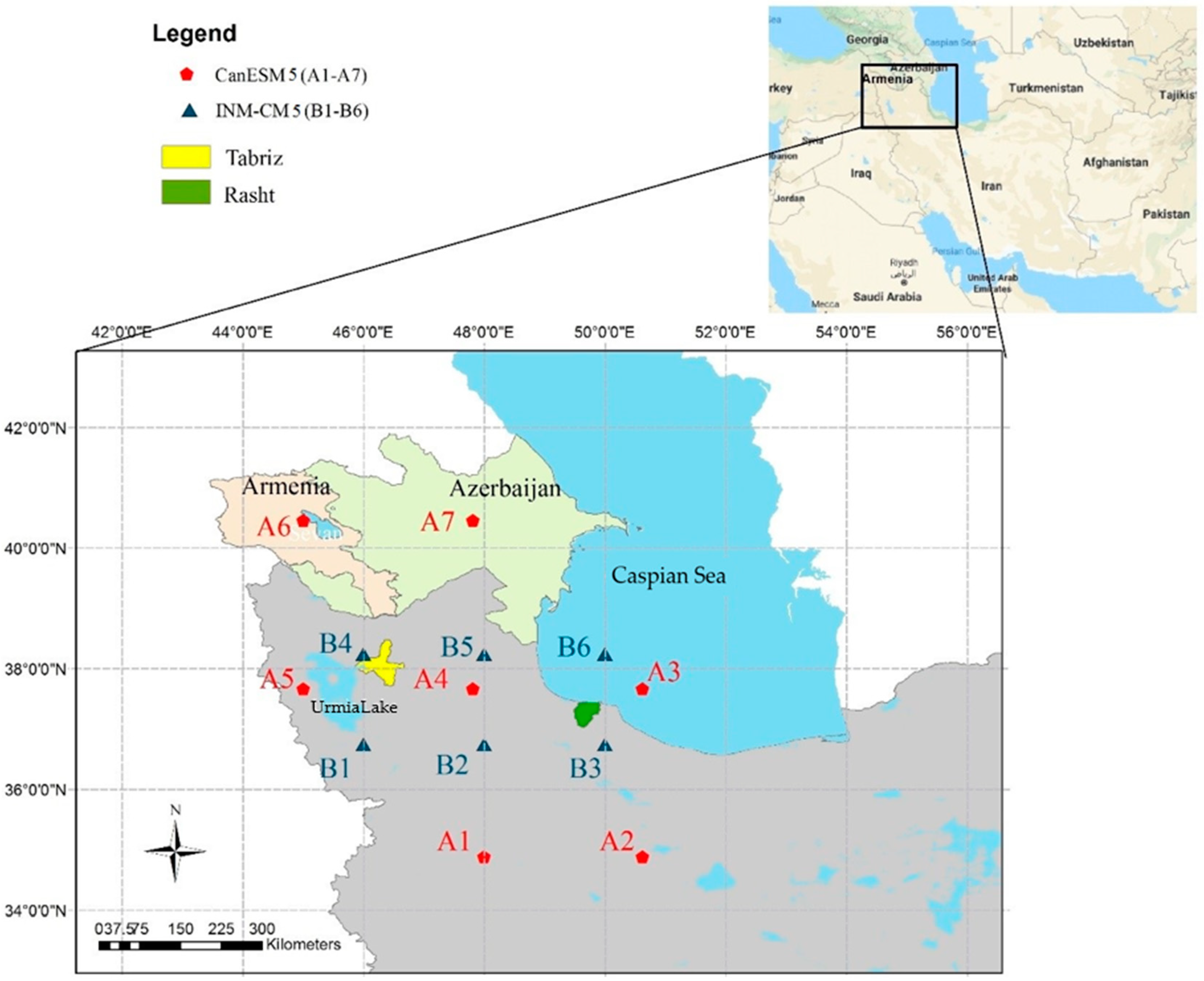
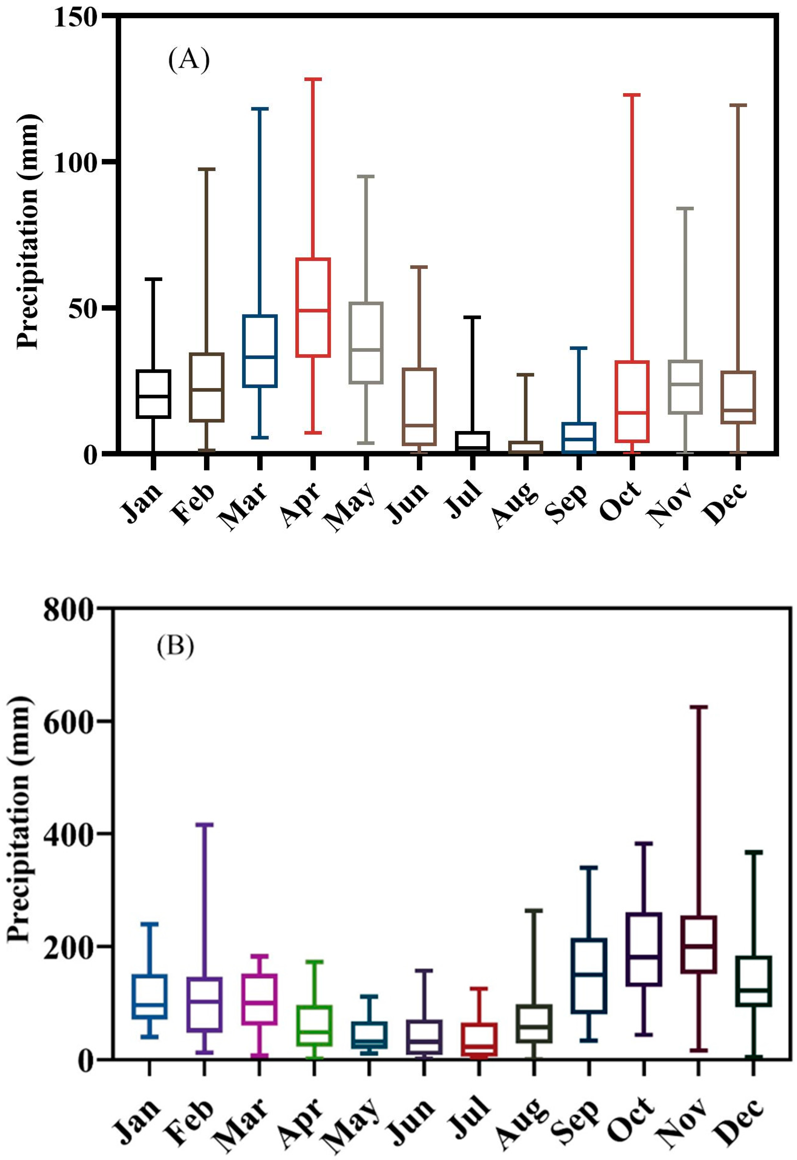
2.1. Study Area

The use of climate modeling and downscaling assists researchers in developing a better understanding of climate change, as well as quantifying its impacts, in various regions. The present study selected two study areas with different climate features, the attributes of which are described below.

In northwestern Iran, Tabriz City, the capital of East Azerbaijan province, is located on the western slope of the Tabriz plain, which ends at Urmia Lake (latitude 38.07° N, longitude 46.14° E). In the north is the Pakchin mountain, and in the east is the Payan mountain. The city’s southern boundary is formed of the Sahand mountain range. The city is positioned between 1350 and 1600 m above sea level. With regular seasons, Tabriz has a continental climate. Thus, the city has dry, semi-hot summers and cold, wet winters. Before the current decade, the city received 360 mm of precipitation per year on average, but this has decreased to 280 mm. January and July are the months with the lowest (−2 °C) and highest (19 °C) average temperatures in the city. The relative humidity varies from 73% to 48% on average in December and June.

The second case study is the capital of Gilan province in northern Iran. Rasht City is located in the central part of the Gilan plain at 37.26° N and 49.58° E (see Figure 1). Among the cities on the coast of the Caspian Sea, Rasht is the largest. Rasht lies in a flat area with an average elevation of 5 m above sea level. The Alborz range is located in the south, and Mount Dorfak (2733 m) is the nearest high mountain. With 81.2% average humidity, Rasht has both subtropical and Mediterranean climates. Rasht is one of Iran’s wettest regions. Due to its vicinity to the Caspian Sea, Rasht has warm summers and cold winters, occasionally accompanied by snow. There is an average annual precipitation of 1255.5 mm, and an average temperature of 25.35 °C in July and 6.35 °C in January.

2.2. Applied Data

Monthly precipitation time series provided by the Iran Meteorological Organization from 1951 to 2014 for Tabriz City and from 1993 to 2014 for Rasht City were used in this study. Figure 2 depicts the monthly precipitation distribution at both stations; Tabriz’s wet season occurs during April and October, indicating maximum precipitation fluctuations, while July is the driest month (Figure 2A).

Accordingly, for Rasht City, November and May are the months with the highest and lowest precipitation, respectively.

As part of the proposed downscaling method, the IPCC-AR6_CMIP6 datasets were applied for 63 years from 1951 to 2014, which reflect data under the IPCC Assessment Report 6 and Coupled Model Intercomparison Project. This study also utilized the Sixth Assessment Report (AR6) under Shared Socioeconomic Pathways (SSPs) for predictand projection (see https://esgf-node.llnl.gov/ (accessed on 19 August 2023)), of which SSP2 and SSP5 were used in this study. This study employed two CMs established by Canadian (i.e., CAN-ESM5) and Russian (i.e., INM-CM5) research centers (see

Table 1. Applied CMs.

Country	Center Acronym	Model	Grid Size	RCP (w/m2)	Applied Climate Variables in CM
Canada	CCCma 1	Can-ESM5	2.81 × 2.81	SSP2-4.5 SSP5-8.5	P ua: eastward wind P va: northward wind P zg: geopotential height P hur: relative humidity P hus: specific humidity tas: air temperature uas: eastward near-surface wind vas: northward near-surface wind psl: air pressure at sea level hfls surface upward latent heat flux prc: convective precipitation flux pr: precipitation flux hurs: near-surface relative humidity huss: near-surface specific humidity evspsbl: water evaporation flux
Russia	INM 2	INM-CM5	1.5 × 2	SSP2-4.5 SSP5-8.5

¹: Canadian Centre for Climate Modelling and Analysis. ²: Russian Academy of Sciences, Institute of Numerical Mathematics. ^P: 100 pa, 200 pa, 300 pa, 500 pa, 700 pa, 1000 pa, 2000 pa, 3000 pa, 5000 pa, 7000 pa, 10,000 pa, 15,000 pa, 20,000 pa, 30,000 pa, 40,000 pa, 50,000 pa, 60,000 pa, 70,000 pa, 85,000 pa, 92,500 pa, 100,000 pa.

).

According to the CM resolution, in the present study, predictors from four grid points were selected over the vicinity of the Tabriz and Rasht stations (Figure 1) for downscaling purposes [22,23]. Nevertheless, dominant predictors were identified later based on the proposed methodology. A1, A2, A3, A4, A5, A6, and A7 represent the four grid points considered for Can-ESM5, and B1, B2, B3, B4, B5, and B6 refer to the four grid points considered for INM-CM5.

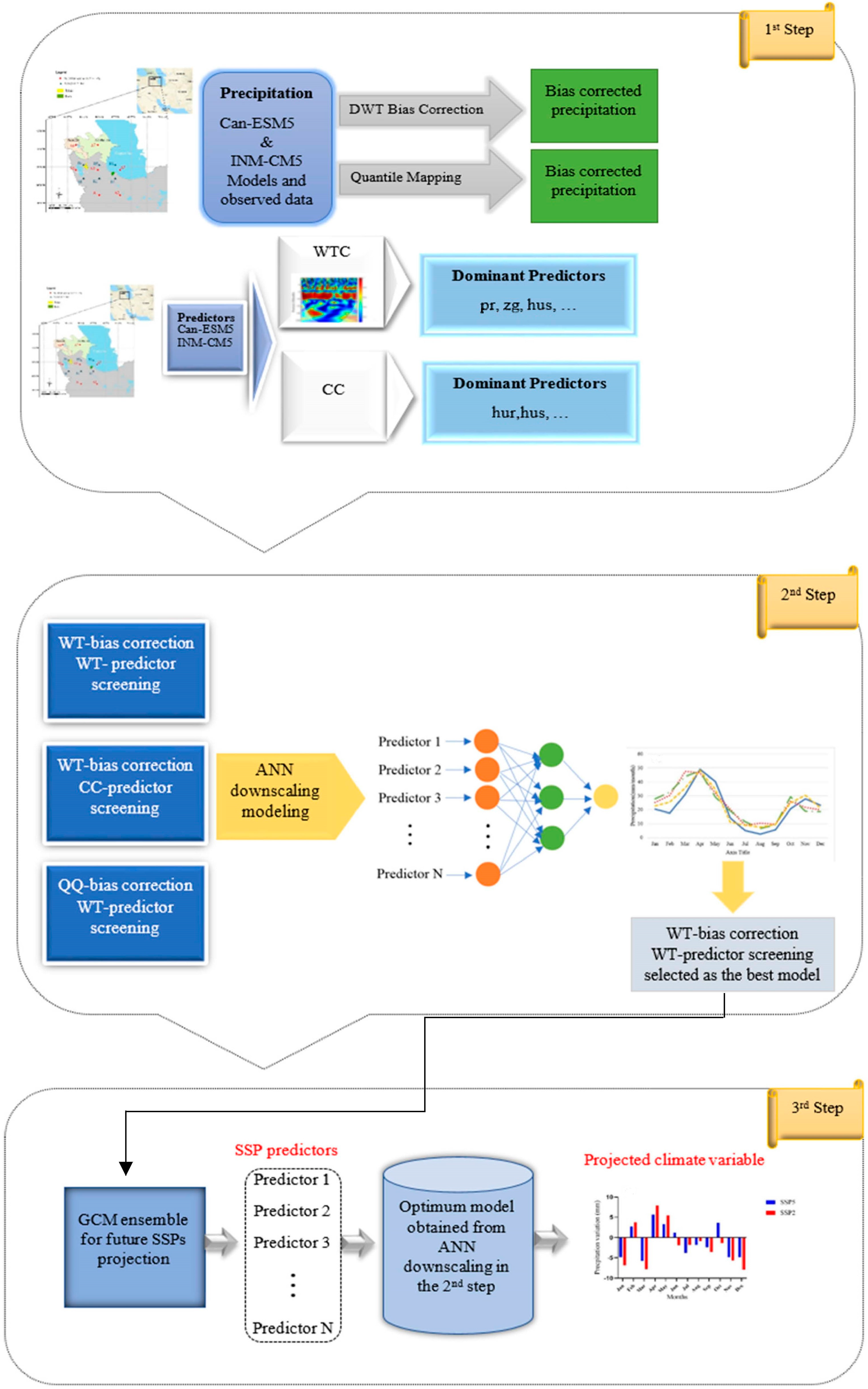
2.3. Proposed Methodology

This study aims to apply wavelet-based bias correction and predictor screening techniques to future precipitation projections for Tabriz and Rasht. An overview of the study is outlined in three steps in Figure 3.

In the first step, data pre-processing including bias correction and predictor screening was employed. The predictor and predictand time series in the baseline were split into detail subseries via DWT for bias calculation. Then, dominant variables were determined using the WTC predictor screening method. In the second step, the bias-corrected and screened dominant predictors were fed into the ANN-based downscaling model. After developing the model in the second step, the third step performed projections considering SSP2 and SSP5. Detailed descriptions of the methodology are provided below:

2.3.1. First Step

In this step, bias correction and data screening methods were applied using DWT and WTC, respectively. To this end, the predictor and predictand datasets were divided into two equal time series. For the Tabriz station, the datasets were separated into 1952–1978 and 1979–2005. Similarly, for the Rasht station, the time series were split into 1993–2003 and 2004–2014. Predictor time series were decomposed into detail subseries, and the difference between each decomposed time series of predictor and predictand was calculated by subtracting each of the similar details from each other. The bias-corrected time series were then derived by adding the computed differences to the second half of the baseline datasets. Furthermore, the results were compared with the QM technique to evaluate the performance of the proposed method.

Next, the dominant periodicity and coherence for observed precipitation and predictors (including bias-corrected precipitations obtained from the first step) were estimated via WTC. This could provide detailed information about the linear and nonlinear relationships between predictors and predictands. Thereafter, the coherence value between large-scale CM variables and local station data was estimated by calculating the Scale Average Coherency (SAC). To this end, a matrix of significant scales with a confidence level of 95 percent was calculated for the coherency of the wavelet to assess the influence of each large-scale variable. Then, the results were compared with the linear CC method.

The INM-CM5 data from the applied grid points included 95 predictors without using any data pre-processing techniques, and the Can-ESM5 included 120 variables. Thus, 2^k − 1 variables should be applied in the downscaling process, which is time-consuming. Finally, ANN-based downscaling was performed using the dominant predictors derived from the WTC and CC methods.

2.3.2. Second Step

Based on the dominant parameters obtained in step one, ANN was used to implement a statistical downscaling model by feeding selected variables from the WTC and CC methods and bias-corrected predictors from the QM and DWT methods into the ANN model. Moreover, to compare the results of the developed model, a statistical downscaling model (SDSM) was implemented to downscale the selected CM parameters. Consequently, the performance of the methods was examined by considering three evaluation criteria. As a statistical measure, the CC measures how strongly two variables are related, as defined by [37]. During the training and validation phases, the Root Mean Square Error (RMSE) and Determination Coefficient (DC) were used to assess the performance of the proposed methodology. According to [38,39,40], these two criteria are sufficient to evaluate hydro-climatology studies for prediction purposes.

2.3.3. Third Step

The SSP2 and SSP5 values from CMIP6 were used to project future precipitation based on the best model developed in the earlier step. Since anthropogenic effects such as population growth, greenhouse gas emissions, and economic conditions influence the environment from diverse perspectives, there are different radiative forcing pathways associated with each SSP. Accordingly, SSP2 corresponds to moderate-emission scenarios, while SSP5 corresponds to high-emission scenarios.

The following sections provide an overview of the mathematical methods used in the proposed methodology:

2.4. Wavelet Analysis

WT is an acclaimed mathematical transform widely used for processing images and signals. There are intermittent characteristics of many climatic phenomena in terms of their spatial and temporal dimensions; it is possible to identify those features via other domains like frequency. In this way, wavelet transform offers an improved method for analyzing time series in terms of time and scale. Based on [41], the CWT of a time series like $x\left(t\right)$ is:

$$T\left(a,b\right)=\frac{1}{\sqrt{a}}{\int }_{+\infty }^{-\infty }x\left(t\right){\Psi }^{*}(\frac{t-b}{a})dt;a,b\in R$$

(1)

$\Psi$ represents the mother wavelet, $*$ represents the complex conjugate of the wavelet function, $a$ represents the scale factor, and $b$ represents the time-related translation magnitude. Mother wavelets present continuous translated and dilated wavelets as their primary function.

It has been found that decomposing a subseries via CWT is computationally expensive and complex in practice. DWT-based signal decomposition considering the powers of two was devised in response to this issue. According to [41], the DWT consists of the following components:

$${\Psi }_{\left(j,k\right)}\left(t\right)=\frac{1}{\sqrt{{a_0}^k}}\Psi \left(\frac{t-k\times b_0{a}_0^j}{a_0^j}\right)$$

(2)

where $\Psi$ is the mother wavelet, and $j$ and $k$ are scaling and transform parameters, respectively.

With DWT, a signal is decomposed and rebuilt through filters. To construct an approximation and detail time series, high-pass and low-pass filters are used to pass the main signal through them. As an outline, the approximate signal represents the low-frequency portion of the main signal, while the details provide high-frequency information. The decomposition process is repeated by decomposing the approximation signal into new approximations and detail signals. The main signal will ultimately result from a fusion of an approximation signal and a couple of details. In the present study, Daubechies mother wavelets with four vanishing moments (db4) resemble hydroclimatological time series. Thus, for applying DWT, db4 was employed.

CWT can detect the correlation between two variables [42], where Torrence and Compo formulate the wavelet spectrum of a continuous signal $X\left(t\right)$ as follows [43]:

$$W_X\left(a,b\right)=C_{\Psi }^X\left(a,b\right)C_{\Psi }^{*X}\left(a,b\right)=|{C_X\left(a,b\right)|}^2$$

(3)

where $C_{\Psi }^X\left(a,b\right)$ and $C_{\Psi }^{*Y}\left(a,b\right)$ are the respective coefficients of continuous wavelets and conjugates of X(t). In order to detect the cross wavelet power, phase relationships, and fluctuations that occur between two time series $X\left(t\right)$ and $Y\left(t\right)$, we can visualize the cross-wavelet spectrum as follows [44]:

$$W_{XY}\left(a,b\right)=C_{\Psi }^X\left(a,b\right)C_{\Psi }^{*Y}\left(a,b\right)$$

(4)

In this case, $C_{\Psi }^X\left(a,b\right)$ is the continuous wavelet spectrum of $X\left(t\right)$, while $C_{\Psi }^{*Y}\left(a,b\right)$ is the complex conjugate of $Y\left(t\right)$. Despite the limited capability of identifying relationships between signals, which was pointed out by Maraun and Kurths and Ng and Chan, we described the complex cross-wavelet spectrum formula as [32,35]:

$$W_{XY}\left(a,b\right)=\left|W_{XY}\left(a,b\right)\right|e^{i{\phi }_{is}}$$

(5)

where ${\phi }_{is}$ is the phase distinction among two signals at the scale $s$ and the time $t_i$. As stated before, XWT has limitations in analyzing the local-scale correlation. The localized correlation among the time series is named WTC, which is a powerful tool for identifying the time–frequency relationship between two time series [45]:

$$WC(a,b)=\frac{\left|{SW}_{XY}\left(a.b\right)\right|}{\sqrt{\left|{SW}_{XX}\left(a.b\right)\right|.\left|{SW}_{YY}\left(a.b\right)\right|}}$$

(6)

where ${SW}_{XY}\left(a.b\right)$, ${SW}_{YY}\left(a.b\right),\mathrm{a}\mathrm{n}\mathrm{d}{SW}_{XX}\left(a.b\right)$ are the flat estimations of the cross-wavelet spectrum relevant to the $X\left(t\right)$ and $Y\left(t\right)$ signals, and $X\left(t\right)$ and $Y\left(t\right)$ time series, respectively [45]:

$${SW}_{XX}\left(a.b\right)={\int }_{t-\frac{\delta }{2}}^{t+\frac{\delta }{2}}{W}_{XX}^{*}\left(a.b\right)W_{XX}\left(a.b\right)dadb$$

(7)

$${SW}_{yy}\left(a.b\right)={\int }_{t-\frac{\delta }{2}}^{t+\frac{\delta }{2}}{W}_{yy}^{*}\left(a.b\right)W_{yy}\left(a.b\right)dadb$$

(8)

$${SW}_{XY}\left(a.b\right)={\int }_{t-\frac{\delta }{2}}^{t+\frac{\delta }{2}}{W}_{XX}^{*}\left(a.b\right)W_{YY}\left(a.b\right)dadb$$

(9)

In this study, WTC was performed using Morlet mother wavelets since it has shown the most effectiveness in localizing time and frequency in non-stationary signals [34].

2.5. Quantile Mapping (QM)

The quantile mapping method matches the CDFs of two time series based on their distributions. Generally, QM is described as follows [46]:

$$P_q=F_o^{-1}\left(F_m\right(P_m\left)\right)$$

(10)

where $F_m$ represents the CDF of simulated data of the CM, and $P_m$ shows the simulated data. $P_q$ identifies the transformed variable following quantile mapping, and $F_o^{-1}$ corresponds to the inverse CDF of the observation values. This study implemented QM using the QUANT method. The empirical CDF of the model and observed variables could be calculated using QUANT. More details of the QM methods are discussed in [46].

2.6. Artificial Neural Network (ANN)

Modeling non-linear time series using ANN has demonstrated acceptable performance in a wide range of applications. Basic ANN structures consist of three layers containing inputs, hidden layers, and outputs. A training dataset is imported into an input layer, and relevant results are generated based on the input dataset. ANN consists of layers of neurons connected within each layer. A typical ANN structure can be described as follows [47]:

$${\widehat{y}}_k=f_0\left[{\sum }_{j=1}^{M_N}{w}_{kj}.f_h\left({\sum }_{i=1}^{N_N}{w}_{ji}{x}_i+w_{j0}\right)+w_{k0}\right]$$

(11)

Input, hidden, and output neurons are represented by $i$, $j$, and $k$, respectively. Each input and output layer consists of $N_N$ and $M_N$ neurons. The hidden neuron and the output layer are activated by $f_h$ and $f_0$, respectively. The input layer’s weight is $w_{ji}$, and its bias is $w_{j0}$. The hidden layer’s weight is $w_{kj}$, and the $k_{th}$ output neuron’s bias is $w_{k0}$. $x_i$ is the input to the $i_{th}$ input layer, and ${\widehat{y}}_k$ is the associated output. In the present study, a three-layer Feed-Forward Network (FFNN) with a Back Propagation (BP) algorithm was used due to previous studies showing its effectiveness [48]. Furthermore, tangent Sigmoids and the Levenberg–Marquardt schemes were used at the training stage to improve the ANN’s performance [47].

In order to determine the optimal number of hidden layer neurons and epochs, a trial-and-error approach was taken. For this case, the optimum structure consisted of 410 epochs and 5 neurons.

3. Results and Discussion

The current research employed wavelet-based bias correction and predictor screening pre-processing methods to downscale and project future precipitation for the Tabriz and Rasht stations for the future. The results of study are explained based on the steps presented in the Section 2:

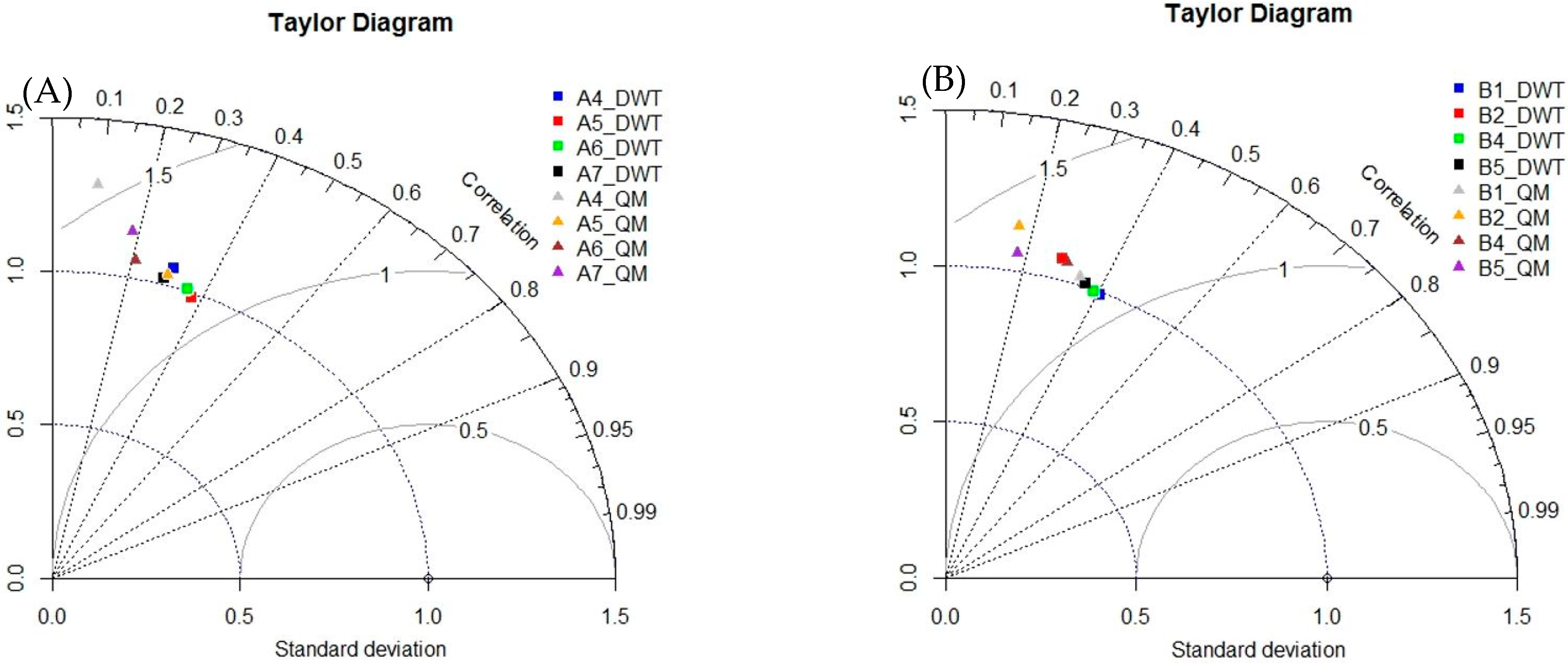
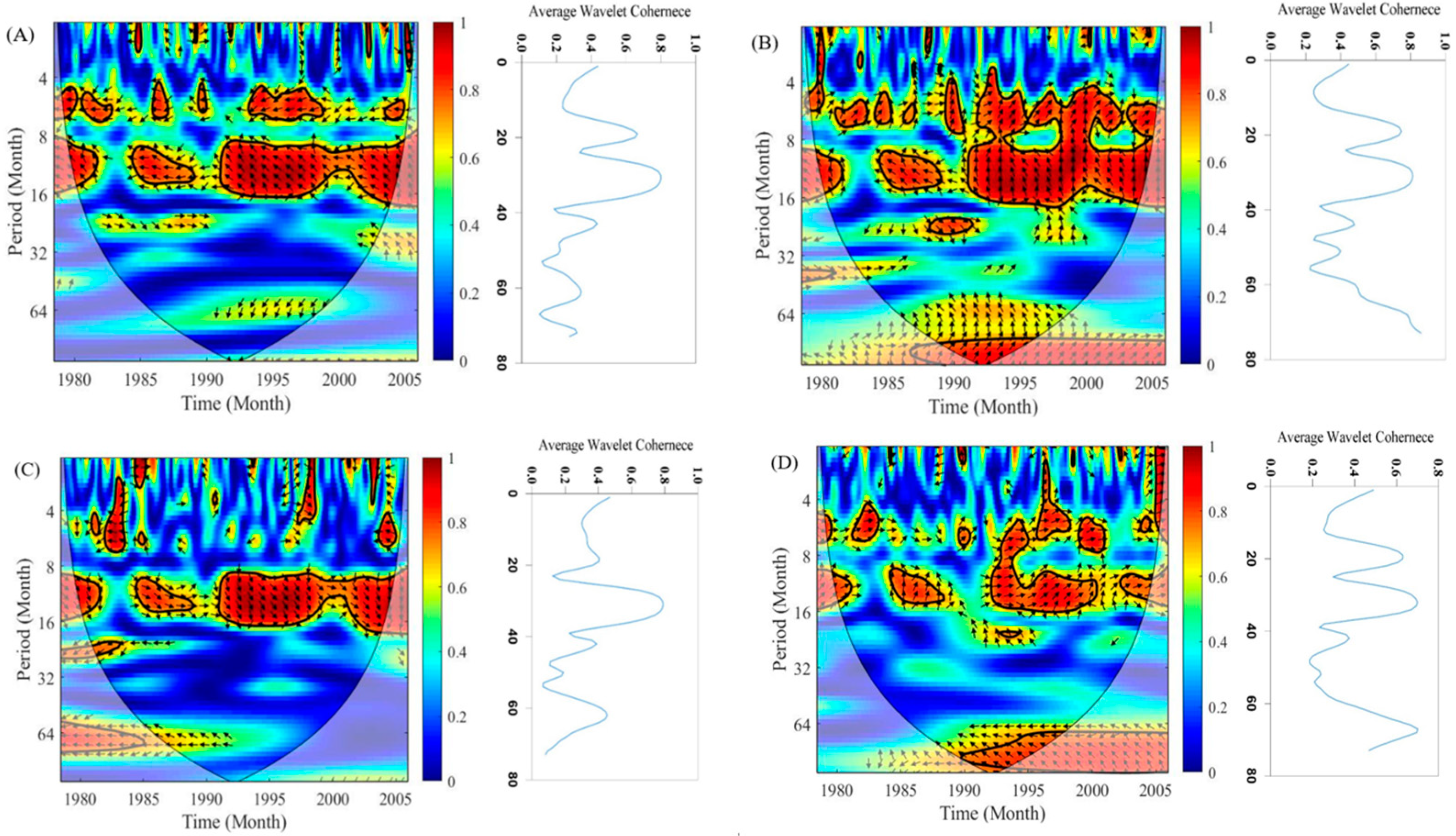
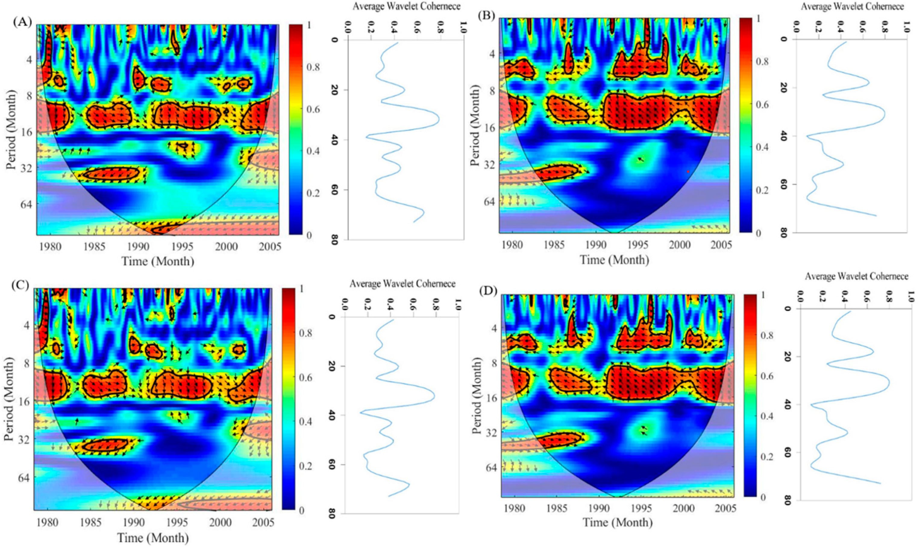
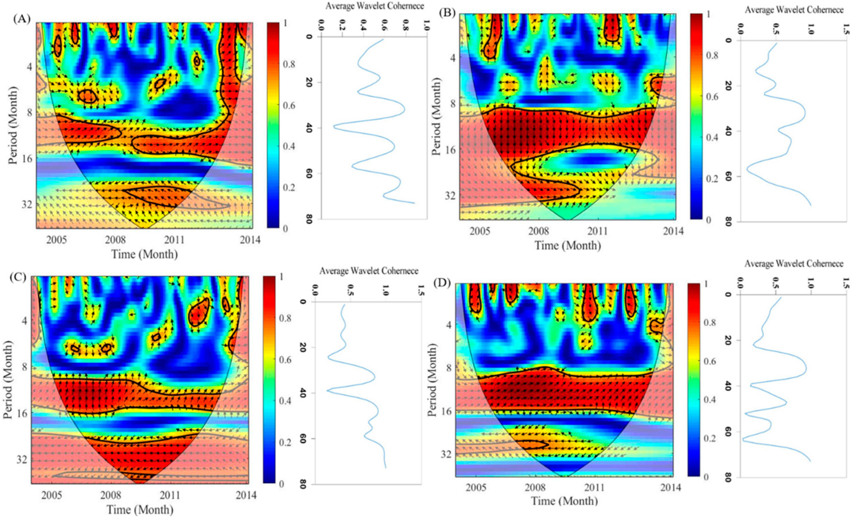
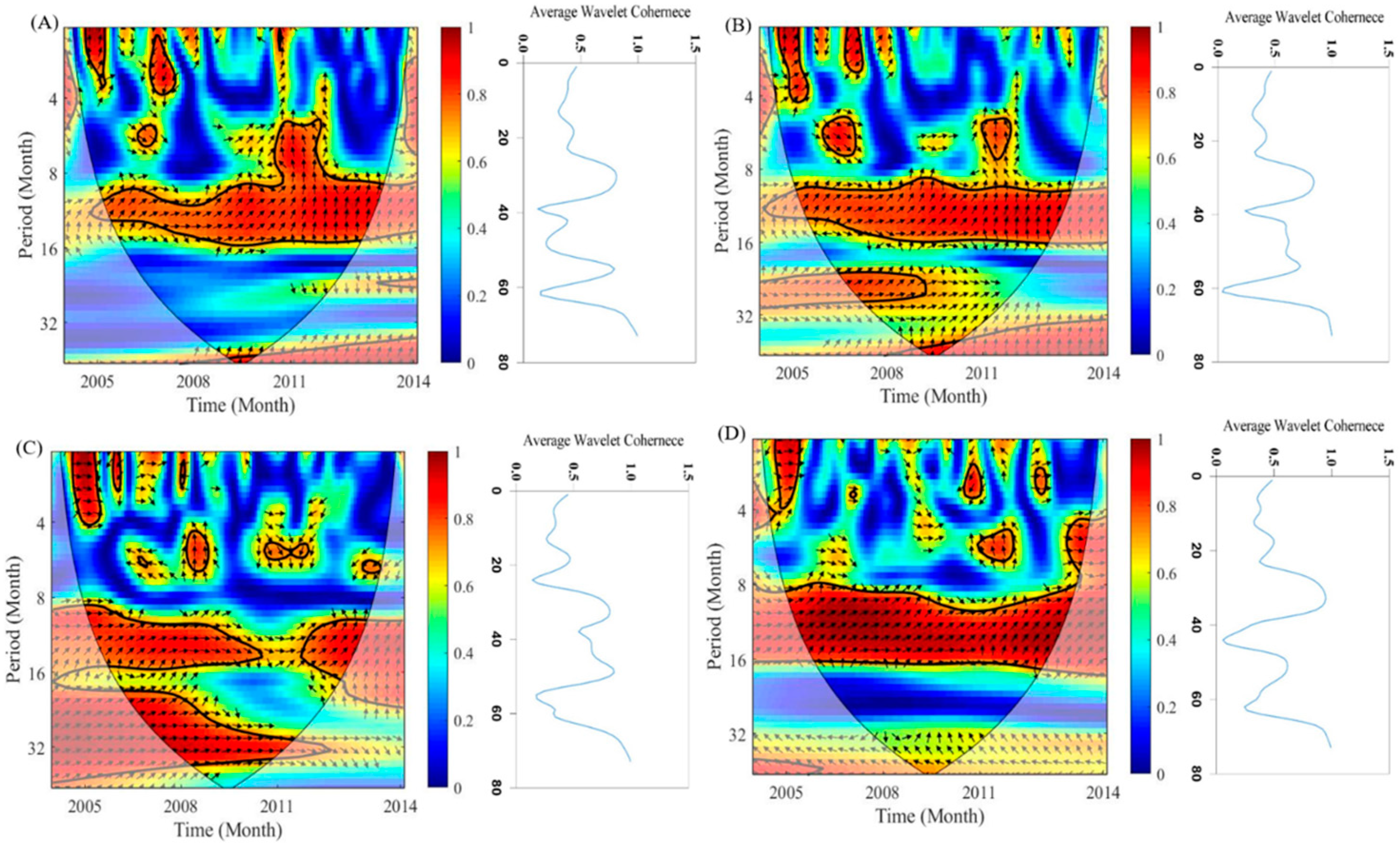
3.1. First Step—Bias Correction and Predictor Screening via WT

Firstly, the historical datasets were separated into two parts. Part one applied the bias correction technique, and the subsequent part evaluated the bias-corrected model. In this regard, the historical and model data from Tabriz were segmented into the 1951–1978 and 1979–2014 periods, and the data of the Rasht station were segmented into the 1993–2003 and 2004–2014 periods. Approximation and detail subsets were decomposed for each city. All the corresponding decomposed wavelets in the first part of the predictors (i.e., 1951–1978 and 1993–2003) were subtracted from the corresponding predictands. In order to obtain the bias-corrected output, the subtracted values were added to the second part of the decomposed predictor. Figure 4 and Figure 5 demonstrate the results of the DWT and QM methods for the Tabriz and Rasht stations, respectively. As shown in Figure 4A, the bias correction based on the DWT method performs better at grid points A6 and A5 for the Tabriz station than at other grid points. Figure 4B shows that the DWT bias correction method at grid points B1 and B4 stands out among the other grid points for the Tabriz station.

According to Figure 5A, for Rasht City, the DWT-based bias correction method performs better at grid points A3 and A4 in removing the bias of Can-ESM5. As can be seen in Figure 5B, the DWT method eliminated bias in the INM-CM5 at grid points B5 and B6 more accurately. Considering the results of the bias correction methods, it appears that the proposed DWT method performs better than QM, since WT can identify dominant periodicities in non-stationary signals. The QM method, however, merely adjusts the CDF of the two signals.

Wavelet-based predictor screening between predictors and predictands was conducted using the WTC method, where the SA coherency or the energy of coherency was assessed, to determine the dominant predictors. The WTC values led to a significant values matrix with a 95% confidence level, and were then ranked by SA wavelet coherency. Consequently, the maximum SA values were selected as predominant predictors.

To determine the most influential predictors, the linear relationships between the predictors and station data were computed in terms of CC. The maximum CC value was evaluated; then, the corresponding predictors were identified, and CC values over 0.3 were considered acceptable. According to data screening results tabulated in

Table 2. Predictors selected according to linear CC and nonlinear WTC methods.

	Selected Predictors for Tabriz (i)		Selected Predictors for Rasht (i)
CM	WTC	CC	WTC	CC
CAN-ESM5	zg20000 (4) hus (5) BCP (5) BCP (6)	hur7000 (4) hur10000 (4) BCP (5) hus7000 (5)	BCP (3) hur7000 (3) BCP (4) hus100 (4)	zg85000 (1) zg85000 (2) BCP (4) zg925000 (4)
INM-CM5	BCP (1) BCP (4) zg15000 (4) zg15000 (5)	BCP (1) hur15000 (2) BCP (4) hur20000 (5)	BCP (5) BCP (6) hus60000 (6) ua100 (6)	zg92500 (3) BCP (6) zg92500 (6) hfls (6)

⁽ⁱ⁾ The grid points surrounding the study area are numbered as i = 1,2,3,4.

, the dominant predictors from the CC method were relative to the specific humidity at various pressure levels for the Tabriz station. However, for the Rasht station, the dominant predictors were relevant to geopotential and hfls. Moreover, bias-corrected precipitation (BCP) was selected from both stations as the dominant predictor with a linear relationship with local precipitation.

Based on the linear relationship between humidity and regional precipitation, at the grid points A4, A5, A6, B1, B4, and B5, humid resources such as Lake Urmia, the Caspian Sea, and Lake Sevan, which are in the vicinity of the study areas, are highly influential (see Figure 1).

Compared to the CC method for the Tabriz station, the WTC method’s representative predictors were BCP, geopotential height (zg), and specific humidity (hus), where zg was different from the CC-based prominent predictors. However, for the Rasht station, the WTC-based predictors were BCP, hu, and ua, which were also different from the linear CC-based selectees. Due to the capability of WT to cope with non-stationary time series, the obtained dominant variables imply that WTC can identify variables with both linear and non-linear relationships between precipitation and CM outputs. For both stations, Figure 6, Figure 7, Figure 8, Figure 9 and Figure 10 show the WTCs between the dominant predictors and predictands. It should be noted that in these figures, the relative phase relationship is shown as arrows, where the in-phase status points right, the anti-phase status points left, a value of 1 with a red color indicates high coherence, and a value of 0 with a blue color indicates no coherence. Figure 6 illustrates the WTC between the precipitation of Tabriz City and Can-ESM5 predictors, where there are in-phase and anti-phase relationships between the predictors and predictand. For instance, there is anti-phase coherence between precipitation and zg20000 in the 4–8 and 8–16-month periods (Figure 6A). It is noted that in all figures relevant to the WTC illustration of the predictors and predictand, the thick black lines surrounding the red parts indicates a confidence level of 95%, and the lighter shade around the impact cone depicts the edge effect’s influence on the calculations. Figure 7 illustrates the WTC between precipitation and the influencing parameters of INM-CM5 for the Tabriz station, where precipitation has an in-phase coherence with BCP at an 8–16-month periodicity (Figure 7A) and an anti-phase relationship with zg15000 at the 4–8 and 8–16-month signals (Figure 7B).

At all four grid points used for downscaling the precipitation of Rasht City, geopotential height, BCP, and surface upward latent heat flux (hfls) were found to be the dominant predictors according to the CC method. In Table 2, the dominant predictors include hur, hus, and eastward wind (ua), determined by their coherence values between precipitation variables. Figure 8 shows the WTC among the CAN-ESM5 predictors and predictand precipitation with significant in-phase coherence between the precipitation and dominant variables at the 8–16-month signal. Similarly, the predominant predictors for INM-CM5 CM are depicted in Figure 9, where precipitation has in-phase coherence with the BCP and hus predictors at 8–16 months. Using the WTC method, it can be concluded that zg, precipitation, and humidity have the most significant influence on Tabriz’s precipitation. Rasht City’s precipitation, however, appears to be heavily influenced by humidity. This could be rooted in the distinct climate and geographical attributes of the two cities, where because of the mountain range around Tabriz City, the geopotential can affect precipitation nonlinearly, and humidity in upper levels of the atmosphere impacts linearly, whereas for Rasht City, being in the vicinity of the Caspian Sea, the humidity parameter becomes dominant.

3.2. Second Step—ANN-Based Statistical Downscaling

First, all the data were standardized in advance to remove the effects of various units and to make them comparable. Approximately three-fourths (75%) of the potential inputs, as well as observed data, was used for calibration, and one-fourth (25%) was used for validation. According to prior studies [49], such data partitioning is effective for modeling hydrological processes. The ANN downscaling approach was applied to different types of predictors that were bias-corrected using the DWT and QM methods: (i) dominant predictors selected based on the WTC method, (ii) dominant predictors selected according to their linear relationship via CC, and (iii) downscaling via SDSM. To examine the effectiveness of wavelet-based bias correction and data screening on downscaling the precipitation of the Tabriz and Rasht stations (see

Table 3. The performance of ANN-based downscaling methods based on various predictor screening and bias correction methods along with SDSM downscaling performance.

Station	Bias Correction Method	Predictor Screening Method	Model	RMSE Train (mm)	RMSE Verification (mm)	DC Train	DC Verification
Tabriz	DWT	WTC	WT-ANN	22	24	0.617	0.614
		CC	WT-CC-ANN	29	30	0.519	0.444
	QM	WTC	QM-ANN	27	30	0.411	0.351
		CC	QM-CC-ANN	30	32	0.476	0.391
	-	-	SDSM	33	35	0.342	0.318
Rasht	DWT	WTC	WT-ANN	32	32	0.589	0.579
		CC	WT-CC-ANN	43	47	0.441	0.426
	QM	WTC	QM-ANN	38	52	0.474	0.344
		CC	QM-CC-ANN	41	42	0.433	0.432
	-	-	SDSM	43	46	0.392	0.371

), each bundle of datasets was considered separately as inputs for ANN statistical downscaling. According to the results, WT bias correction and WTC feature extraction are superior to the CC and QM methods. In this study, a more comprehensive assessment of local climate variables depends on WT’s ability to cope with the non-stationary and nonlinear features of climate data, since the QM method utilizes only four sections of distribution to match the time series, although data distribution could not be same. In contrast, the QM method relies solely on the matching of four distribution sections to time series data. Furthermore, the data distributions may not align perfectly, yet the QM method still treats them as similar. ANN downscaling using WT, therefore, provides more accurate future climate predictions. According to the DC, the WT-ANN approach performs 17–26% better than the other two methods for Tabriz precipitation downscaling. Additionally, for Rasht precipitation, the downscaling results based on the WT-ANN method show that it is superior to the CC-based and QM-based methods, as 15.3–23.5% efficiency was calculated for DC validation. According to Figure 10, the downscaling results indicate that WT-ANN outperforms both the QM and CC downscaling methods for both stations. Furthermore, Figure 10A shows the accuracy of the WTC-ANN downscaling method in simulating the precipitation value in April for Tabriz City, while for Rasht City, the WT-ANN shows the exact simulation in March. In addition, Tabriz City’s ANN downscaling for precipitation shows better performance compared to Rasht City. As a result, one CM might yield different results at different stations due to the various atmospheres and locations and complex factors affecting precipitation.

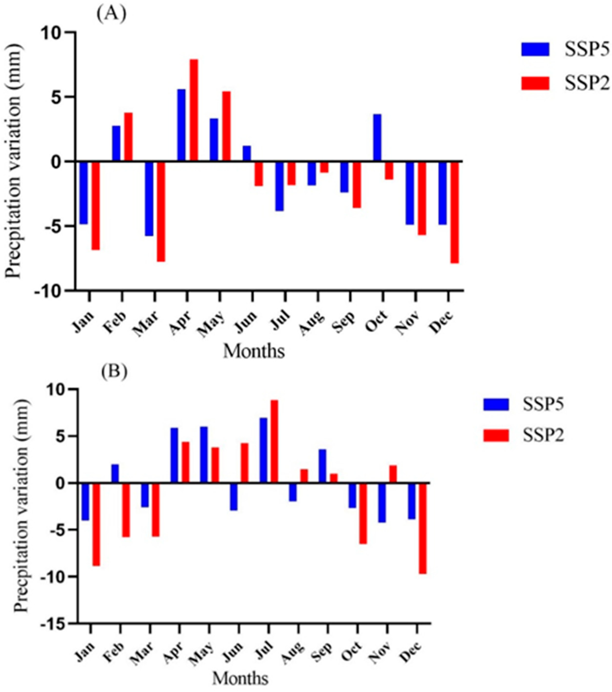
3.3. Third Step—Precipitation Projection

As a final step, two CMs (i.e., Can-ESM5 and INM-CM5) were applied to predict future variations under the SSP2 and SSP5 scenarios using the ANN optimal downscaling model (i.e., DWT-based bias correction and WTC-based predictor screening).

Due to the greater accuracy obtained from WTC-based predictor screening, future precipitation projections were made in Tabriz and Rasht based on the dominant variables determined at each station.

The ANN projection models were developed using predictors from the Can-ESM5 and INM-CM5 models. For verifying the ANN results with the predictands, the difference between projected monthly precipitation and observations during the historical period was calculated for each month, as shown in Figure 11. The figure illustrates both rises and falls in seasonal future precipitation for both study areas. Concerning the average annual period, future precipitation is predicted to decrease significantly in the model under the SSP2 scenario, with a value of 6.1%. A 3.4% decrease in precipitation is also predicted by the WT-ANN model for Tabriz City under the SSP5 scenario.

Considering the presented figure for Tabriz City (see Figure 11A), it is clear that this city will undergo a substantial reduction in precipitation during the winter, summer, and fall seasons. Conversely, there is a notable alteration in the precipitation pattern during the spring, potentially leading to a heightened risk of flooding during this period. Consequently, the regional water management authorities should take cognizance of this declining trend, as it can exert a profound impact on agricultural activities during winter and fall. Furthermore, these authorities must remain vigilant and well prepared during the spring season.

During winter and fall, Rasht City will experience an increase in precipitation. However, in spring and summer, precipitation will decrease (Figure 11B). In areas near the sea, such as Rasht City, increasing water vapor in the atmosphere is the major reason for increased precipitation during winter and fall. According to the WT-ANN model, precipitation is expected to decline by 2.5% under the SSP2 scenario. Under SSP5, however, Rasht City’s monthly precipitation variation drops by 1.5%. The maximum decrease and increase are 13 and 9 mm, respectively. Overall, precipitation will decrease despite seasonal fluctuations. Moreover, there will be more extreme weather events in these study regions. Similarly, the IPCC report indicated that “the rate of heavy precipitation and heatwaves will increase in majority of earth specifically Asia” [50].

The primary objective of this study is to evaluate a developed methodology across diverse regions, where each model’s performance is assessed based on its historical data. This assessment encompasses not only a comparison of reliability between two regions, but also an examination of the methodology’s suitability for each region independently. Furthermore, it is crucial to note that the study area is situated within a developing country characterized by a limited database of historical hydrological data. In such a context, the adoption of a uniform data duration for research in developing countries would impede the initiation of any meaningful research endeavors.

4. Conclusions

The purpose of this study was to determine the impact of the developed WT-based bias correction and predictor screening methods on enhancing downscaling performance to assess and project the impact of climate change on precipitation variations at the Tabriz and Rasht synoptic stations over the period of 2021–2060. Therefore, the monthly observed precipitation of Tabriz and Rasht, as well as the Can-ESM5 and INM-CM data, were fed to the developed ANN model. CM variables are associated with systemic biases, so a wavelet-based bias correction method was proposed. In comparison to the common QM method, the wavelet-based method demonstrated more improvement. The climate in an area is affected by a variety of predictors, but not all variables have equal impacts, as some predictors correlate strongly with predictands, while others do not. For this reason, selecting essential variables as inputs to the ANN downscaling model is vital so as to avoid redundancy in the input matrix. Based on the ANN downscaling model results, the WT-based bias correction and predictor screening approach was superior to the CC-driven and QM-based methods, respectively, due to their ability to identify the relationships between predictors and predictands, as well as coping with non-stationary signals by considering the multi-resolution effect. Compared to the CC-based and QM-based methods, WT-ANN statistical downscaling improved Tabriz precipitation modeling by 17–26% and Rasht precipitation modeling by 15.3–23.5%. The results showed that Tabriz’s precipitation will decrease by 3.4% to 6.1%, while Rasht’s precipitation will decrease by 1.5% to 2.5%. While rising GHG emissions will increase global warming, precipitation trends will not follow a similar pattern across regions.

In light of these results, it is advisable for authorities to reconsider regulations related to agricultural practices and water management systems, which heavily rely on precipitation patterns. To further enhance the robustness of such studies, it is recommended to incorporate a diverse range of climate models and scenarios to account for uncertainties. Increased precision can be achieved by conducting multiple model runs, and alternative bias correction methods, such as SOM clustering or Decision Trees, can be explored and compared with the WTC method. As ANN has a straightforward structure and is precise, it was used in this study to downscale data. However, other models such as SVR, SVM, and deep learning methods, which are AI models, can help to identify the strengths and weaknesses of different models when downscaling climate variables.

References

1. Wilby, R.; Wigley, T. Downscaling general circulation model output: A review of methods and limitations. Prog. Phys. Geogr. Earth Environ. 1997, 21, 530–548. [Google Scholar] [CrossRef]
2. Timbal, B.; Dufour, A.; McAvaney, B. An estimate of future climate change for western France using a statistical downscaling technique. Clim. Dyn. 2003, 20, 807–823. [Google Scholar] [CrossRef]
3. Pahlavan, H.A.; Zahraie, B.; Nasseri, M.; Varnousfaderani, A.M. Improvement of multiple linear regression method for statistical downscaling of monthly precipitation. Int. J. Environ. Sci. Technol. 2017, 15, 1897–1912. [Google Scholar] [CrossRef]
4. Mohammad, N.; Moradkhani, H.; Susan, A.W. Statistical Downscaling of Precipitation Using Machine Learning with Optimal Predictor Selection. J. Hydrol. Eng. 2011, 16, 650–664. [Google Scholar]
5. Sun, L.; Lan, Y. Statistical downscaling of daily temperature and precipitation over China using deep learning neural models: Localization and comparison with other methods. Int. J. Clim. 2020, 41, 1128–1147. [Google Scholar] [CrossRef]
6. Hoai, N.D.; Udo, K.; Mano, A. Downscaling Global Weather Forecast Outputs Using ANN for Flood Prediction. J. Appl. Math. 2011, 2011, 246286. [Google Scholar]
7. Harpham, C.; Wilby, R.L. Multi-site downscaling of heavy daily precipitation occurrence and amounts. J. Hydrol. 2005, 312, 235–255. [Google Scholar] [CrossRef]
8. Tisseuil, C.; Vrac, M.; Lek, S.; Wade, A.J. Statistical downscaling of river flows. J. Hydrol. 2010, 385, 279–291. [Google Scholar] [CrossRef]
9. Chadwick, R.; Coppola, E.; Giorgi, F. An artificial neural network technique for downscaling GCM outputs to RCM spatial scale. Nonlinear Process. Geophys. 2011, 18, 1013–1028. [Google Scholar] [CrossRef]
10. Su, B.; Zeng, X.; Zhai, J.; Wang, Y.; Li, X. Projected precipitation and streamflow under SRES and RCP emission scenarios in the Songhuajiang River basin, China. Quat. Int. 2015, 380–381, 95–105. [Google Scholar] [CrossRef]
11. Alotaibi, K.; Ghumman, A.R.; Haider, H.; Ghazaw, Y.M.; Shafiquzzaman, M. Future Predictions of Rainfall and Temperature Using GCM and ANN for Arid Regions: A Case Study for the Qassim Region, Saudi Arabia. Water 2018, 10, 1260. [Google Scholar] [CrossRef]
12. Prathom, C.; Champrasert, P. General Circulation Model Downscaling Using Interpolation—Machine Learning Model Combination—Case Study: Thailand. Sustainability 2023, 15, 9668. [Google Scholar] [CrossRef]
13. Teutschbein, C.; Seibert, J. Bias correction of regional climate model simulations for hydrological climate-change impact studies: Review and evaluation of different methods. J. Hydrol. 2012, 456–457, 12–29. [Google Scholar] [CrossRef]
14. Feyissa, T.A.; Demissie, T.A.; Saathoff, F.; Gebissa, A. Evaluation of General Circulation Models CMIP6 Performance and Future Climate Change over the Omo River Basin, Ethiopia. Sustainability 2023, 15, 6507. [Google Scholar] [CrossRef]
15. Eden, J.M.; Widmann, M.; Grawe, D.; Rast, S. Skill, Correction, and Downscaling of GCM-Simulated Precipitation. J. Clim. 2012, 25, 3970–3984. [Google Scholar] [CrossRef]
16. Watanabe, S.; Kanae, S.; Seto, S.; Yeh, P.J.-F.; Hirabayashi, Y.; Oki, T. Intercomparison of bias-correction methods for monthly temperature and precipitation simulated by multiple climate models. J. Geophys. Res. Atmos. 2012, 117, 127261. [Google Scholar] [CrossRef]
17. Cayan, D.R.; Maurer, E.P.; Dettinger, M.D.; Tyree, M.; Hayhoe, K. Climate change scenarios for the California region. Clim. Chang. 2008, 87, 21–42. [Google Scholar] [CrossRef]
18. Rajczak, J.; Kotlarski, S.; Schär, C. Does Quantile Mapping of Simulated Precipitation Correct for Biases in Transition Probabilities and Spell Lengths? J. Clim. 2016, 29, 1605–1615. [Google Scholar] [CrossRef]
19. Hassanzadeh, E.; Nazemi, A.; Adamowski, J.; Nguyen, T.-H.; Van-Nguyen, V.-T. Quantile-based downscaling of rainfall extremes: Notes on methodological functionality, associated uncertainty and application in practice. Adv. Water Resour. 2019, 131, 103371. [Google Scholar] [CrossRef]
20. Gumus, B.; Oruc, S.; Yucel, I.; Yilmaz, M.T. Impacts of Climate Change on Extreme Climate Indices in Türkiye Driven by High-Resolution Downscaled CMIP6 Climate Models. Sustainability 2023, 15, 7202. [Google Scholar] [CrossRef]
21. Bowden, G.J.; Dandy, G.C.; Maier, H.R. Input determination for neural network models in water resources applications. Part 1—Background and methodology. J. Hydrol. 2005, 301, 75–92. [Google Scholar] [CrossRef]
22. Hertig, E.; Jacobeit, J. A novel approach to statistical downscaling considering nonstationarities: Application to daily precipitation in the Mediterranean area. J. Geophys. Res. Atmos. 2013, 118, 520–533. [Google Scholar] [CrossRef]
23. Wang, W.-C.; Xu, D.-M.; Chau, K.-W.; Chen, S. Improved annual rainfall-runoff forecasting using PSO–SVM model based on EEMD. J. Hydroinform. 2013, 15, 1377–1390. [Google Scholar] [CrossRef]
24. Ahmadi, A.; Han, D. Identification of dominant sources of sea level pressure for precipitation forecasting over Wales. J. Hydroinformatics 2012, 15, 1002–1021. [Google Scholar] [CrossRef]
25. Sachindra, D.A.; Huang, F.; Barton, A.; Perera, B.J.C. Least square support vector and multi-linear regression for statistically downscaling general circulation model outputs to catchment streamflows. Int. J. Clim. 2013, 33, 1087–1106. [Google Scholar] [CrossRef]
26. Okkan, U. Assessing the effects of climate change on monthly precipitation: Proposing of a downscaling strategy through a case study in Turkey. KSCE J. Civ. Eng. 2015, 19, 1150–1156. [Google Scholar] [CrossRef]
27. Devak, M.; Dhanya, C.T. Downscaling of Precipitation in Mahanadi Basin, India Using Support Vector Machine, K-Nearest Neighbour and Hybrid of Support Vector Machine with K-Nearest Neighbour. In Geostatistical and Geospatial Approaches for the Characterization of Natural Resources in the Environment; Springer International Publishing: Cham, Switzerland, 2016. [Google Scholar]
28. Baghanam, A.H.; Norouzi, E.; Nourani, V. Wavelet-based predictor screening for statistical downscaling of precipitation and temperature using the artificial neural network method. Hydrol. Res. 2022, 53, 385–406. [Google Scholar] [CrossRef]
29. Rana, A.; Moradkhani, H. Spatial, temporal and frequency based climate change assessment in Columbia River Basin using multi downscaled-scenarios. Clim. Dyn. 2016, 47, 579–600. [Google Scholar] [CrossRef]
30. Nguyen, H.; Mehrotra, R.; Sharma, A. Correcting for systematic biases in GCM simulations in the frequency domain. J. Hydrol. 2016, 538, 117–126. [Google Scholar] [CrossRef]
31. Nourani, V.; Ghasemzade, M.; Mehr, A.D.; Sharghi, E. Investigating the effect of hydroclimatological variables on Urmia Lake water level using wavelet coherence measure. J. Water Clim. Chang. 2018, 10, 13–29. [Google Scholar] [CrossRef]
32. Maraun, D.; Kurths, J. Cross wavelet analysis: Significance testing and pitfalls. Nonlinear Process. Geophys. 2004, 11, 505–514. [Google Scholar] [CrossRef]
33. Jevrejeva, S.; Moore, J.C.; Grinsted, A. Influence of the Arctic Oscillation and El Niño-Southern Oscillation (ENSO) on ice conditions in the Baltic Sea: The wavelet approach. J. Geophys. Res. 2003, 108, 4677. [Google Scholar] [CrossRef]
34. Grinsted, A.; Moore, J.C.; Jevrejeva, S. Application of the cross wavelet transform and wavelet coherence to geophysical time series. Nonlinear Process. Geophys. 2004, 11, 561–566. [Google Scholar] [CrossRef]
35. Ng, E.K.W.; Chan, J.C.L. Geophysical Applications of Partial Wavelet Coherence and Multiple Wavelet Coherence. J. Atmospheric Ocean. Technol. 2012, 29, 1845–1853. [Google Scholar] [CrossRef]
36. Tamaddun, K.A.; Kalra, A.; Bernardez, M.; Ahmad, S. Multi-Scale Correlation between the Western U.S. Snow Water Equivalent and ENSO/PDO Using Wavelet Analyses. Water Resour. Manag. 2017, 31, 2745–2759. [Google Scholar] [CrossRef]
37. Draper, N.R.; Smith, H. Applied Regression Analysis; John Wiley & Sons: Hoboken, NJ, USA, 1998; Volume 326. [Google Scholar]
38. Legates, D.R.; McCabe, G.J., Jr. Evaluating the use of “goodness-of-fit” Measures in hydrologic and hydroclimatic model validation. Water Resour. Res. 1999, 35, 233–241. [Google Scholar] [CrossRef]
39. Baghanam, A.H.; Vakili, A.T.; Nourani, V.; Dąbrowska, D.; Soltysiak, M. AI-based ensemble modeling of landfill leakage employing a lysimeter, climatic data and transfer learning. J. Hydrol. 2022, 612, 128243. [Google Scholar] [CrossRef]
40. Nourani, V.; Ojaghi, A.; Zhang, Y. Saturated and unsaturated seepage analysis of earth-fill dams using fractal hydraulic conductivity function and its verification. J. Hydrol. 2022, 612, 128302. [Google Scholar] [CrossRef]
41. Mallat, S. A Wavelet Tour of Signal Processing, 2nd ed.; Academic Press: San Diego, CA, USA, 1999. [Google Scholar]
42. Labat, D. Cross wavelet analyses of annual continental freshwater discharge and selected climate indices. J. Hydrol. 2010, 385, 269–278. [Google Scholar] [CrossRef]
43. Torrence, C. and G.P. Compo, A Practical Guide to Wavelet Analysis. Bull. Am. Meteorol. Soc. 1998, 79, 61–78. [Google Scholar] [CrossRef]
44. Liu, P.C. Wavelet Spectrum Analysis and Ocean Wind Waves, in Wavelet Analysis and Its Applications; Foufoula-Georgiou, E., Kumar, P., Eds.; Academic Press: Cambridge, MA, USA, 1994; pp. 151–166. [Google Scholar]
45. Torrence, C.; Webster, P.J. Interdecadal Changes in the ENSO–Monsoon System. J. Clim. 1999, 12, 2679–2690. [Google Scholar] [CrossRef]
46. Gudmundsson, L.; Bremnes, J.B.; Haugen, J.; Engen-Skaugen, T. Technical Note: Downscaling RCM precipitation to the station scale using statistical transformations—A comparison of methods. Hydrol. Earth Syst. Sci. 2012, 16, 3383–3390. [Google Scholar] [CrossRef]
47. Haykin, S.; Network, N. A comprehensive foundation. Neural Netw. 2004, 2, 41. [Google Scholar]
48. Maier, H.R.; Dandy, G.C. Neural networks for the prediction and forecasting of water resources variables: A review of modelling issues and applications. Environ. Model. Softw. 2000, 15, 101–124. [Google Scholar] [CrossRef]
49. Yeganeh-Bakhtiary, A.; EyvazOghli, H.; Shabakhty, N.; Kamranzad, B.; Abolfathi, S. Machine Learning as a Downscaling Approach for Prediction of Wind Characteristics under Future Climate Change Scenarios. Complexity 2022, 2022, 8451812. [Google Scholar]
50. Pachauri, R.K.; Allen, M.R.; Barros, V.R.; Broome, J.; Cramer, W.; Christ, R.; Church, J.A.; Clarke, L.; Dahe, Q.; Dasgupta, P.; et al. Climate Change 2014: Synthesis Report; Contribution of Working Groups I, II and III to the Fifth Assessment Report of the Intergovernmental Panel on Climate Change; Pachauri, R.K., Meyer, L., Eds.; IPCC: Geneva, Switzerland, 2014; p. 151. [Google Scholar]
Figure 1. Geographical location of the study area.
Sustainability 15 15209 g001
Figure 2. Box and whisker plot of precipitation in (A) Tabriz and (B) Rasht.
Sustainability 15 15209 g002
Figure 3. Schematic figure of the study.
Sustainability 15 15209 g003
Figure 4. Taylor diagram of bias-corrected method for Tabriz station: (A) CanESM5; (B) INM-CM5.
Sustainability 15 15209 g004
Figure 5. Taylor diagram of bias-corrected method for Rasht station: (A) CanESM5; (B) INM-CM5.
Sustainability 15 15209 g005
Figure 6. The wavelet coherence transform results for CAN-ESM2 predictors and local precipitation of Tabriz City: (A) zg20000 at grid point A4, (B) hus100 at grid point A5, (C) BCP at grid point A5, and (D) BCP at grid point A6.
Sustainability 15 15209 g006
Figure 7. The wavelet coherence transform results for INM-CM5 predictors and local precipitation of Tabriz City: (A) bias-corrected precipitation at point B1, (B) zg15000 at point B4, (C) bias-corrected precipitation at point B4, and (D) zg15000 at grid B5.
Sustainability 15 15209 g007
Figure 8. The wavelet coherence transform results for CAN-ESM5 predictors and local precipitation of Rasht City: (A) bias-corrected precipitation at point A3, (B) hur7000 at point A3, (C) bias-corrected precipitation at point A4, and (D) hus100 at point A4.
Sustainability 15 15209 g008
Figure 9. The wavelet coherence transform results for INM-CM5 predictors and local precipitation of Rasht City: (A) bias-corrected precipitation at B5, (B) bias-corrected precipitation at B6, (C) hus60000 at B6, and (D) ua100 at B6.
Sustainability 15 15209 g009
Figure 10. Comparison of CC-, QM-, and WT-based bias correction methods on precipitation downscaling performance: (A) Tabriz, (B) Rasht.
Sustainability 15 15209 g010
Figure 11. Monthly discrepancy in precipitation among observed and projected data: (A) Tabriz; (B) Rasht.
Sustainability 15 15209 g011