
Multi-Traveler Salesman Problem for Unmanned Vehicles: Optimization through Improved Hopfield Neural Network

 ,
,
Abstract
:1. Introduction
1.1. Background
1.2. Literature Review
- (i)
- In response to constraints such as limited delivery time due to insufficient power and the carrying capacity limitations of unmanned vehicles, we establish an MTSP model tailored for optimizing unmanned vehicle deliveries.
- (ii)
- Addressing the NP-hard nature of the model, we propose an enhanced clustering algorithm to partition the MTSP into multiple TSPs coupled with a combinatorial optimization algorithm employing the IHNN to solve TSP.
- (iii)
- Through the application of IHNN in both small-scale and large-scale instances, comparative analyses with other combinatorial optimization algorithms and heuristic methods demonstrate the robustness of IHNN, which, in turn, offers valuable insights for planning unmanned vehicle distribution routes within communities.
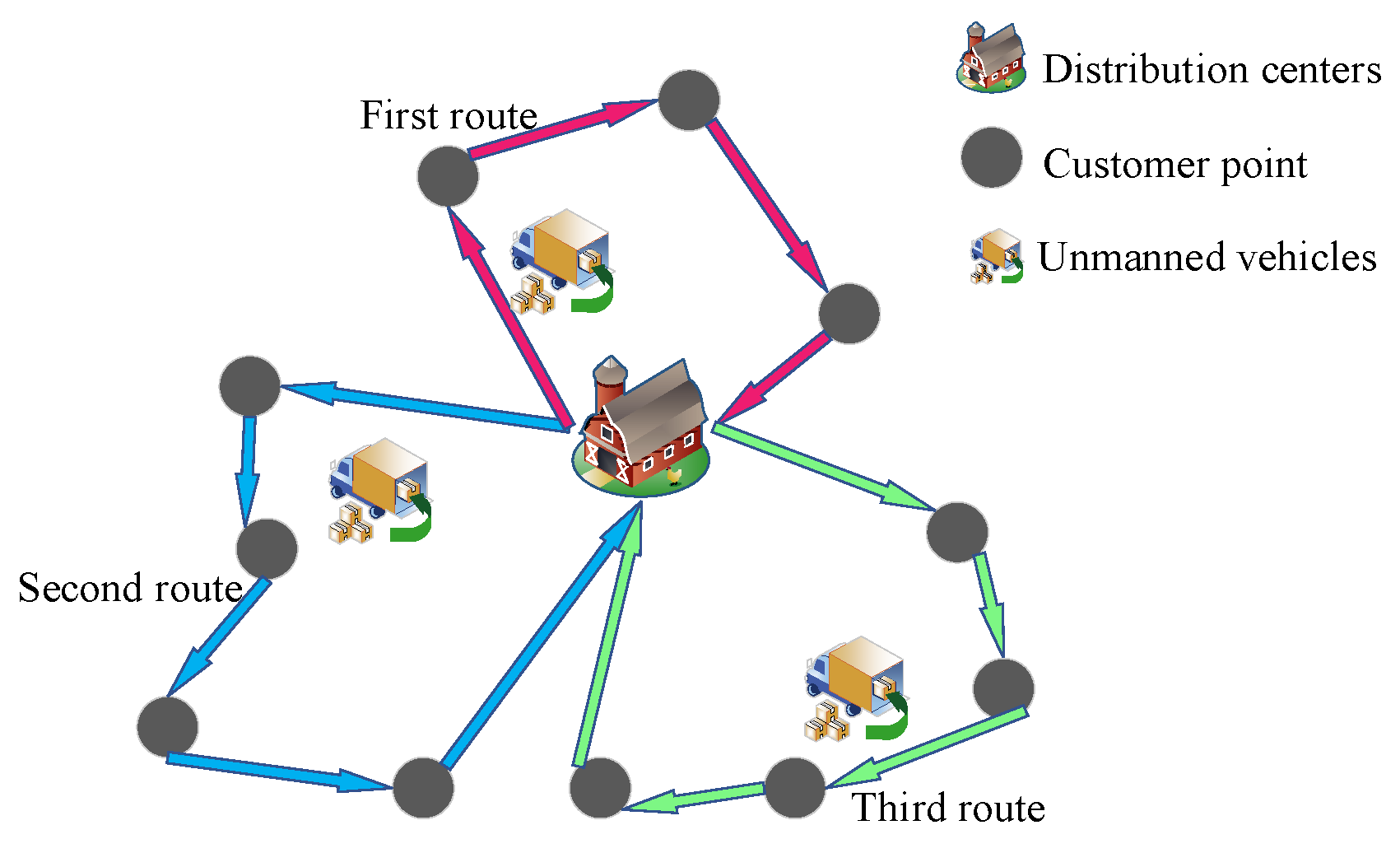
2. Modeling the MTSP for Cooperative Operation of Multiple Unmanned Vehicles
2.1. Problem Description
2.2. Model Building
3. Combinatorial Optimization Algorithm for Solving MTSP
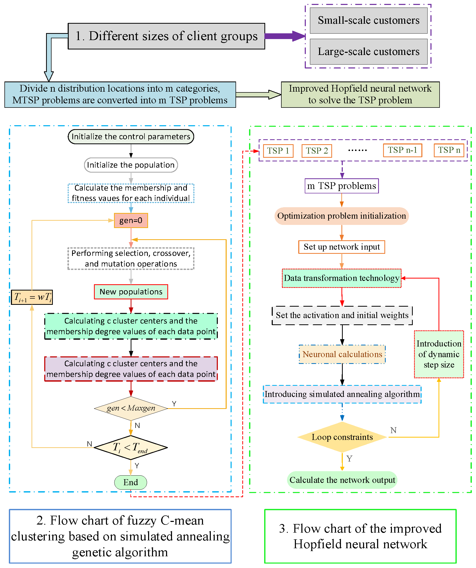
3.1. Fuzzy C-Means Clustering Algorithm (FCM)
3.2. Fuzzy C-Means Algorithm for Genetic Algorithm with Strengthening Using Simulated Annealing (SA-GA-FCM)
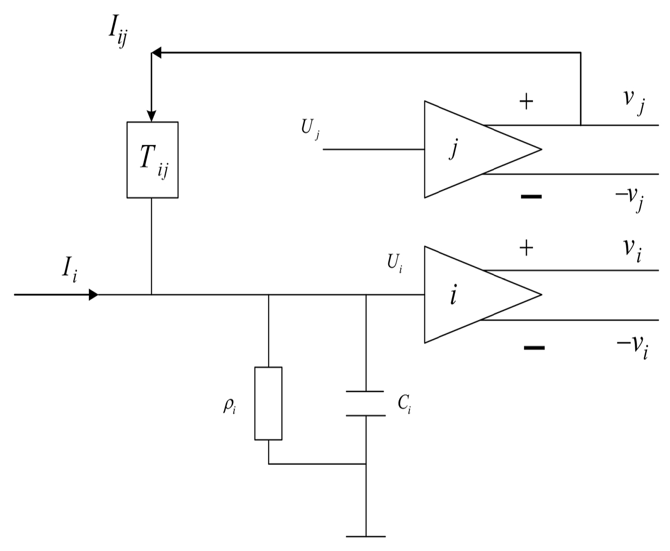
3.3. Hopfield Neural Network
3.4. Improved Hopfield Neural Network (IHNN)
3.4.1. Application of Data Transformation Techniques
3.4.2. Introduction of Dynamic Step Size
3.4.3. Introducing Simulated Annealing Algorithm (SA)
3.4.4. Steps to Improve Hopfield Neural Network to Solve TSP
- (i)
- Set initial values and weights, including , , , and ;
- (ii)
- Read in the distance between clients ();
- (iii)
- Initialization of HNN input , where and is a random value in the interval (−1,1);
- (iv)
- Calculation of using dynamic equations and calculation of in Equation (20) based on the first-order Eulerian method, where after the introduction of the dynamic step is Equation (27);
- (v)
- The sigmoid function is used to calculate in Equation (21);
- (vi)
- Introducing a data transformation technique to smooth the output signal ;
- (vii)
- Calculate the energy function , introducing the simulated annealing algorithm to make the energy more inclined to the direction of gradient descent;
- (viii)
- Check the legitimacy of the path, determine whether the iteration is over, and if not, return to step (iv);
- (ix)
- Output the energy function, the path length, and the energy change.
4. Evaluation and Design Analysis
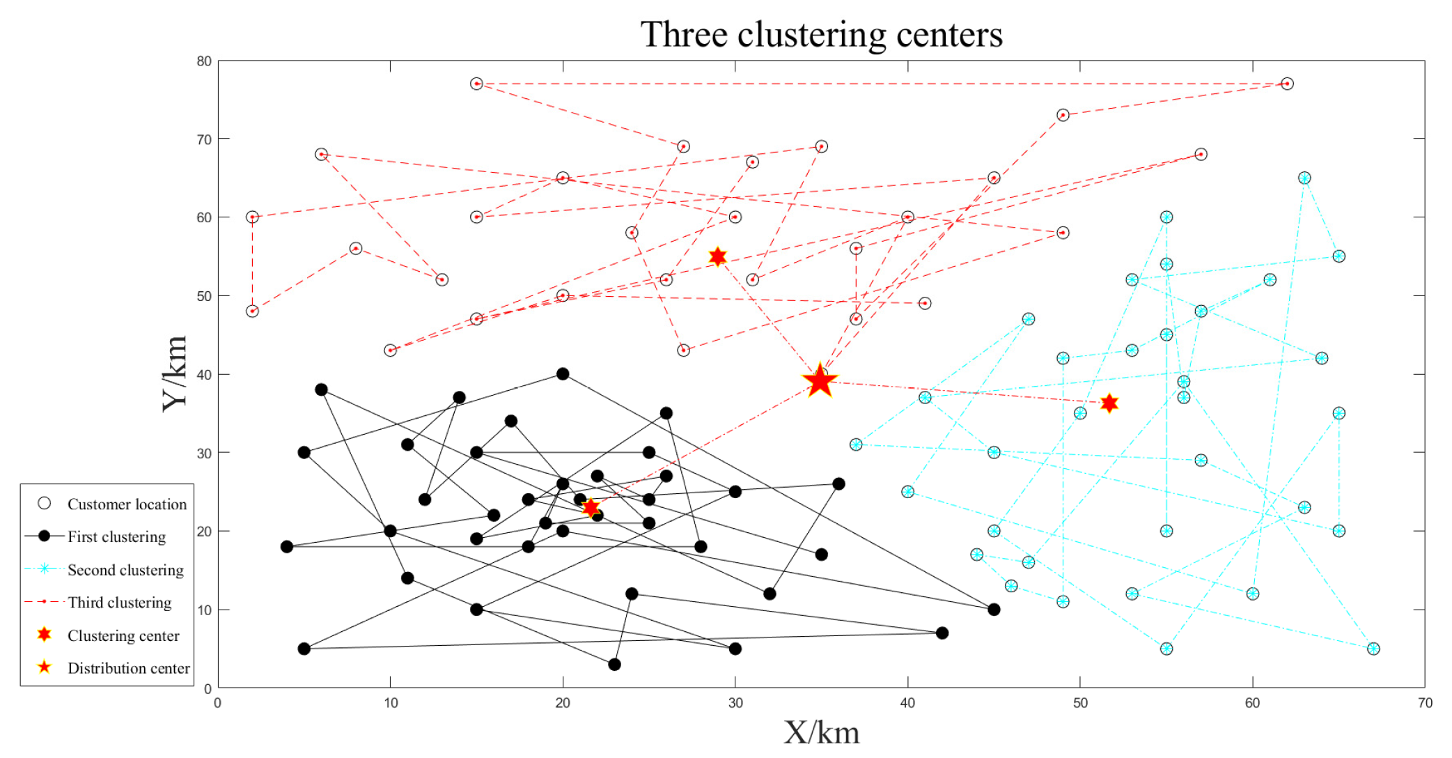
4.1. Simulating Combinatorial Optimization Algorithms (IHNN) on Small-Scale Instances
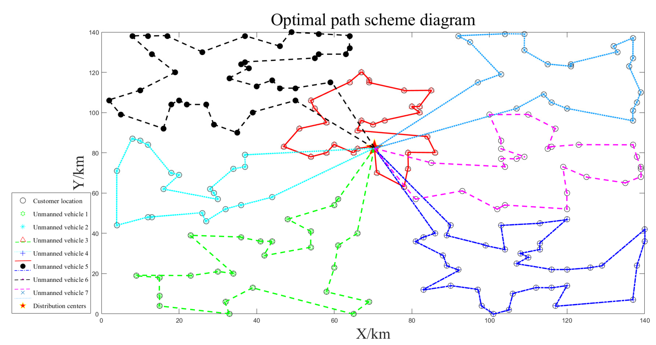
4.2. Combinatorial Optimization Algorithm Large-Scale Simulation Case
5. Comparative Analysis of the IHNN with the Second-Order Oscillation Particle Swarm Optimization (SO-PSO) and the Hybrid Genetic Ant Colony Optimization (GA-ACA)
5.1. Second-Order Oscillation Particle Swarm Optimization (SO-PSO)
5.1.1. Proposal of Particle Swarm Optimization (PSO)
5.1.2. SO-PSO Implementation Steps
- (i)
- Random initialization of particle position and velocity.
- (ii)
- Evaluate particulate individuals, update , and store all optimal individuals in PU.
- (iii)
- If the current number of evolutionary generations is less than 1/2 of the maximum number of generations, update as follows, where , . Similarly, if the current number of evolutionary generations is less than 1/2 of the maximum number of evolutions, then , are taken.
- (iv)
- Compare the adaptive value of the particle itself with the highest value in evolution and, if superior to the highest value, update to its own position.
- (v)
- Make a comparison with the and the gb, and update .
- (vi)
- If the evolution end condition is satisfied, the optimum result is output; otherwise, go to step (iii).
5.2. Hybrid Genetic Ant Colony Algorithm (GA-ACA)
5.2.1. Proposal of GA-ACA
5.2.2. The Concrete Steps for the Implementation of the Hybrid Genetic Ant Colony Algorithm (GA-ACA)
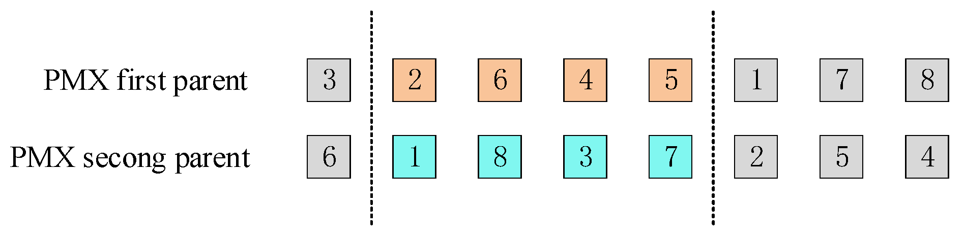
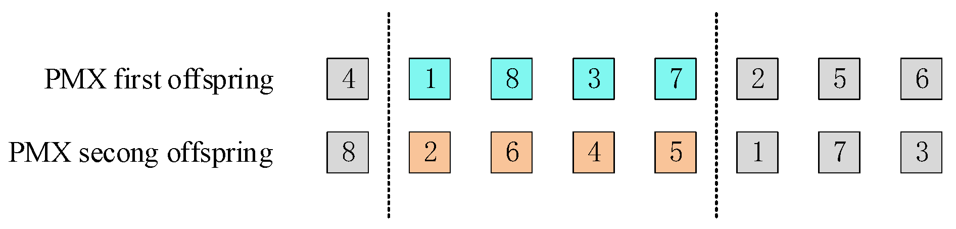
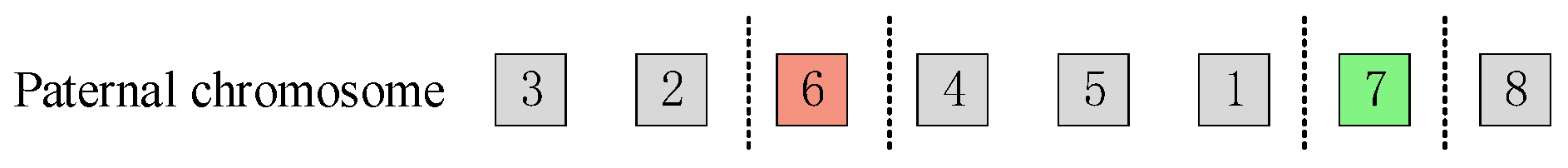
- (i)
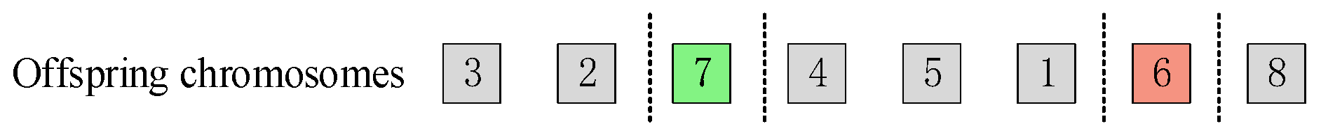
- Encoding. For a TSP containing cities, an array of length represents a solution, e.g., if the cities are numbered , then the encoded bit string of a particular chromosome may be , indicating that the cities are accessed in the order 4-1-8-3-7-4-2-5-6.
- (ii)
- Setup parameters. , the popsize is , and , .
- (iii)
- Calculate the fitness value of the chromosome, opt for roulette operation, and the probability value of the selection of individual is
- (iv)
- (v)
- (vi)
- Start the iteration and determine whether to reach the maximum number of evolutions. If so, go to the next session; otherwise, go to (iii).
- (vii)
- After the evolution is completed, reach an optimized solution as a way to initialize the initial value of the pheromone and related parameters, including , , , , , , and .
- (viii)
- Ants start pathfinding according to the state transfer formula.
- (ix)
- Local pheromones and global pheromones are updated with the path search of ant populations.
- (x)
- Make a judgment that if the current number of evolutions is greater than the limit, the optimal result is output; otherwise, go to step (ix) to continue the iteration.
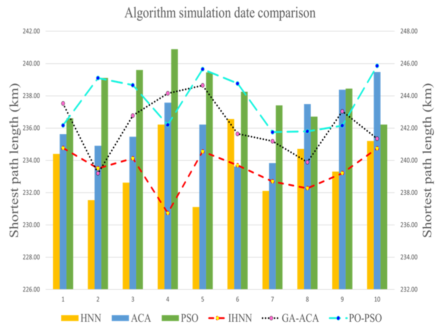
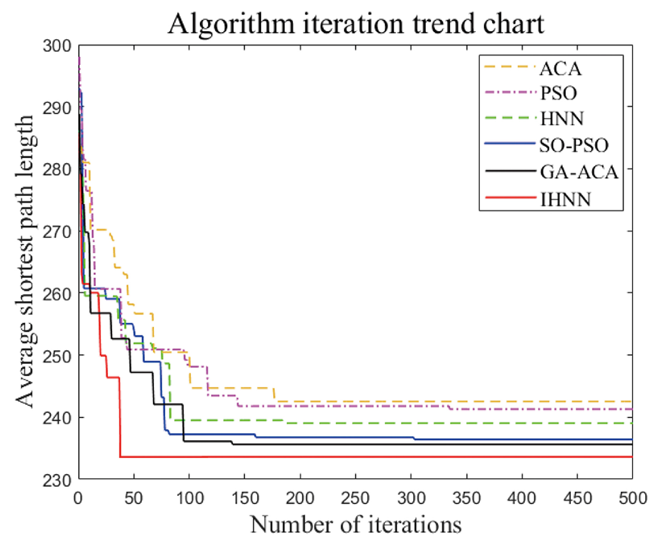
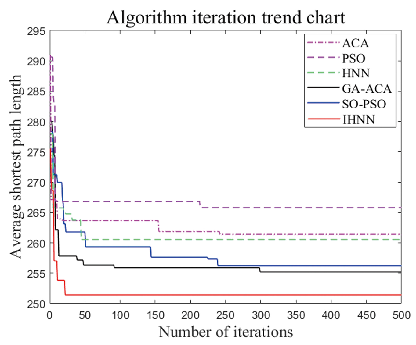
5.3. Comparative Analysis of Three Algorithm Simulations
6. Conclusions
Author Contributions
Funding
Institutional Review Board Statement
Informed Consent Statement
Data Availability Statement
Conflicts of Interest
References
- Severino, A.; Curto, S.; Barberi, S.; Arena, F.; Pau, G. Autonomous Vehicles: An Analysis Both on Their Distinctiveness and the Potential Impact on Urban Transport Systems. Appl. Sci. 2021, 11, 3604. [Google Scholar] [CrossRef]
- Zhang, S.; Markos, C.; James, J.Q. Autonomous vehicle intelligent system: Joint ride-sharing and parcel delivery strategy. IEEE Trans. Intell. Transp. Syst. 2022, 23, 18466–18477. [Google Scholar] [CrossRef]
- Vlachos, I.P.; Pascazzi, R.M.; Zobolas, G.; Repoussis, P.; Giannakis, M. Lean manufacturing systems in the area of Industry 4.0: A lean automation plan of AGVs/IoT integration. Prod. Plan. Control 2023, 34, 345–358. [Google Scholar] [CrossRef]
- Wang, N.; Lyu, Y.; Jia, S.; Zheng, C.; Meng, Z.; Chen, J. A dynamic graph-based many-to-one ride-matching approach for shared autonomous electric vehicles. Transportation 2023, 4, 1–27. [Google Scholar] [CrossRef]
- Stoma, M.; Dudziak, A.; Caban, J.; Droździel, P. The Future of Autonomous Vehicles in the Opinion of Automotive Market Users. Energies 2021, 14, 4777. [Google Scholar] [CrossRef]
- Hakak, S.; Gadekallu, T.R.; Maddikunta, P.K.R.; Ramu, S.P.; Parimala, M.; De Alwis, C.; Liyanage, M. Autonomous Vehicles in 5G and beyond: A Survey. Veh. Commun. 2022, 39, 100551. [Google Scholar] [CrossRef]
- Ahangar, M.N.; Ahmed, Q.Z.; Khan, F.A.; Hafeez, M. A Survey of Autonomous Vehicles: Enabling Communication Technologies and Challenges. Sensors 2021, 21, 706. [Google Scholar] [CrossRef] [PubMed]
- Parekh, D.; Poddar, N.; Rajpurkar, A.; Chahal, M.; Kumar, N.; Joshi, G.P.; Cho, W. A Review on Autonomous Vehicles: Progress, Methods and Challenges. Electronics 2022, 11, 2162. [Google Scholar] [CrossRef]
- Ahmed, H.U.; Huang, Y.; Lu, P.; Bridgelall, R. Technology Developments and Impacts of Connected and Autonomous Vehicles: An Overview. Smart Cities 2022, 5, 382–404. [Google Scholar] [CrossRef]
- Gokasar, I.; Pamucar, D.; Deveci, M.; Ding, W. A novel rough numbers based extended MACBETH method for the prioritization of the connected autonomous vehicles in real-time traffic management. Expert Syst. Appl. 2023, 211, 118445. [Google Scholar] [CrossRef]
- Na, Y.; Li, Y.; Chen, D.; Yao, Y.; Li, T.; Liu, H.; Wang, K. Optimal Energy Consumption Path Planning for Unmanned Aerial Vehicles Based on Improved Particle Swarm Optimization. Sustainability 2023, 15, 12101. [Google Scholar] [CrossRef]
- Van Huynh, D.; Do-Duy, T.; Nguyen, L.D.; Le, M.T.; Vo, N.S.; Duong, T.Q. Real-time optimized path planning and energy consumption for data collection in unmanned ariel vehicles-aided intelligent wireless sensing. IEEE Trans. Ind. Inform. 2021, 18, 2753–2761. [Google Scholar] [CrossRef]
- Yu, X.; Li, C.; Yen, G.G. A knee-guided differential evolution algorithm for unmanned aerial vehicle path planning in disaster management. Appl. Soft Comput. 2021, 98, 106857. [Google Scholar] [CrossRef]
- Chapman, G.H.; Dufort, B. Using laser defect avoidance to build large-area FPGAs. IEEE Des. Test Comput. 1998, 15, 75–81. [Google Scholar] [CrossRef]
- Ding, Y.; Du, X.; Wang, C.; Tian, W.; Deng, C.; Li, K.; Wang, Z. Path Planning for Conformal Antenna Surface Detection Based on Improved Genetic Algorithm. Appl. Sci. 2023, 13, 10490. [Google Scholar] [CrossRef]
- Li, Y.; Zhang, S.; Chen, J.; Jiang, T.; Ye, F. Multi-UAV cooperative mission assignment algorithm based on ACO method. In Proceedings of the 2020 International Conference on Computing, Networking and Communications (ICNC), Big Island, HI, USA, 17–20 February 2020; IEEE: New York, NY, USA, 2020; pp. 304–308. [Google Scholar] [CrossRef]
- Qin, H.; Shao, S.; Wang, T.; Yu, X.; Jiang, Y.; Cao, Z. Review of Autonomous Path Planning Algorithms for Mobile Robots. Drones 2023, 7, 211. [Google Scholar] [CrossRef]
- Gündüz, F.; Birogul, S.; Kose, U. Proof of Optimum (PoO): Consensus Model Based on Fairness and Efficiency in Blockchain. Appl. Sci. 2023, 13, 10149. [Google Scholar] [CrossRef]
- Gao, Z.; Yu, W.; Liu, Z. Exact Algorithms for Some Variants of the Min-Max k-Traveling Salesmen Problem on a Tree. J. East China Univ. Sci. Technol. 2021, 47, 769–778. [Google Scholar] [CrossRef]
- He, P.; Hao, J. Memetic search for the minmax multiple traveling salesman problem with single and multiple depots. Eur. J. Oper. Res. 2023, 307, 1055–1070. [Google Scholar] [CrossRef]
- He, P.; Hao, J. Hybrid search with neighborhood reduction for the multiple traveling salesman problem. Comput. Oper. Res. 2022, 142, 105726. [Google Scholar] [CrossRef]
- Dong, Y.; Wu, Q.; Wen, J. An improved shuffled frog-leaping algorithm for the minmax multiple traveling salesman problem. Neural Comput. Appl. 2021, 33, 17057–17069. Available online: https://link.springer.com/article/10.1007/s00521-021-06298-8/metrics (accessed on 20 September 2023). [CrossRef]
- Kloster, K.; Moeini, M.; Vigo, D.; Wendt, O. The multiple traveling salesman problem in presence of drone-and robot-supported packet stations. Eur. J. Oper. Res. 2023, 305, 630–643. [Google Scholar] [CrossRef]
- Changdar, C.; Mondal, M.; Giri, P.K.; Nandi, U.; Pal, R.K. A two-phase ant colony optimization based approach for single depot multiple travelling salesman problem in Type-2 fuzzy environment. Artif. Intell. Rev. 2023, 56, 965–993. Available online: https://link.springer.com/article/10.1007/s10462-022-10190-9/metrics (accessed on 20 September 2023). [CrossRef]
- Wang, Z.; Fang, X.; Li, H.; Jin, H. An improved partheno-genetic algorithm with reproduction mechanism for the multiple traveling salesperson problem. IEEE Access 2020, 8, 102607–102615. [Google Scholar] [CrossRef]
- Rinaldi, M.; Primatesta, S.; Bugaj, M.; Rostáš, J.; Guglieri, G. Development of Heuristic Approaches for Last-Mile Delivery TSP with a Truck and Multiple Drones. Drones 2023, 7, 407. [Google Scholar] [CrossRef]
- Ivković, N.; Kudelić, R.; Golub, M. Adjustable Pheromone Reinforcement Strategies for Problems with Efficient Heuristic Information. Algorithms 2023, 16, 251. [Google Scholar] [CrossRef]
- Ayari, A.; Sadok, B. PSO-based Dynamic Distributed Algorithm for Automatic Task Clustering in a Robotic Swarm. Pro. Comp. Sci. 2019, 159, 1103–1112. [Google Scholar] [CrossRef]
- Xu, L.K.; Su, S.B.; He, C. Neighborhood Greedy Harris Hawks Optimization for Solving MTSP on the Cubic Surface. Comput. Digit. Eng. 2022, 50, 1869–1875. [Google Scholar]
- Cornejo-Acosta, J.A.; García-Díaz, J.; Pérez-Sansalvador, J.C.; Segura, C. Compact Integer Programs for Depot-Free Multiple Traveling Salesperson Problems. Mathematics 2023, 11, 3014. [Google Scholar] [CrossRef]
- Schuetz, M.J.; Brubaker, J.K.; Katzgraber, H.G. Combinatorial optimization with physics-inspired graph neural networks. Nat. Mach. Intell. 2022, 4, 367–377. [Google Scholar] [CrossRef]
- Hopfield, J.; Tank, D. Neural Computation of Decisions in Optimization Problems. Biol. Cybern 1985, 52, 141–152. [Google Scholar] [CrossRef]
- Lin, Z.; Fan, Z. A Ferroelectric Memristor-Based Transient Chaotic Neural Network for Solving Combinatorial Optimization Problems. Symmetry 2023, 15, 59. [Google Scholar] [CrossRef]
- García, L.; Talaván, P.M.; Yáñez, J. The 2-opt behavior of the Hopfield Network applied to the TSP. Oper. Res. 2022, 22, 1127–1155. [Google Scholar] [CrossRef]
- Zhang, S.; Yu, Y.; Geng, L. Stability analysis of fractional-order Hopfield neural networks with time-varying external inputs. Neural Process. Lett. 2017, 45, 223–241. [Google Scholar] [CrossRef]
- Saadatmand-Tarzjan, M. On Computational Complexity of the Constructive-Optimizer Neural Network for the Traveling Salesman Problem. Neurocomputing 2018, 321, 82–91. [Google Scholar] [CrossRef]
- Hu, Y.; Yao, Y.; Lee, W.S. A reinforcement learning approach for optimizing multiple traveling salesman problems over graphs. Knowledge-Based Syst. 2020, 204, 106244. [Google Scholar] [CrossRef]
- Ling, Z.; Zhou, Y.; Zhang, Y. Solving multiple travelling salesman problem through deep convolutional neural network. IET Cyber-Syst. Robot. 2023, 5, e12084. [Google Scholar] [CrossRef]
- Alves, R.; Silva, C.E.; Souza, J.R. Online Route Scheduling for a Team of Service Robots with MOEAs and mTSP Model. In Proceedings of the International Conference on Engineering Applications of Neural Networks, Crete, Greece, 17–20 June 2022; Springer International Publishing: Cham, Switzerland, 2022; pp. 448–460. [Google Scholar] [CrossRef]
- Ahsini, Y.; Díaz-Masa, P.; Inglés, B.; Rubio, A.; Martínez, A.; Magraner, A.; Conejero, J.A. The Electric Vehicle Traveling Salesman Problem on Digital Elevation Models for Traffic-Aware Urban Logistics. Algorithms 2023, 16, 402. [Google Scholar] [CrossRef]
- Lee, G.M.; Gao, X. A Hybrid Approach Combining Fuzzy c-Means-Based Genetic Algorithm and Machine Learning for Predicting Job Cycle Times for Semiconductor Manufacturing. Appl. Sci. 2021, 11, 7428. [Google Scholar] [CrossRef]
- Abdellahoum, H.; Mokhtari, N.; Brahimi, A.; Boukra, A. CSFCM: An improved fuzzy C-Means image segmentation algorithm using a cooperative approach. Expert Syst. Appl. 2021, 166, 114063. [Google Scholar] [CrossRef]
- Chui, K.T. Driver stress recognition for smart transportation: Applying multiobjective genetic algorithm for improving fuzzy c-means clustering with reduced time and model complexity. Sustain. Comput. Inform. Syst. 2022, 35, 100668. [Google Scholar] [CrossRef]
- Wang, M.; Wang, H.; Feng, Y.; He, Y.; Han, Z.; Zhang, B. Investigating Urban Underground Space Suitability Evaluation Using Fuzzy C-Mean Clustering Algorithm—A Case Study of Huancui District, Weihai City. Appl. Sci. 2022, 12, 12113. [Google Scholar] [CrossRef]
- Zhou, J.; Chen, L.; Li, T. Fuzzy C-mean clustering algorithm based on genetic simulated annealing algorithm battlefield site selection. In Proceedings of the International Conference on Automation Control, Algorithm, and Intelligent Bionics (ACAIB 2023), Xiamen, China, 28–30 April 2023; SPIE: Bellingham, WA, USA, 2023; Volume 12759, pp. 425–434. [Google Scholar] [CrossRef]
- Wang, J.; Xia, J.; Tan, D.; Lin, R.; Su, Y.; Zheng, C.H. scHFC: A hybrid fuzzy clustering method for single-cell RNA-seq data optimized by natural computation. Brief. Bioinform. 2022, 23, bbab588. [Google Scholar] [CrossRef] [PubMed]
- Zhang, X.; Zhou, J.; Chen, W. Data-driven fault diagnosis for PEMFC systems of hybrid tram based on deep learning. Int. J. Hydrog. Energy 2020, 45, 13483–13495. [Google Scholar] [CrossRef]
- Zhang, Y.; Chen, B.; Li, L.; Xu, Y.; Wei, S.; Wang, Y. The Effect of Blue Noise on the Optimization Ability of Hopfield Neural Network. Appl. Sci. 2023, 13, 6028. [Google Scholar] [CrossRef]
- Liu, Y.; Xu, W. Application of improved Hopfield Neural Network in path planning. J. Phys. Conf. Ser. 2020, 1544, 012154. [Google Scholar] [CrossRef]
- Jolai, F.; Ghanbari, A. Integrating data transformation techniques with Hopfield neural networks for solving travelling salesman problem. Expert Syst. Appl. 2010, 37, 5331–5335. [Google Scholar] [CrossRef]
- Urolagin, S.; Sharma, N.; Datta, T.K. A combined architecture of multivariate LSTM with Mahalanobis and Z-Score transformations for oil price forecasting. Energy 2021, 231, 120963. [Google Scholar] [CrossRef]
- Wu, J.; Duan, Q. An algorithm for solving travelling salesman problem based on improved particle swarm optimisation and dynamic step Hopfield network. Int. J. Veh. Des. 2023, 91, 208–231. [Google Scholar] [CrossRef]
- Zhong, C.; Chu, Z.; Luo, C.; Gan, W. A continuous hopfield neural network based on dynamic step for the traveling salesman problem. In Proceedings of the 2017 International Joint Conference on Neural Networks (IJCNN 2017), Anchorage, AK, USA, 14–19 May 2017; IEEE: New York, NY, USA, 2017; pp. 3318–3323. [Google Scholar] [CrossRef]
- Zhou, Y.; Wang, J.; Yin, J. Cooperative annealing Hopfield network for unconstrained binary quadratic programming problem. Expert Syst. Appl 2011, 38, 13894–13905. [Google Scholar] [CrossRef]
- Solomon, M.M. Algorithms for the vehicle routing and scheduling problems with time window constraints. Oper. Res. 1987, 35, 254–265. [Google Scholar] [CrossRef]
- Gehring, H.; Homberger, J. A parallel hybrid evolutionary metaheuristic for the vehicle routing problem with time windows. In Parallel and Distributed Processing, Proceedings of EUROGEN99, San Juan, Puerto Rico, 12–16 April 1999; Springer: Berlin/Heidelberg, Germany, 1999; Volume 2, pp. 57–64. Available online: http://citations.springer.com/item?doi=10.1007/BFb0097899 (accessed on 20 September 2023).
- Wang, F.; Zhang, H.; Zhou, A. A particle swarm optimization algorithm for mixed-variable optimization problems. Swarm Evol. Comput. 2021, 60, 100808. [Google Scholar] [CrossRef]
- Nayyef, H.M.; Ibrahim, A.A.; Mohd Zainuri, M.A.A.; Zulkifley, M.A.; Shareef, H. A Novel Hybrid Algorithm Based on Jellyfish Search and Particle Swarm Optimization. Mathematics 2023, 11, 3210. [Google Scholar] [CrossRef]
- Lin, K.; Zhang, L.; Huang, L.; Feng, Z.; Chen, T. Improved Particle Swarm Path Planning Algorithm with Multi-Factor Coupling in Forest Fire Spread Scenarios. Fire 2023, 6, 202. [Google Scholar] [CrossRef]
- Deng, L.; Chen, H.; Zhang, X.; Liu, H. Three-Dimensional Path Planning of UAV Based on Improved Particle Swarm Optimization. Mathematics 2023, 11, 1987. [Google Scholar] [CrossRef]
- Tezel, B.T.; Mert, A. A cooperative system for metaheuristic algorithms. Expert Syst. Appl. 2021, 165, 113976. [Google Scholar] [CrossRef]
- Xia, X.; Gong, M.; Wang, T.; Liu, Y.; Zhang, H.; Zhang, Z. Parameter Identification of the Yoshida-Uemori Hardening Model for Remanufacturing. Metals 2021, 11, 1859. [Google Scholar] [CrossRef]
- Martínez-Vargas, A.; Gómez-Avilés, J.A.; Cosío-León, M.A.; Andrade, Á.G. Explaining the Walking Through of a Team of Algorithms. Computer 2023, 56, 67–81. [Google Scholar] [CrossRef]
- Etminaniesfahani, A.; Gu, H.; Salehipour, A. ABFIA: A hybrid algorithm based on artificial bee colony and Fibonacci indicator algorithm. J. Comput. Sci. 2022, 61, 101651. [Google Scholar] [CrossRef]
- Di Caprio, D.; Ebrahimnejad, A.; Alrezaamiri, H.; Santos-Arteaga, F.J. A novel ant colony algorithm for solving shortest path problems with fuzzy arc weights. Alex. Eng. J. 2022, 61, 3403–3415. [Google Scholar] [CrossRef]
- Gunay-Sezer, N.S.; Cakmak, E.; Bulkan, S. A Hybrid Metaheuristic Solution Method to Traveling Salesman Problem with Drone. Systems 2023, 11, 259. [Google Scholar] [CrossRef]
- Ma, X.; Bian, W.; Wei, W.; Wei, F. Customer-Centric, Two-Product Split Delivery Vehicle Routing Problem under Consideration of Weighted Customer Waiting Time in Power Industry. Energies 2022, 15, 3546. [Google Scholar] [CrossRef]
- Sun, Z.; Gu, X. Hybrid Algorithm Based on an Estimation of Distribution Algorithm and Cuckoo Search for the No Idle Permutation Flow Shop Scheduling Problem with the Total Tardiness Criterion Minimization. Sustainability 2017, 9, 953. [Google Scholar] [CrossRef]


| Article | Optimization Models | Solution Method | ||||||
|---|---|---|---|---|---|---|---|---|
| Problem | Research Background | Objective Function | Research Object | Specific Constraints | Heuristics Algorithms | Precision Algorithms | Others | |
| TSP | Ding et al. [15] (2023) | Conformal antenna surface detection | Minimum path length | The conformal antenna | General constraints and elimination of subloop constraints | Hybrid genetic algorithm | ||
| Gündüz et al. [18] (2023) | blockchain technology | The block generation time | System node | General constraints and elimination of subloop constraints | Consensus algorithm | |||
| Lin et al. [33] (2023) | Hardware implementation based on memristors | Obtaining the shortest path | Ferroelectric memristor | General constraints and elimination of subloop constraints | Ferroelectric memristor-based transient chaotic neural network (FM-TCNN) | |||
| García et al. [34] (2022) | The attraction basins of the CHN | Obtaining the shortest path | Traveling salesman | General constraints and elimination of subloop constraints | Continuous Hopfield network (CHN) | |||
| Ahsini et al. [40] (2023) | Logistics distribution | Minimization of travel costs | Electric delivery trucks | Distance and elevation, as in Graser | Artificial neural network (ANN) | |||
| MTSP | Gao et al. [19] (2021) | MTSP in tree structure | Min–Max k-TSPT | Travel agent | Min–Max k-Traveling Salesmen Problem on a Tree | Pseudo-polynomial exact algorithms | ||
| He and Hao [20] (2023) | Minimize the longest stroke in the trip | Traveling salesman | Multiple depots and closed path | A unified population-based memetic algorithm (MA) | ||||
| He and Hao [21] (2022) | Minimize the total traveling distance | Traveling salesman | Multiple depots and closed path | Hybrid algorithm with neighborhood reduction | ||||
| Dong et al. [22] (2021) | Minimizing the total distance traveled | Traveling salesman | Multiple depots and closed path | Improved shuffled frog-leaping algorithm (ISFLA) | ||||
| Kloster et al. [23] (2023) | The multiple Traveling Salesman Problem with Drone Stations (mTSP-DS) | Minimizing service time | Drone stations | Number of self-driving cars | Metaheuristic approach | |||
| Wang et al. [25] (2020) | Minimum cost circuit | Traveling salesman | Multiple depots and closed path | Partheno-Genetic algorithm with reproduction mechanism (RIPGA) | ||||
| Rinaldi et al. [26] (2023) | logistics distribution | Minimize the total completion time | A truck and multiple drones | Multiple time window constraints | Hybrid genetic algorithm | |||
| Ivković et al. [27] (2023) | Minimizing the total distance traveled | Traveling salesman | Multiple depots and closed path | Ant colony optimization (ACO) | ||||
| Aaa et al. [28] (2019) | The Multi-Robot Task Allocation (MRTA) | Minimizing the total distance traveled | Multi-Robot | Multiple depots and closed path | PSO-based dynamic distributed algorithm | |||
| Cornejo-Acosta et al. [30] (2023) | Minimizing total path cost | Traveling salesman | Multiple boundary constraints | Compact integer programs | ||||
| Hu et al. [37] (2020) | Minimizing the total distance traveled | Traveling salesman | Assignment constraints and elimination of subloop constraints | Graph neural network | ||||
| Difference and similarity | In comparing the aforementioned literature, it is evident that both TSP and MTSP are instances of combinatorial optimization problems, primarily concerned with discovering optimal paths or tour routes. Their similarities and distinctions can be summarized as follows: Firstly, TSP is geared towards determining the shortest path for a single salesperson to visit all designated cities once and return to the initial city. In TSP, the presence of only one salesperson is assumed, and the primary objective is to minimize the cumulative distance traveled or the associated cost. Secondly, MTSP introduces the complexity of multiple salespersons, each tasked with visiting a subset of cities without the requirement to cover all of them. The optimization goals can encompass minimizing the overall distance traveled, cost reduction, or compliance with specific constraints. Thirdly, with regards to solution methodologies, it is noteworthy that, given the NP-hard nature of TSP and MTSP, many researchers have achieved noteworthy outcomes employing heuristic algorithms and neural networks, with fewer instances of exact algorithms being applied. | |||||||
| Indices | |
|---|---|
| Index of the customers’ nodes, | |
| Index of the distribution center | |
| Parameters | |
| Distance from customer to customer | |
| Customer demand at the corresponding node | |
| Total number of customers traveled by unmanned vehicle from the distribution center to customer | |
| Serial number of the unmanned vehicle, | |
| Distance traveled by the th unmanned vehicle | |
| Time after the last customer is worked on by the unmanned vehicle | |
| Maximum load capacity of unmanned vehicle | |
| Unmanned vehicle travel speed | |
| Travelling time of the th unmanned vehicle | |
| Decision Variables | |
| Equal to 1 if the th unmanned vehicle passes through nodes and ; otherwise, 0 | |
| Equal to 1 if the unmanned vehicle passes through arc segment ; otherwise, 0 |
| Reference Distribution Center | Distribution Center (km) | Clustering Situation | Unmanned Vehicles | Clustering Center (km) | Minimum Jr Value | Number of Customers | Path Length (km) | Paths Total Length (km) | Distribution Time (h) | Total Distribution Time (h) |
|---|---|---|---|---|---|---|---|---|---|---|
| (35,35) | (34.92,39.06) | 1 | 1 | (51.69,36.25) | 6.75 × 10³ | 33 | 216.23 | 699.86 | 3.60 | 11.66 |
| 2 | (28.98,54.93) | 29 | 249.99 | 4.17 | ||||||
| 3 | (21.63,22.94) | 38 | 233.64 | 3.89 | ||||||
| (34.51,35.84) | 2 | 1 | (52.69,50.78) | 3.48 × 10³ | 25 | 181.98 | 533.46 | 3.03 | 11.93 | |
| 2 | (46.49,16.97) | 22 | 159.55 | 2.66 | ||||||
| 3 | (22.55,54.70) | 22 | 191.93 | 3.20 | ||||||
| 4 | (19.51,23.50) | 31 | 182.44 | 3.04 | ||||||
| (34.45,39.77) | 3 | 1 | (15.87,45.00) | 2 × 10³ | 17 | 160.96 | 751.18 | 2.68 | 12.52 | |
| 2 | (19.67,22.42) | 29 | 168.19 | 2.80 | ||||||
| 3 | (37.16,57.62) | 15 | 139.41 | 2.32 | ||||||
| 4 | (53.93,45.05) | 18 | 132.23 | 2.21 | ||||||
| 5 | (46.65,15.45) | 21 | 150.39 | 2.51 |
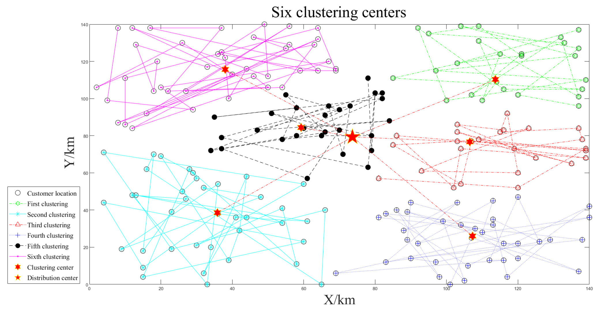
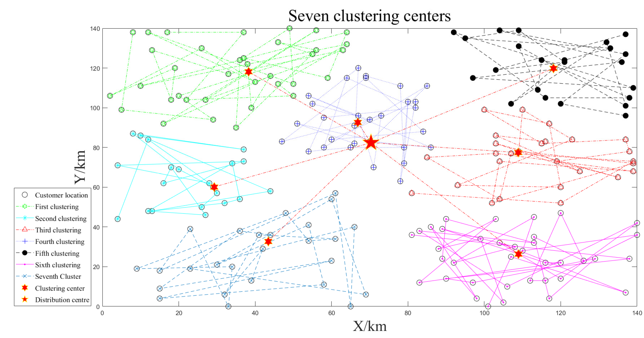
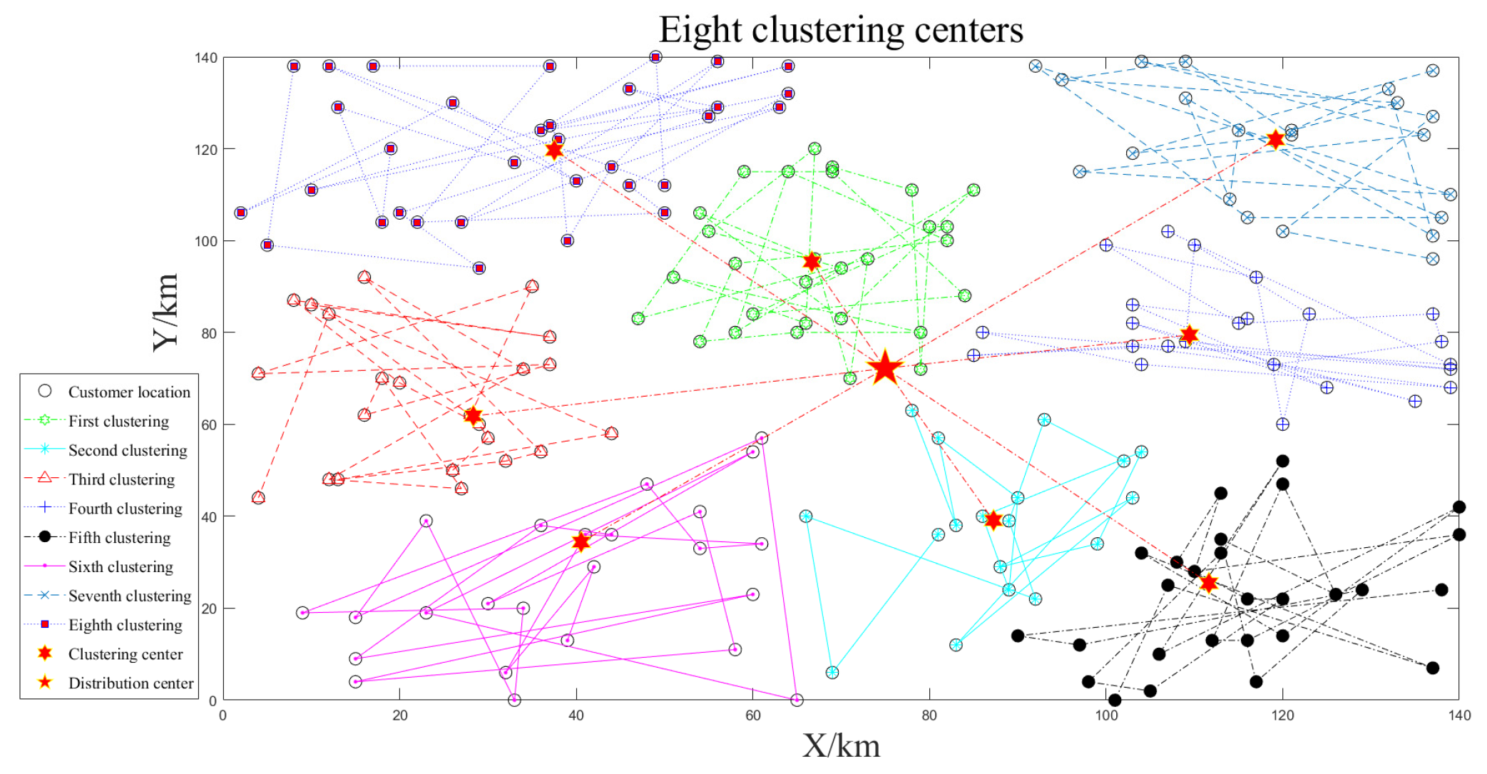
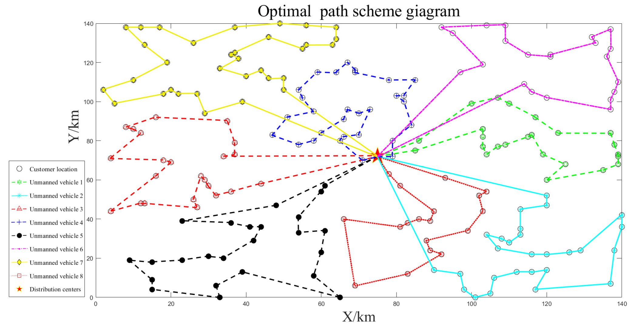
| Reference Distribution Center | Distribution Center (km) | Clustering Situation | Unmanned Vehicles | Clustering Center (km) | Minimum Jr Value | Number of Customers | Path Length (km) | Paths Total Length (km) | Distribution Time (h) | Total Distribution Time (h) |
|---|---|---|---|---|---|---|---|---|---|---|
| (70,70) | (73.61,79.34) | 4 | 1 | (107.27,26.02) | 1.39 × 10⁴ | 28 | 243.73 | 1919.27 | 3.25 | 25.59 |
| 2 | (113.67,110.28) | 27 | 277.50 | 3.70 | ||||||
| 3 | (59.26,84.47) | 38 | 389.70 | 5.20 | ||||||
| 4 | (106.50,76.67) | 25 | 214.10 | 2.85 | ||||||
| 5 | (35.83,38.55) | 39 | 425.41 | 5.67 | ||||||
| 6 | (37.98,115.66) | 43 | 368.83 | 4.92 | ||||||
| (70.36,82.37) | 5 | 1 | (38.23,118.21) | 9.97 × 10³ | 30 | 210.99 | 1993.11 | 2.81 | 26.57 | |
| 2 | (66.86,92.61) | 36 | 339.73 | 4.53 | ||||||
| 3 | (43.44,32.66) | 37 | 371.82 | 4.96 | ||||||
| 4 | (108.94,26.31) | 21 | 233.05 | 3.11 | ||||||
| 5 | (118.12,119.78) | 27 | 255.30 | 3.40 | ||||||
| 6 | (29.29,60.08) | 26 | 325.77 | 4.34 | ||||||
| 7 | (108.86,77.43) | 23 | 256.45 | 3.42 | ||||||
| (74.96,72.22) | 6 | 1 | (40.54,34.36) | 7.54 × 10³ | 24 | 299.06 | 2061.94 | 3.99 | 27.49 | |
| 2 | (109.47,79.43) | 24 | 208.04 | 2.77 | ||||||
| 3 | (111.66,25.39) | 27 | 312.09 | 4.16 | ||||||
| 4 | (87.24,39.10) | 18 | 201.10 | 2.68 | ||||||
| 5 | (118.96,121.88) | 22 | 264.62 | 3.53 | ||||||
| 6 | (66.63,95.35) | 29 | 195.43 | 2.61 | ||||||
| 7 | (37.47,119.81) | 33 | 326.82 | 4.36 | ||||||
| 8 | (28.34,61.83) | 23 | 254.78 | 3.40 |
Disclaimer/Publisher’s Note: The statements, opinions and data contained in all publications are solely those of the individual author(s) and contributor(s) and not of MDPI and/or the editor(s). MDPI and/or the editor(s) disclaim responsibility for any injury to people or property resulting from any ideas, methods, instructions or products referred to in the content. |
© 2023 by the authors. Licensee MDPI, Basel, Switzerland. This article is an open access article distributed under the terms and conditions of the Creative Commons Attribution (CC BY) license (https://creativecommons.org/licenses/by/4.0/).
Share and Cite
Liu, S.; Gao, X.; Chen, L.; Zhou, S.; Peng, Y.; Yu, D.Z.; Ma, X.; Wang, Y. Multi-Traveler Salesman Problem for Unmanned Vehicles: Optimization through Improved Hopfield Neural Network. Sustainability 2023, 15, 15118. https://doi.org/10.3390/su152015118
Liu S, Gao X, Chen L, Zhou S, Peng Y, Yu DZ, Ma X, Wang Y. Multi-Traveler Salesman Problem for Unmanned Vehicles: Optimization through Improved Hopfield Neural Network. Sustainability. 2023; 15(20):15118. https://doi.org/10.3390/su152015118
Chicago/Turabian StyleLiu, Song, Xinhua Gao, Liu Chen, Sihui Zhou, Yong Peng, Dennis Z. Yu, Xianting Ma, and Yan Wang. 2023. "Multi-Traveler Salesman Problem for Unmanned Vehicles: Optimization through Improved Hopfield Neural Network" Sustainability 15, no. 20: 15118. https://doi.org/10.3390/su152015118
APA StyleLiu, S., Gao, X., Chen, L., Zhou, S., Peng, Y., Yu, D. Z., Ma, X., & Wang, Y. (2023). Multi-Traveler Salesman Problem for Unmanned Vehicles: Optimization through Improved Hopfield Neural Network. Sustainability, 15(20), 15118. https://doi.org/10.3390/su152015118