Long-Term Solar Power Time-Series Data Generation Method Based on Generative Adversarial Networks and Sunrise–Sunset Time Correction

Abstract

Constructing long-term solar power time-series data is a challenging task for power system planners. This paper proposes a novel approach to generate long-term solar power time-series data through leveraging Time-series Generative Adversarial Networks (TimeGANs) in conjunction with adjustments based on sunrise–sunset times. A TimeGAN model including three key components, an autoencoder network, an adversarial network, and a supervised network, is proposed for data generation. In order to effectively capture autocorrelation and enhance the fidelity of the generated data, a Recurrent Neural Network (RNN) is proposed to construct each component of TimeGAN. The sunrise and sunset time calculated based on astronomical theory is proposed for adjusting the start and end time of solar power time-series, which are generated by the TimeGAN model. This case study, using real datasets of solar power stations at two different geographic locations, indicates that the proposed method is superior to previous methods in terms of four aspects: annual power generation, probability distribution, fluctuation, and periodicity features. A comparison of production cost simulation results between using the solar power data generated via the proposed method and using the actual data affirms the feasibility of the proposed method.

1. Introduction

Production cost simulation is an important tool for power system planning and operation [1]. Its applications encompass an in-depth analysis of power and energy balance within the power system, facilitating medium and long-term economic planning for the grid, and assessing the integration of renewable energy sources [2,3]. In traditional power systems, production cost simulation primarily revolves around the dynamic generation of power to match fluctuating loads. However, with the introduction of the “carbon peaking and carbon neutrality” goal, the permeability of renewable energy is increasing. In addition to load, the uncertainty of renewable energy sources is increasingly affecting the power system [4]. Moreover, the fluctuation characteristics of renewable energy are more difficult to accurately describe and capture than the load. As a result, existing typical-day and typical-week production cost simulation techniques face challenges when applied in this context [5]. Annual production cost simulation is an effective approach to deal with the uncertainty in new power systems. However, it needs to be based on solar power data for several years or even decades [6,7]. For many newly built solar power stations, the length of existing solar power time-series obviously cannot meet the requirements of production cost simulation [8]. Therefore, it is necessary to propose an effective method for generating solar power time-series data. The length of generated data should meet the requirements of production cost simulation. Furthermore, the generated data should exhibit a high degree of statistical consistency with the historical data, ensuring their suitability for rigorous academic analysis and simulation [9].

Long-term time-series modeling is primarily concerned with replicating the statistical properties of historical data rather than achieving precise data point accuracy [10]. Within this domain, two distinct modeling approaches for generating long-term solar power time-series data are prevalent: indirect modeling and direct modeling. Indirect modeling firstly predicts solar irradiance and then calculates the power according to the solar power generation system model [11,12]. However, it is difficult to comprehensively and accurately obtain astronomical meteorological data when establishing a meteorological model of irradiance. Moreover, solar power is also influenced by meteorological factors such as temperature, relative humidity, wind speed, wind direction, atmospheric pressure, as well as equipment aging [13,14,15]. It is difficult to characterize these complex relationships using indirect modeling methods. Therefore, the adaptability of indirect modeling methods is limited. Direct modeling is to directly generate solar power using the historical data. Compared with indirect modeling methods, direct modeling can capture the variation in solar power more accurately. Meanwhile, it can improve the quality of the generated data and allow for personalized modeling based on different characteristics of the solar power stations. Therefore, direct modeling can better adapt to different power generation environments. Currently, commonly used direct modeling methods include Neural Networks [16,17,18,19], Autoregressive Moving Average Model (ARMA) [20,21], Support Vector Regression (SVR) [22,23,24], and Markov Chains (MCs) [25,26,27]. The ARMA method can effectively capture the autocorrelation of time-series. However, when using a sampling method to generate random sequences, the mean and covariance matrix remain unchanged at different time points. As a result, the ARMA method cannot accurately characterize the probability distribution of time-varying variables over long time scales [28,29]. The SVM model is a non-parametric model that can adapt to various data distributions. However, its ability to capture the trend and seasonality in time-series is relatively weak. Markov Chains have shown good performance in modeling wind farms [30], and they have also been applied in predicting solar power and generating time-series of solar irradiance. In [31], a method based on Markov Chains was proposed to generate global irradiance time-series with one-minute resolution. In [32], a method based on K-means clustering and Markov Chain Monte Carlo was proposed for aggregating solar power data. In [33], a method based on novel scenario partitioning and considering temporal correlation was proposed for simulating solar power time-series. However, Markov Chains can only deal with discrete-state sequences, while solar power data are continuous. Using Markov Chains for continuous solar power data requires discretization. It may lead to information loss. Therefore, it may cause the generated data to differ significantly from the historical data.

The abovementioned solar power modeling methods have some shortcomings in describing the statistical characteristics of solar power and long-term time-series generation. In recent years, Generative Adversarial Networks (GANs) have made some progress in generating long-term time-series [34,35,36]. However, the standard GAN model overlooks internal autocorrelation in time-series data generation. An ideal data generation model should not only learn feature distributions at each time point but also capture complex relationships between variables at different time points. Using the Autoregressive Model (AR) to capture the autocorrelation of time-series has a good effect on addressing the prediction problem [37,38,39]. However, the AR model is naturally deterministic, requiring meaningful and real data as input. Additionally, the AR model does not possess generative capabilities. To address these limitations, Yoon et al. [40] proposed the TimeGAN model via combining the methodologies of the GAN and AR model. The TimeGAN model considers autocorrelation when generating data. This integration improves the quality of the generated data [41,42,43]. In [41,42], the TimeGAN model was used to expand wind power and load data to increase the amount of model training data and improve prediction accuracy. In [43], the expansion of historical solar power data was realized based on TimeGAN. However, the TimeGAN model lacks a supervised network, which makes the generated data quite different from the historical data. Moreover, in order to solve the problem that the solar power time-series generated using TimeGAN is close to but not equal to zero at night, it only takes the historical solar power data with the same time scale and non-zero as input, but this cannot accurately reflect the regular characteristics of solar power data.

Inspired by the TimeGAN model, this paper proposes a long-term solar power time-series data generation method based on TimeGAN and sunrise–sunset time correction. The contributions of this work are as follows: (1) A solar power generation model based on TimeGAN is developed, which includes three key components, an autoencoder network, an adversarial network, and a supervisory network. It takes advantage of the game and mutual learning between generator and discriminator in GAN to solve the problem of long-term time-series generation. (2) An RNN is proposed to build the TimeGAN model to mine the features of data with time-series characteristics. It ensures that the model is autoregressive. (3) The sunrise and sunset time is proposed to approximately replace the start and end time of solar power to correct the generated data, which overcomes the limitation of inaccurate capture of the TimeGAN when dealing with complex time series.

The remaining paper is organized as follows: The relevant knowledge regarding construction and training process of the solar power data generation model based on TimeGAN is introduced in Section 2. In Section 3, a comparison is made between the proposed method and other methods. Section 4 discusses the results obtained from Section 3. The conclusions are provided in the last section.

2. Long-Term Solar Power Time-Series Data Generation Model

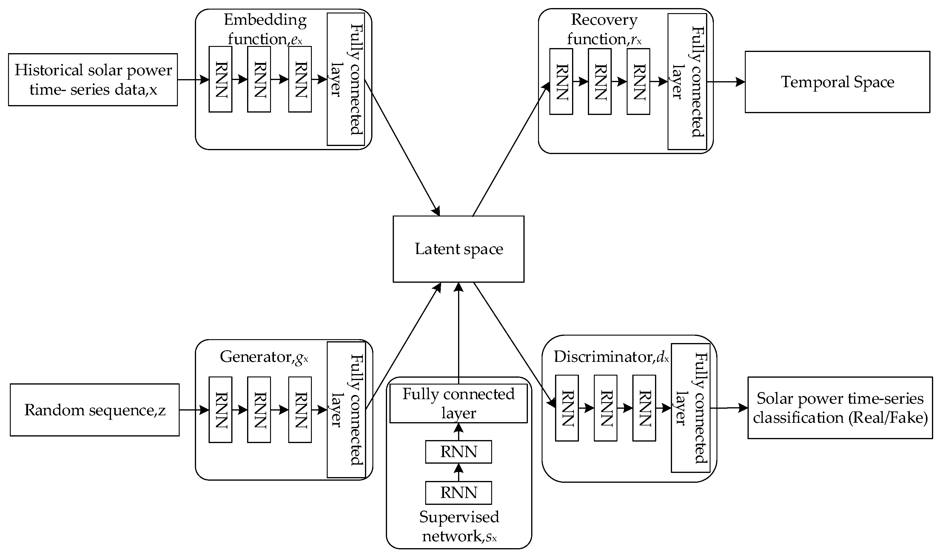
2.1. Solar Power Data Generation Model Based on TimeGAN

In the process of solar power generation, many factors, such as weather type and season, will affect its output. These factors are usually nonlinear and dynamic, so it is difficult to establish a clear and accurate mathematical model. Therefore, it is a challenging task to determine the distribution and characteristics of solar power data. The TimeGAN model can capture the complex structure and characteristics of time-series through learning the key statistical features extracted from historical data. Specifically, the TimeGAN model can generate new time-series through capturing the distribution of a set of random noise vectors and the correlation in the time-series. Accordingly, it is a powerful tool for generating a time-series that conforms to the statistical characteristics of the solar power time-series.

2.1.1. Model Structure

The structure of the solar power data generation model based on TimeGAN is shown in Figure 1. It includes three components: an autoencoder network, an adversarial network, and a supervised network. The autoencoder network is composed of embedding and recovery functions. The adversarial network consists of a generator and a discriminator. The role of the embedding function is to transform the historical data into a vector representation in the latent space. This vector representation can better capture the patterns and structures within the time-series, thereby improving the performance of the generative model. The purpose of the recovery function is to convert the vector representation in the latent space back to temporal space data. The generator takes random data as input, and the generated data are output to the latent space. The discriminator takes the encoded data from the latent space as input, and the output is the result of judging whether the input is true or false. The function of the supervised network is to generate a supervised space for supervised learning.

For time-series, there is a strong correlation between the input data from different time steps. However, the output of traditional neural networks, such as fully connected neural networks or convolutional neural networks, is completely independent of the input and has little correlation with each other. Additionally, these networks lack temporal characteristics, so it is impossible to deeply explore the features of time-series. The RNN introduces the concept of memory. RNN neurons have an additional feedback input. It can save part of the information output by the previous network and pass it to the next layer to participate in the calculation. This enables the establishment of connections between RNN modules at different time steps. Therefore, all networks of the TimeGAN model in this paper are constructed with multiple layers of RNN units. It ensures that the model is autoregressive.

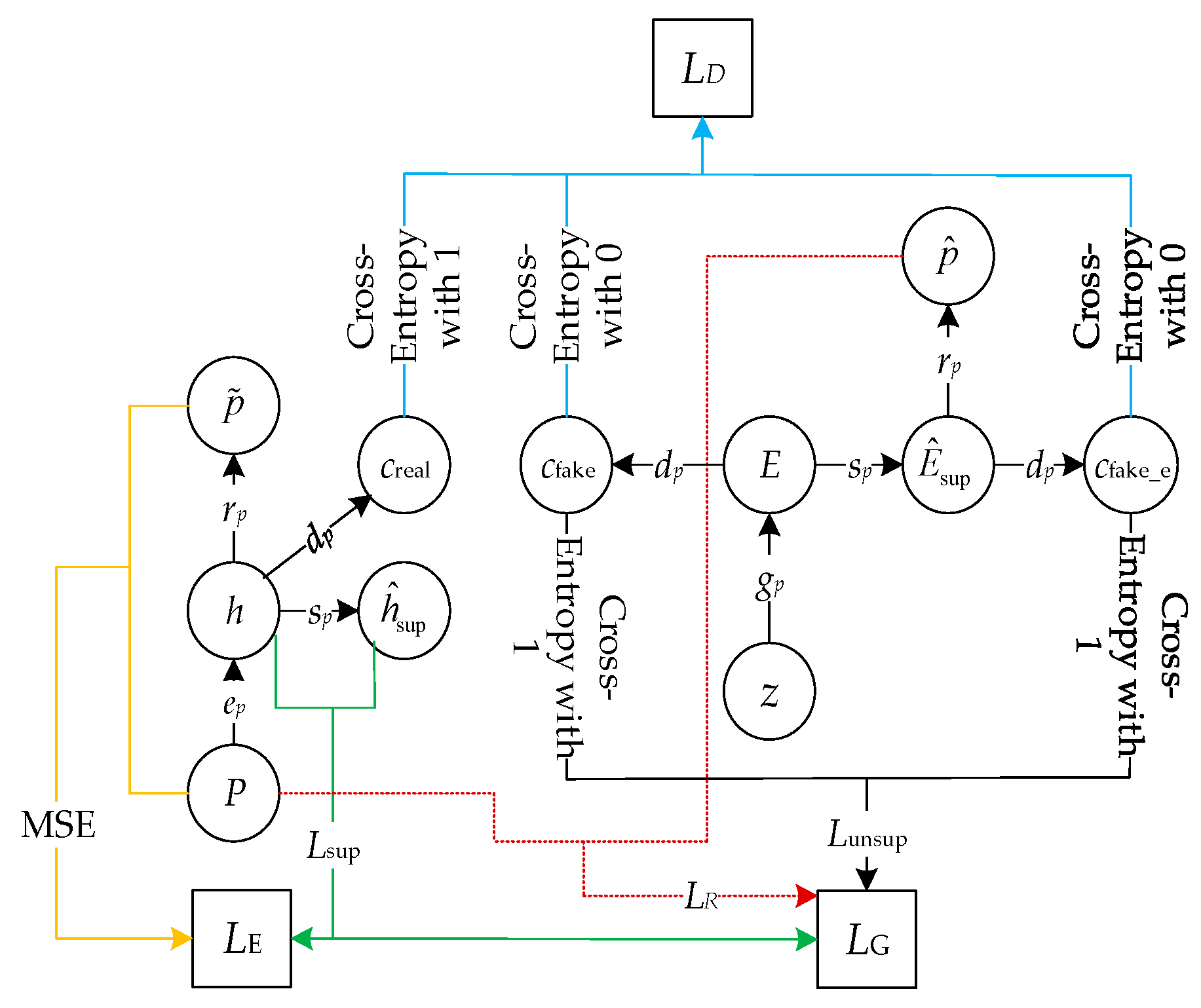
2.1.2. Model Construction

(1) Autoencoder Network Construction

The embedding and recovery functions provide a reversible mapping from the feature space to the latent space. It enables the adversarial network to learn the correlations of the time-series. The embedding function is defined as follows [40]:

$${{\displaystyle h}}_t={{\displaystyle e}}_p({{\displaystyle h}}_{t-1},{{\displaystyle p}}_t)$$

(1)

where ${{\displaystyle e}}_p$ represents the embedding function. It consists of three layers of RNN units and one fully connected layer. The hidden layer has 24 neurons with a sigmoid activation function. ${{\displaystyle p}}_t$ represents the code in the latent space corresponding to the historical solar power data ${{\displaystyle p}}_t$. The subscript t represents the time information. The recovery function is defined as follows [40]:

$${{\displaystyle \tilde{p}}}_t={{\displaystyle r}}_p({{\displaystyle h}}_t)$$

(2)

$${{\displaystyle \widehat{p}}}_t={{\displaystyle r}}_p({{\displaystyle \widehat{E}}}_{\sup ,t})$$

(3)

where ${{\displaystyle r}}_p$ represents the recovery function. It has the same structure as the embedding function. It restores ${{\displaystyle h}}_t$ to data ${{\displaystyle \tilde{p}}}_t$ with the same dimension as the historical solar power data. It also restores the supervised space ${{\displaystyle \widehat{E}}}_{\sup ,t}$ of the generated data to data ${{\displaystyle \widehat{p}}}_t$ with the same dimension as the historical solar power data.

(2) Supervised Network Construction

The expression of historical solar power data corresponding to the latent space encoding ${{\displaystyle h}}_t$ and the generated data ${{\displaystyle E}}_t$ from the generator in the supervised space is given by Equations (4) and (5), respectively [44].

$${{\displaystyle \widehat{h}}}_{\sup ,t}={{\displaystyle s}}_p({{\displaystyle h}}_t)$$

(4)

$${{\displaystyle \widehat{E}}}_{\sup ,t}={{\displaystyle s}}_p({{\displaystyle E}}_t)$$

(5)

where ${{\displaystyle s}}_p$ represents the supervisory function. It consists of two layers of RNN units and one fully connected layer. The activation function is sigmoid. ${{\displaystyle \widehat{h}}}_{\sup ,t}$ and ${{\displaystyle \widehat{E}}}_{\sup ,t}$ represent the expressions of ${{\displaystyle h}}_t$ and ${{\displaystyle E}}_t$ in the supervised space.

(3) Adversarial Network Construction

The data generated by the generator from a random time-series are first generated in the latent space. The corresponding formula for the generator network is as follows [40]:

$${{\displaystyle E}}_t={{\displaystyle g}}_p({{\displaystyle E}}_{t-1},{{\displaystyle z}}_t)$$

(6)

where ${{\displaystyle g}}_p$ represents the generator function. It consists of three layers of RNN units and one fully connected layer. The hidden layer has 24 neurons with a sigmoid activation function. ${{\displaystyle E}}_t$ represents the generated solar power data at time t by the generator. ${{\displaystyle E}}_{t-1}$ represents the previously generated solar power data at the previous time step. ${{\displaystyle z}}_t$ denotes a random time-series of the same dimension as the historical solar power data. It can be from any random process. The discriminator also operates in the latent space, distinguishing among the latent space ${{\displaystyle h}}_t$ of the historical data, the latent space ${{\displaystyle E}}_t$ of the generated data, and the supervised space ${{\displaystyle \widehat{E}}}_{\sup ,t}$ of the generated data. The corresponding formula for the discriminator network is as follows [44]:

$${{\displaystyle c}}_{\mathrm{real},t}={{\displaystyle d}}_p({{\displaystyle h}}_t)$$

(7)

$${{\displaystyle c}}_{\mathrm{fake}\_e,t}={{\displaystyle d}}_p({{\displaystyle E}}_t)$$

(8)

$${{\displaystyle c}}_{\mathrm{fake},t}={{\displaystyle d}}_p({{\displaystyle \widehat{E}}}_{\sup ,t})$$

(9)

where ${{\displaystyle d}}_p$ represents the discriminator function. It has the same structure as the generation function. The discriminator function takes both historical and generated data as input and classifies them. ${{\displaystyle c}}_{\mathrm{real},t}$ represents the latent space classification result of the historical data. ${{\displaystyle c}}_{\mathrm{fake},t}$ represents the supervised space classification result of the generated data. ${{\displaystyle c}}_{\mathrm{fake}\_e,t}$ represents the latent space classification result of the generated data.

2.1.3. Model Training

All networks are jointly trained, and the training process is shown in Figure 2. During the training process, the generator loss, the discriminator loss, and the embedding function loss are optimized via gradient descent using an optimization function. The generator loss is used to optimize the generator and supervised network. The discriminator loss is used to optimize the discriminator, and the embedding function loss is used to optimize the embedding and recovery functions.

(1) Generator Loss $L_{\mathrm{G}}$

$L_{\mathrm{G}}$ consists of three parts: unsupervised loss $L_{\mathrm{unsup}}$, supervised loss $L_{\sup }$, and reconstruction loss $L_{\mathrm{R}}$. $L_{\mathrm{unsup}}$ represents the sum of the cross-entropy between ${{\displaystyle c}}_{\mathrm{fake},t}$ and 1 and the cross-entropy between ${{\displaystyle c}}_{\mathrm{fake}\_\mathrm{e},t}$ and 1. It indicates that the generated data from the generator can deceive the discriminator. $L_{\sup }$ represents the root mean square error between ${{\displaystyle h}}_t$ and ${{\displaystyle \widehat{h}}}_{\sup ,t}$. Its principle is to input the historical solar power data into the generator and the error between the obtained data and the historical data. $L_{\mathrm{R}}$ represents the sum of the difference between the variance of ${{\displaystyle \widehat{p}}}_t$ and ${{\displaystyle p}}_t$ and the difference between their means. It indicates that the recovery function could accurately reconstruct the data. The calculation method of $L_{\mathrm{G}}$ is shown in Equation (10) [44].

$$L_{\mathrm{G}}=0.1\times L_{\mathrm{unsup}}+100\sqrt{L_{\sup }}+100\times L_{\mathrm{R}}$$

(10)

(2) Discriminator Loss $L_D$

$L_D$ represents the sum of the cross-entropy between ${{\displaystyle c}}_{\mathrm{real},t}$ and 1, the cross-entropy between ${{\displaystyle c}}_{\mathrm{fake},t}$ and 0, and the cross-entropy between ${{\displaystyle c}}_{\mathrm{fake}\_\mathrm{e},t}$ and 0. It indicates that the discriminator can accurately distinguish between generated data and historical data.

(3) Embedding Function Loss $L_{\mathrm{E}}$

$L_{\mathrm{E}}$ consists of two components: the supervised loss $L_{\sup }$ and the root mean square error between ${{\displaystyle p}}_t$ and ${{\displaystyle \tilde{p}}}_t$. The calculation method is shown in Equation (11) [44].

$$L_{\mathrm{E}}=10\times \sqrt{MSE(p_t,{\tilde{p}}_t)}+0.1\times L_{\sup }$$

(11)

2.2. Sunrise–Sunset Time Correction

The solar power time-series data has the characteristics of uncertainty and nonlinearity, so it is a complex time-series. Since the generation model, including TimeGAN, cannot accurately capture all the details when dealing with complex time-series problems, the generated solar power time-series will be close to zero but not zero data at night. In order to ensure that it is consistent with the actual situation, the generated data need to be corrected.

It is difficult to accurately predict the start time and end time of solar power. However, solar power is mainly affected by solar irradiance. Solar irradiance gradually increases from zero with sunrise and gradually decreases to zero with sunset. Therefore, the sunrise and sunset time can be used to approximately replace the start time and end time of solar power. The solar power from sunset to sunrise is corrected to zero.

Sunrise and sunset time refers to the time when the upper edge of the disk-shaped sun just reaches the horizon under the condition that the earth is assumed to be spherical and atmospheric refraction is allowed to exist. This is equivalent to taking the observer’s ground plane as the reference plane, and the sun is at −0.883°. (The time is calculated by angle, that is, time angle, 180° = 12 h.) According to the longitude, latitude, and time zone, the specific steps and calculation formulas for calculating the sunrise and sunset time $UT$ are as follows [45,46]:

(1) Calculate the number of days from 1 January 2000 Greenwich Mean Time (GMT) to the calculation day, expressed by the variable $day$;

(2) Calculate the number of centuries from GMT to the calculation day, expressed by the variable t;

$$t=(day+U{T}_0/360)/36525$$

(12)

where $U{T}_0$ represents the sunrise and sunset time of the previous day, and the value is 180 in the first calculation.

(3) Calculate the sun’s flat yellow sutra L;

$$L=280.46+36000.77t$$

(13)

(4) Calculate the sun’s near point angle G;

$$G=357.528+35999.05t$$

(14)

(5) Calculate the ecliptic longitude of the sun $\lambda$;

$$\lambda =L+1.915\sin (G)+0.02\sin (2G)$$

(15)

(6) Calculate the inclination of the earth $\epsilon$;

$$\epsilon =23.439-0.013t$$

(16)

(7) Calculate the deviation of the sun $\delta$;

$$\delta =\sin (\sin (\epsilon )\sin (\lambda ))$$

(17)

(8) Calculate the solar angle of GMT $GHA$;

$$\begin{array}{l}GHA=U{T}_0-180-\lambda +L\\ +2.47\sin (2\lambda )-0.053\sin (4\lambda )\end{array}$$

(18)

(9) Calculate the correction value $e$;

$$e=\arccos \frac{\left[\sin (\mathrm{h})-\sin (Glat)\sin (\delta )\right]}{\cos (Glat)\cos (\delta )}$$

(19)

where $Glat$ represents the latitude of the solar power station. The angle of h is −0.833°, it is the position of the sun at sunrise and sunset.

(10) Calculate the sunrise and sunset time UT;

$$UT=U{T}_0-(GHA+Long\pm e)$$

(20)

where “+” means calculating sunrise time and “−” means calculating sunset time. $Long$ represents the longitude of the solar power station. When the conversion is in hours, the sunrise and sunset time is shown in Equation (21):

$$T=\frac{UT}{15}+\mathrm{Zone}$$

(21)

where $\mathrm{Zone}$ represents the time zone where the solar power station is located.

(11) If $\left|U{T}_0-UT\right|>0.1°$, UT is used as the new sunrise and sunset time, and the iterative calculation is restarted from step (2). If $\left|U{T}_0-UT\right|\le 0.1°$, then UT is GMT sunrise and sunset time.

2.3. Evaluation Performance Indices

The evaluation standard of the generated solar power data is the characteristic of the historical solar power data. In order to evaluate the effectiveness of the modeling method in this paper, the following indicators are given as the basis for whether the generated solar power data can maintain the historical data characteristics.

(1) Annual Power Generation. The generated solar power time-series should have an annual power generation within ±5% difference compared to the historical solar power time-series.

(2) Probability Distribution. It refers to the probability distribution characteristics of the solar power data. The probability distribution describes the long-term statistical distribution characteristics of the solar power data.

(3) Fluctuation Characteristics. The fluctuation index mainly refers to the maximum fluctuation probability distribution of the solar power data in a certain time scale. Maximum fluctuation is defined as the difference between the maximum and minimum power values within a specific time range. If the maximum value occurs after the minimum value, the difference is positive; otherwise, it is negative. ${{\displaystyle t}}_r$ represents the time resolution of solar power data. The short-term fluctuation characteristics are as follows [5]:

$$\begin{array}{l}{{\displaystyle F}}_t=\left\{\begin{array}{ll}\hfill {{\displaystyle p}}_j-{{\displaystyle p}}_k\hfill & \hfill j>k\hfill \\ \hfill 0\hfill & \hfill j=k\hfill \\ \hfill {{\displaystyle p}}_k-{{\displaystyle p}}_j\hfill & \hfill j<k\hfill \end{array}\right.\\ {{\displaystyle p}}_j=\max ({{\displaystyle p}}_{t+i}),{{\displaystyle p}}_k=\min ({{\displaystyle p}}_{t+i}),i=0,1,2,\dots ,\frac{T}{{{\displaystyle t}}_r}\end{array}$$

(22)

where ${{\displaystyle F}}_t$ represents the maximum fluctuation; ${{\displaystyle p}}_j$ and ${{\displaystyle p}}_k$ represent the maximum and minimum power values within a certain time range; T represents the total time span.

(4) Periodicity. Firstly, the solar power data are transformed via Fourier transform and the Fourier coefficient–frequency curve is plotted. The period is the inverse of the abscissa corresponding to the point with large Fourier coefficients. Secondly, the autocorrelation coefficient of the solar power data at a certain time delay is calculated, and the autocorrelation coefficient curve is plotted. The period is determined as the maximum value of the curve. Finally, the results of both methods are compared. If the period corresponding to the point with large Fourier coefficients is also the maximum point in the autocorrelation coefficient curve, it is considered as a true period; otherwise, it is considered as a false period.

The autocorrelation coefficient $\rho$ of the solar power data ${{\displaystyle p}}_1,p_2,\dots ,p_t,\dots ,p_N$, which has a length of N, corresponding to a time delay $\zeta$, is defined as follows [47]:

$${{\displaystyle \rho =\frac{{\displaystyle \sum _{i=1}^{N-\zeta }({{\displaystyle p}}_i-\overline{p})({{\displaystyle p}}_{i+\zeta }-\overline{p})}}{{\displaystyle \sum _{i=1}^N{({{\displaystyle p}}_i-\overline{p})}^2}}}}_{}$$

(23)

where $\overline{p}$ is the average value of the solar power data ${{\displaystyle p}}_1,p_2,\dots ,p_t,\dots ,p_N$.

3. Case Studies

In this section, the proposed long-term solar power generation method is evaluated from three aspects. First, the sunrise and sunset time are compared between the proposed method and the actual measurement. Second, the solar power data generated using the proposed method and other methods are compared from multiple perspectives. Third, the production cost simulation results of the historical and generated data are contrasted.

The datasets of TimeGAN are the actual power data of solar power stations. Station 1 has an installed capacity of 30 MW and is located in western China. Figure 3 shows power data collected from Station 1 from January to December 2017. Station 2 has an installed capacity of 20 kW and is located in northern China. Figure 4 shows power data collected from Station 2 from July 2018 to May 2019. The sampling interval of both stations is 15 min.

3.1. Comparison of Sunrise–Sunset Time

The sunrise and sunset time is calculated according to the longitude and latitude of solar power station.

Table 1. Comparison of sunrise and sunset time calculation results of Station 1.

Date	Sunrise Time (Actual Value)	Sunrise Time (Calculated Value)	Sunrise Time (Calculation Error) (Minute)	Sunset Time (Actual Value)	Sunset Time (Calculated Value)	Sunset Time (Calculation Error) (Minute)
1 January	8:13	8:11	−2	17:51	17:48	−3
2 January	8:13	8:11	−2	17:52	17:48	−4
3 January	8:14	8:13	−1	17:53	17:49	−4
4 January	8:14	8:14	0	17:54	17:50	−4
5 January	8:14	8:15	+1	17:55	17:51	−4
6 January	8:14	8:14	0	17:56	17:52	−4
7 January	8:14	8:17	+3	17:56	17:55	−1
8 January	8:14	8:15	+1	17:57	17:55	−2
9 January	8:13	8:15	+2	17:58	17:56	−2
10 January	8:13	8:16	+3	17:59	17:57	−2

shows the comparison results between the calculated value and actual measurement value of Station 1 from 1–10 January 2017.

Table 2. Comparison of sunrise and sunset time calculation results of Station 2.

Date	Sunrise Time (Actual Value)	Sunrise Time (Calculated Value)	Sunrise Time (Calculation Error) (Minute)	Sunset Time (Actual Value)	Sunset Time (Calculated Value)	Sunset Time (Calculation Error) (Minute)
1 October	6:15	6:13	−2	18:04	17:59	−5
2 October	6:16	6:15	−2	18:02	17:59	−3
3 October	6:16	6:17	+1	18:01	17:57	−4
4 October	6:17	6:12	−5	17:59	17:55	−4
5 October	6:18	6:13	−5	17:58	17:54	−4
6 October	6:19	6:15	−4	17:56	17:54	−2
7 October	6:20	6:16	−4	17:55	17:52	−3
8 October	6:21	6:16	−5	17:53	17:50	−3
9 October	6:22	6:18	−4	17:52	17:50	−2
10 October	6:23	6:20	−3	17:50	17:51	+1

shows the comparison results of Station 2 from 1 to 10 October 2018.

According to Table 1 and Table 2, the difference between the calculated value and the actual value is less than 15 min. The time resolution of the data used in this paper is 15 min. Therefore, the results obtained using this method can be used to replace the start time and end time of the solar power to correct the generated data.

Gaussian distribution is selected as the initial distribution of z_t. The entire historical dataset is used as the training set. The model is trained for 500 iterations. In this study, we expanded the data of Station 1 and Station 2 by one time, respectively. Figure 5 and Figure 6 show the generated data after sunrise and sunset correction.

Figure 5 and Figure 6 indicate that some generated solar power time-series using indirect modeling and the Hidden Markov Model (HMM) exceed the installed capacity of the solar power station, which implies that these methods are not practical for production cost simulation. The solar power time-series generated based on the TimeGAN model is more similar to the historical data.

3.2. Evaluation Metrics for the Historical and Generated Data

To validate the superiority of the proposed method in generating long-term solar power time-series, the historical data are compared with the corrected generation data using the relevant metrics mentioned in Section 2.3.

(1) Annual Power Generation

Table 3. Comparison of historical and generated data annual power generation of Station 1.

Data	Annual Power Generation (MWh)	Error Range
Historical data	39,768.981	0
TimeGAN	38,308.264	−3.67%
Indirect modeling	42,525.871	+6.95%
HMM	33,559.202	−15.6%

and

Table 4. Comparison of historical and generated data annual power generation of Station 2.

Data	Annual Power Generation (kWh)	Error Range
Historical data	25,108.519	0
TimeGAN	26,428.075	+0.0052%
Indirect modeling	30,446.730	+21.26%
HMM	28,051.739	+11.72%

indicate that the annual power generation of the solar power time-series generated using the TimeGAN model is closer to the historical data, and the error is within ±5%.

(2) Probability Distribution

The comparison of probability distributions between the generated and historical data is shown in Figure 7. According to Figure 7, compared to other methods, the solar power time-series generated using the TimeGAN model can better preserve the inherent probability distribution characteristics of the historical data.

(3) Fluctuation Characteristics

The 15 min and 1 h maximum fluctuation probability distribution of the generated data and the historical data is shown in Figure 8 and Figure 9.

Figure 8 and Figure 9 show that the maximum fluctuation probability distributions in both short-term intervals for both the generated and historical solar power data are approximately uniformly distributed around zero. The maximum fluctuations of the historical data in 15 min intervals are mainly concentrated between ±0.2 MW. The maximum fluctuations in 1 h intervals are mainly concentrated between ±0.3 MW. The probabilities in the corresponding ranges for both the historical and generated data are shown in

Table 5. Comparison of maximum fluctuation probability distributions between the historical and generated data of Station 1.

Data	The Probability of the Maximum Fluctuation within ±0.2 MW Concentrated in a 15 min Time Period	The Probability of the Maximum Fluctuation within ±0.3 MW Concentrated in a 1 h Time Period
Historical data	59.88%	53.68%
TimeGAN	62.74%	56.48%
Indirect modeling	69.31%	58.27%
HMM	69.68%	57.99%

and

Table 6. Comparison of maximum fluctuation probability distributions between the historical and generated data of Station 2.

Data	The Probability of the Maximum Fluctuation within ±0.2 MW Concentrated in a 15 min Time Period	The Probability of the Maximum Fluctuation within ±0.3 MW Concentrated in a 1 h Time Period
Historical data	60.68%	54.74%
TimeGAN	59.72%	53.93%
Indirect modeling	57.81%	53.49%
HMM	68.96%	55.74%

.

Table 5 and Table 6 show that the short-term fluctuation characteristics of the generated data from the proposed model are highly consistent with the historical data. It indicates that the proposed model has a high level of accuracy.

(4) Periodicity

The Fourier coefficient–frequency curve and autocorrelation coefficient calculations for the generated and historical data are shown in Figure 10 and Figure 11, respectively. It can be observed that both the indirectly modeled and TimeGAN-generated data exhibit the same periodic characteristics as the historical data, with a period of 24 h. The autocorrelation coefficient calculations indicate that the data generated based on the TimeGAN model perform better in preserving the autocorrelation of the historical data.

3.3. Comparison of the Historical and Generated Data in Production Cost Simulation Results

In this paper, a modified IEEE 39-bus system is used as a simulation case. A solar power station of 300 MW is installed at nodes 2, 4, 8, 16, and 24, respectively. Energy storage of 250 MW/500 MWh is installed at nodes 3, 5, and 16, respectively (system structure diagram is shown in Appendix A, Figure A1). The objective is to minimize the total cost of the system while satisfying constraints such as power balance, unit output, and energy storage charge/discharge power (unit operating cost and unit start-up/shut-down cost; refer to Appendix A,

Table A1. The fuel consumption cost and the start-up/shut-down cost of a power unit.

Unit	Operating Cost			Start-Up/Shut-Down Cost (yuan/time)
	The Second-Order Cost Coefficient of Electricity Generation (yuan/MWh2)	The First-Order Cost Coefficient of Electricity Generation (yuan/MWh)	The Constant Cost Coefficient of Electricity Generation (yuan)
Hydroelectric power	0	65.53	8228.32	60 × 104
Nuclear power	0	67.94	59,637.12	400 × 104
Thermal power	0.0145	120.15	10,922.55	100 × 104

). The actual power data from the solar power station in the datasets (refer to Appendix A, Figure A2) and the corresponding TimeGAN-generated data (refer to Appendix A, Figure A3) are used for a 48 h production cost simulation. The comparative results of the simulation are shown in

Table 7. Comparison of the production simulation results.

Data	Total Cost (yuan)	Thermal Power Cost (yuan)	Hydropower Cost (yuan)	Nuclear Power Cost (yuan)	Abandoned Solar Power Cost (yuan)	Abandoned Solar Power (MWh)
Historical data	6830.3227 × 104	4173.2034 × 104	744.0083 × 104	1913.111 × 104	0	0
TimeGAN	6813.2301 × 104	4173.6612 × 104	745.8279 × 104	1897.741 × 104	0	0

.

According to Table 7, it can be seen that the production cost simulation results of the TimeGAN-generated data are close to the results of the real data. The error is 0.25%.

4. Discussion

In Section 3, the proposed method is evaluated from three aspects. Firstly, the start and end time of solar power is approximately replaced by the sunrise and sunset time to correct the generated data. The results show that the corrected data are more in line with the actual situation of solar power. Secondly, the differences in statistical characteristics among TimeGAN, HMM, indirect modeling, and historical data are compared. The results show that the TimeGAN model has good performance in reconstructing and reproducing the statistical characteristics of historical data. The explanations for these results are as follows: (1) The embedding function in the TimeGAN model can transform the historical data into a low-dimensional latent space representation. This representation captures the key features and statistical patterns of the sequence, facilitating the extraction of important information from the sequence. Through learning the statistical characteristics of the historical data, the recovery function can generate data from the latent space that have similar distributions to the historical data, thus achieving the reconstruction of the historical data. (2) The supervised network in the TimeGAN model helps the model learn the temporal dependencies of the historical data. Through the training of the supervised network, the model can capture the time-relatedness in the sequence, enabling the generated sequences to maintain certain continuity and consistency over time. (3) The generator, through learning the statistical characteristics and temporal dependencies of the historical data, can generate sequences similar to the historical sequence. The discriminator is used to distinguish the differences between the generated sequences and the real sequences, thereby guiding the training of the generator. Through the collaborative training of the generator and discriminator, the model can gradually improve the quality and accuracy of the generated sequences. Thirdly, the production cost simulation results of the generated and historical data are compared. The results of the production cost simulation are close. They indicate that TimeGAN-generated data can support the production cost simulation of new power systems, providing support for the operation and planning of power systems.

5. Conclusions

This paper proposes a method for generating long-term solar power time-series data based on TimeGAN and sunrise–sunset time correction. The performance of the proposed method is evaluated from several perspectives. The results show the following:

(1)

Compared with only using non-zero solar power time-series as model input, using sunrise and sunset time to correct the generated data can effectively solve the problem that the solar power time-series generated using TimeGAN is close but not equal to zero at night, which is inconsistent with the actual situation, and better describes the law of solar power.

(2)

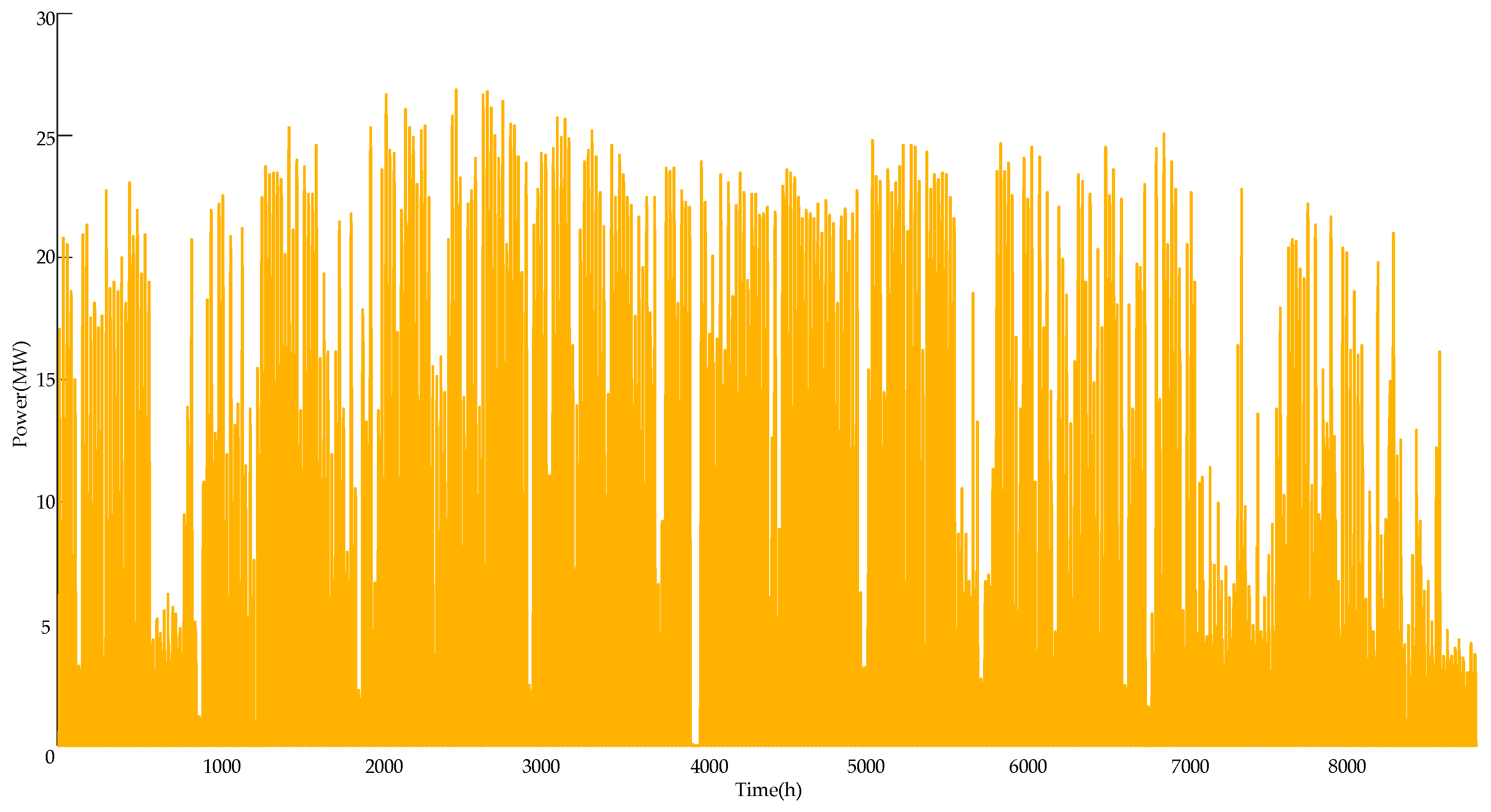
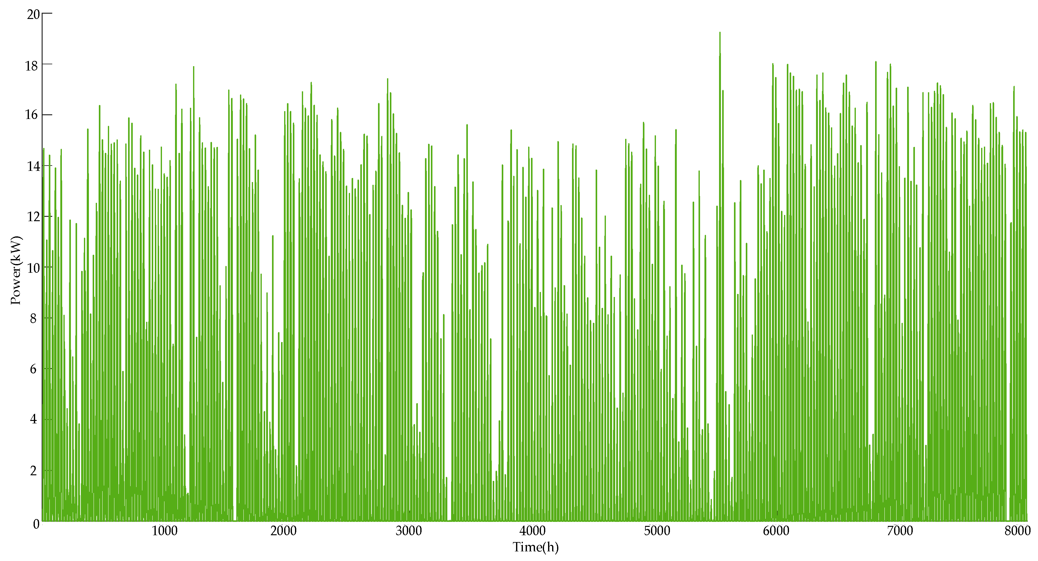
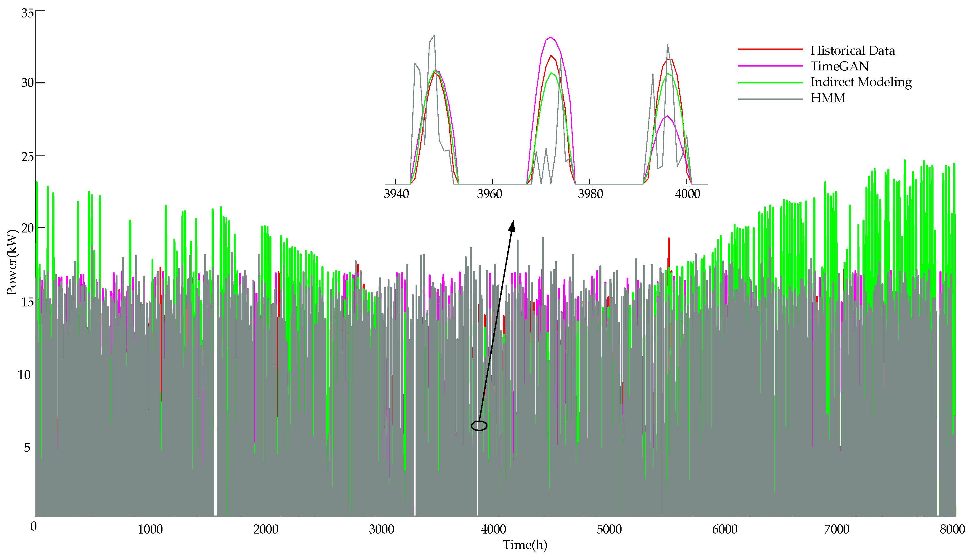
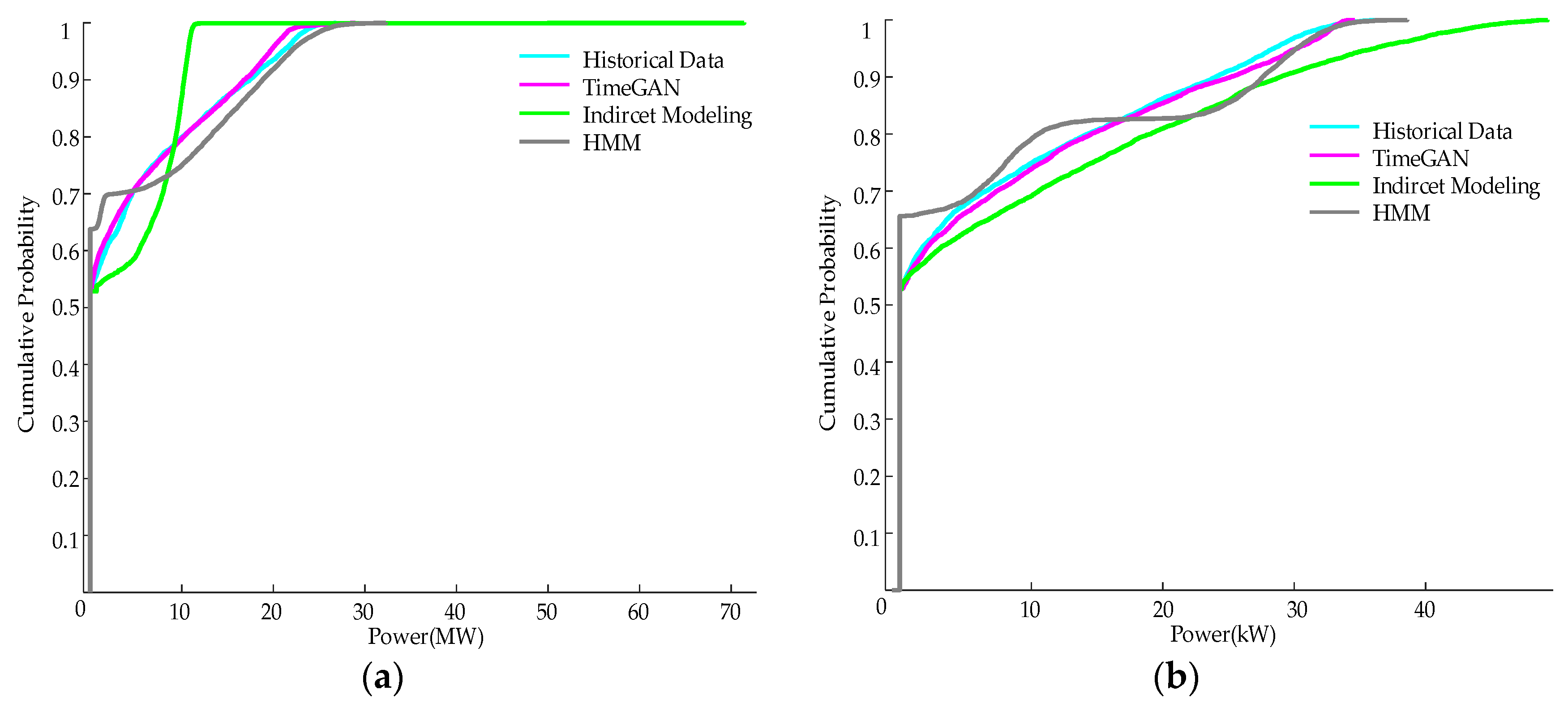
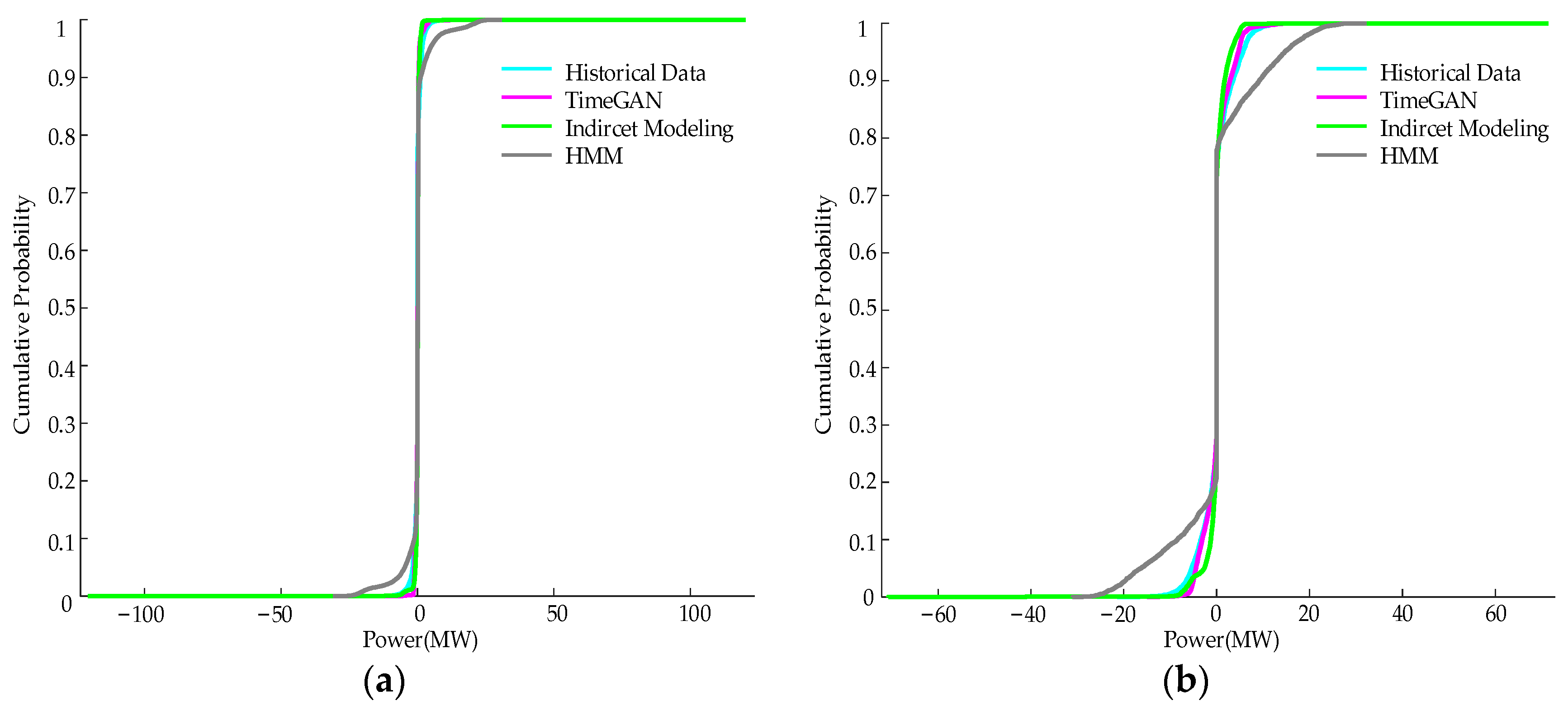
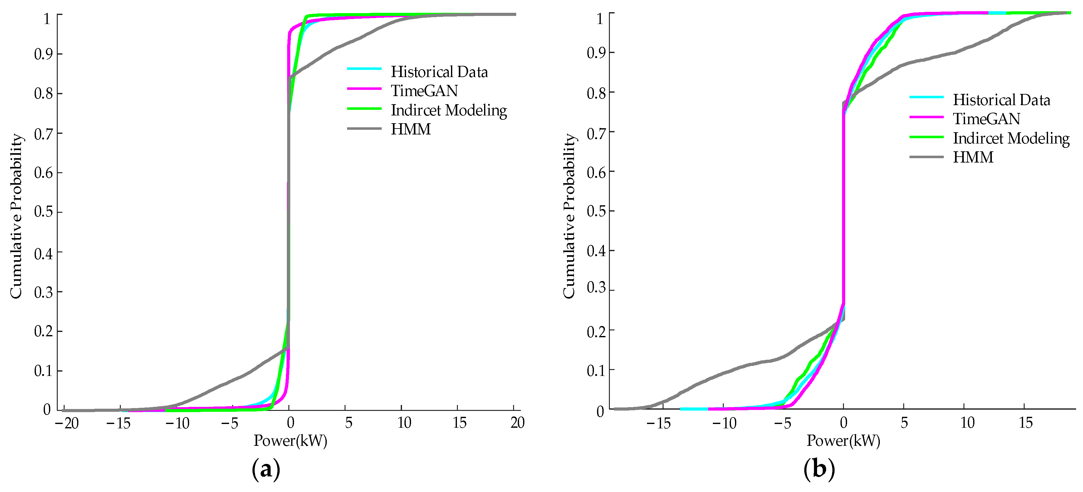
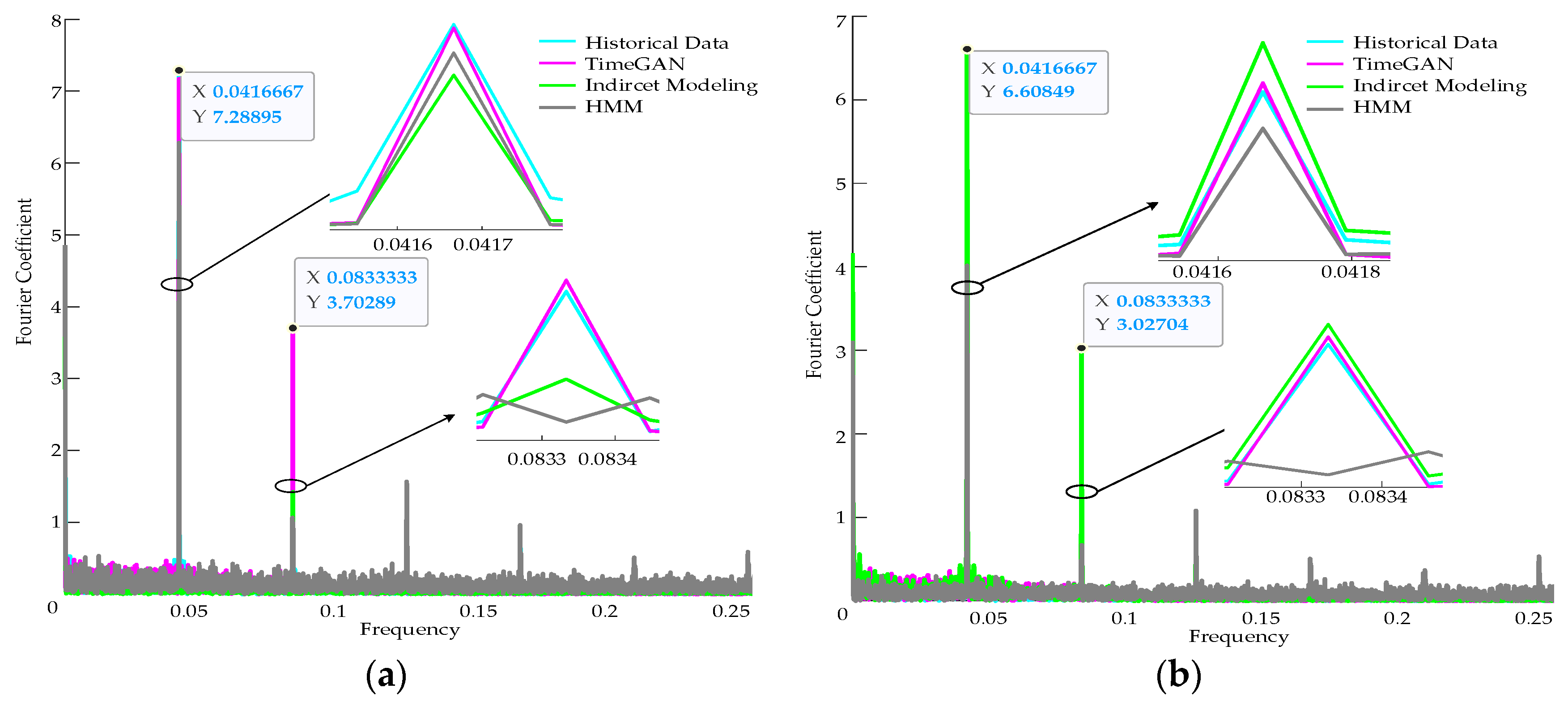
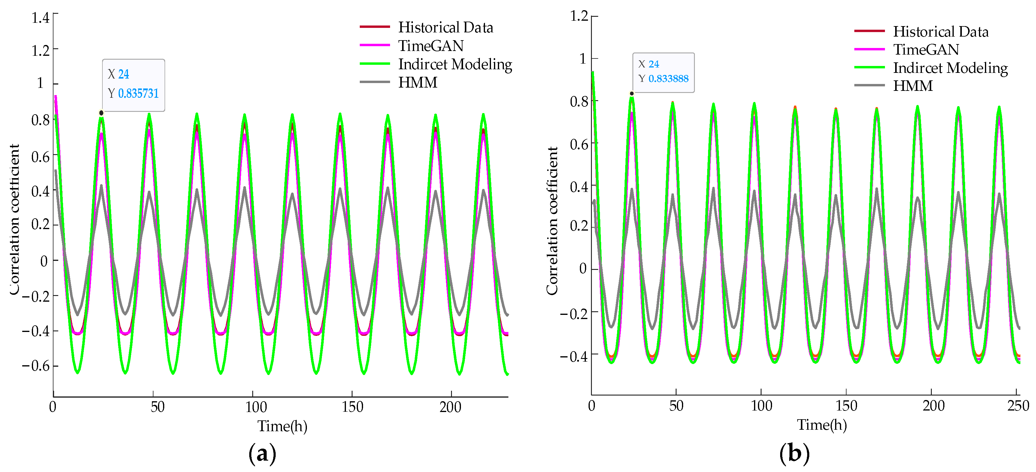
Based on the proposed method, the data of solar power stations in different regions are expanded. The corrected generation data are evaluated from several perspectives, including annual power generation, probability distribution, fluctuation, and periodicity features. The results of the case show that, compared with indirect modeling and HMM, the difference between the annual power generation of solar power data generated via the TimeGAN model and historical data is less than 5%, and the probability distribution curve is closer to the historical data. The error with the maximum fluctuation probability distribution of historical data is within 3%, and it has a better performance in retaining the autocorrelation of the historical data. It shows that the method proposed in this paper has good adaptability to different solar power time-series and is a powerful tool for generating time-series that conform to the statistical characteristics of solar power data.

(3)

Comparing the production cost simulation results of the generated and historical data on the modified IEEE 39-bus system, the error is only 0.25%. It shows that the solar power time-series generated based on the proposed method can support the production cost simulation of new power systems.

However, the TimeGAN model is highly dependent on historical data. In order to obtain higher-quality generated data and reduce the impact of outliers in historical data on the generated data, future work will consider introducing an anomaly detection and repair mechanism into the TimeGAN framework.

References

1. Hu, Q.R.; Guo, Z.S.; Li, F.X. Imitation learning based fast power system production cost minimization simulation. IEEE Trans. Power Syst. 2023, 38, 2951–2954. [Google Scholar] [CrossRef]
2. Jiang, H.; Zhang, H.; Shi, X. Refined production simulation and operation cost evaluation for power system with high proportion of renewable energy. Energy Rep. 2022, 8, 108–118. [Google Scholar] [CrossRef]
3. Liang, C.; Meng, J.; Chen, C.; Zhou, Y. A production-cost-simulation-based method for optimal planning of the grid interconnection between countries with rich hydro energy. Glob. Energy Interconnect. 2022, 3, 23–29. [Google Scholar] [CrossRef]
4. Wang, G.N.; Zhou, T.; Xu, T.S.; Liu, S.F.; Zhang, J.; Chang, K.; Liu, H.T.; Wang, M.X.; Zhang, H.T. Assessment method of new energy real-time accommodation capacity considering uncertainty and power system security constraints. In Proceedings of the 12th International Conference on Power and Energy Systems (ICPES), Guangzhou, China, 23–25 December 2022; pp. 854–859. [Google Scholar]
5. Liu, C.; Huang, Y.; Shi, W.; Li, X. Production Simulation of New Energy Power System, 1st ed.; China Electric Power Press: Beijing, China, 2019; pp. 4–7. [Google Scholar]
6. Wu, Z.; Pan, F.; Li, D.; He, H.; Zhang, T.; Yang, S. Prediction of photovoltaic power by the informer model based on convolutional neural network. Sustainability 2022, 14, 13022. [Google Scholar] [CrossRef]
7. Liu, R.H.; Wei, J.C.; Sun, G.P.; Muyeen, S.M.; Lin, S.F.; Li, F. A short-term probabilistic photovoltaic power prediction method based on feature selection and improved LSTM neural network. Electr. Power Syst. Res. 2022, 210, 108069. [Google Scholar] [CrossRef]
8. Mekhilef, S.; Noraisyah, M.S. Review on the application of photovoltaic forecasting using machine learning for very short- to long-term forecasting. Sustainability 2023, 15, 2942. [Google Scholar]
9. Xia, L.F.; Li, J.M.; Zhao, L.; A1, X.M.; Fanf, J.K.; Wen, J.Y.; Xie, H.L. A PV power time series generating method considering temporal and spatial correlation characteristics. Proc. CSEE 2017, 37, 1982–1993. [Google Scholar]
10. Li, P.; Liu, C.; Huang, Y.H.; Wang, W.S.; Li, Y.H. Modeling correlated power time series of multiple wind farms based on Hidden Markov Model. Proc. CSEE 2019, 39, 5683–5691+5896. [Google Scholar]
11. Kaplani, E.; Kaplanis, S. A stochastic simulation model for reliable PV system sizing providing for solar radiation fluctuation. Appl. Energy 2012, 97, 970–981. [Google Scholar] [CrossRef]
12. Durrani, S.P.; Balluff, S.; Wurzer, L.; Krauter, S. Photovoltaic yield prediction using an irradiance forecast model based on multiple neural networks. J. Mod. Power Syst. Clean Energy 2018, 6, 255–267. [Google Scholar] [CrossRef]
13. Li, P.D.; Gao, X.Q.; Li, Z.C.; Zhou, X.Y. Effect of the temperature difference between land and lake on photovoltaic power generation. Renew. Energy 2022, 185, 86–95. [Google Scholar] [CrossRef]
14. Mokarram, M.; Aghaei, J.; Mokarram, M.J.; Mendes, G.P.; Mohammadi-Ivatloo, B. Geographic information system-based prediction of solar power plant pro duction using deep neural networks. IET Renew. Power Gener. 2023, 17, 2663–2678. [Google Scholar] [CrossRef]
15. Kusznier, J. Influence of environmental factors on the intelligent management of photovoltaic and wind sections in a hybrid power plant. Energies 2023, 16, 1716. [Google Scholar] [CrossRef]
16. Zhou, N.R.; Zhou, Y.; Gong, L.H.; Jiang, M.L. Accurate prediction of photovoltaic power output based on long short-term memory network. IET Optoelectron. 2020, 14, 399–405. [Google Scholar] [CrossRef]
17. Nelega, R.; Greu, D.I.; Jecan, E.; Rednic, V.; Zamfirescu, C.; Puschita, E.; Turcu, R.V.F. Prediction of power generation of a photovoltaic power plant based on neural networks. IEEE Access 2023, 11, 20713–20724. [Google Scholar] [CrossRef]
18. Wang, X.; Wang, Y.; Wang, S.Y.; Shang, K.X.; Su, D.; Cheng, Z.H. A Combination method for PV output prediction using artificial neural network. In Proceedings of the 2021 IEEE IAS Industrial and Commercial Power System ASIA (IEEE I&CPS ASIA 2021), Chengdu, China, 18–21 July 2021; pp. 205–211. [Google Scholar]
19. Xu, M.L.; Ma, C.; Han, X.J. Influence of different optimization aalgorithms on prediction accuracy of photovoltaic output power based on BP neural network. In Proceedings of the 2022 41st Chinese Control Conference (CCC), Hefei, China, 25–27 July 2022; pp. 7275–7278. [Google Scholar]
20. Sansa, I.; Boussaada, Z.; Mrabet-Bellaaj, N. Solar radiation prediction using a novel hybrid model of ARMA and NARX. Energy 2021, 14, 6920. [Google Scholar] [CrossRef]
21. Li, Q.; Zhou, W.; Xia, X. Estimate and characterize PV power at demand-side hybrid system. Appl. Energy 2018, 218, 66–77. [Google Scholar] [CrossRef]
22. Nguyen, R.; Yang, Y.; Tohmeh, A.; Yeh, H.G.H. Predicting PV power generation using SVM regression. In Proceedings of the 2021 IEEE Green Energy and Smart Systems Conference (IGESSC), Long Beach, CA, USA, 1–2 November 2021; pp. 1–5. [Google Scholar]
23. Kong, H.; Sui, H.; Zhang, P. PV Prediction based on PSO-GS-SVM Hybrid Model. In Proceedings of the Joint 2019 International Conference on Ubiquitous Power Internet of Things (UPIOT 2019), Chongqing, China, 21–23 August 2019; p. 012028. [Google Scholar]
24. Xue, J.; Cai, D.; Zhou, G. Application of support vector machines in photovoltaic power prediction. In Proceedings of the 14th International Conference on Intelligent Human-Machine Systems and Cybernetics (IHMSC), Hangzhou, China, 20–21 August 2022; pp. 56–59. [Google Scholar]
25. Yu, L.; Chen, X.; Guo, L. Photovoltaic power prediction method based on Markov Chain and combined model. In Proceedings of the 2021 IEEE International Conference on Power Electronics, Computer Applications (ICPECA), Shenyang, China, 22–24 January 2021; pp. 21–25. [Google Scholar]
26. Zhao, J.; Liu, T.; Kou, Z. Research on prediction model and method of power output of photovoltaic power plant based on neural network and Markov Chain. In Proceedings of the 32nd Chinese Control and Decision Conference (CCDC), Hefei, China, 22–24 August 2020; pp. 2398–2402. [Google Scholar]
27. Zargar, R.H.M.; Yaghmaee Moghaddam, M.H. Development of a markov-chain-based solar generation model for smart microgrid energy management system. IEEE Trans. Sustain. Energy 2020, 11, 736–745. [Google Scholar] [CrossRef]
28. Wu, J. Optimal Dispatch of Micro Grid Economy Considering Uncertainty of Wind Power Photovoltaic Output. Master’s Thesis, Nanjing University of Posts and Telecommunications, Nanjing, China, 2020. [Google Scholar]
29. Wang, Z.; He, L.; Ding, G. Short term power generation combination prediction based on EMD-LSTM-ARMA model. Mod. Electr. Trans. 2023, 46, 151–155. [Google Scholar]
30. Tagliaferri, F.; Hayes, B.P.; Viola, I.M.; Djokic, S.Z. Wind modelling with nested Markov chains. J. Wind Eng. Ind. Aerodyn. 2016, 157, 118–124. [Google Scholar] [CrossRef]
31. Soares, T.G.; Lima, F.J.L.; Martins, F.R. Generating solar irradiance data series with 1-minute time resolution based on hourly observational data. IEEE Lat. Am. Trans. 2021, 19, 191–198. [Google Scholar]
32. Ma, M.; Ye, L.; Li, J.; Li, P.; Song, R.; Zhuang, H. Photovoltaic time series aggregation method based on K-means and MCMC algorithm. In Proceedings of the 2020 12th IEEE PES Asia-Pacific Power and Energy Engineering Conference (APPEEC), Nanjing, China, 20–23 September 2020; pp. 1–6. [Google Scholar]
33. Jiang, X.; Zhu, J.; Yuan, Y.; Wang, Y.; Huang, R. PV output time series simulation method based on new scenario division and considering time series correlation. Electr. Power Cons. 2018, 39, 63–70. [Google Scholar]
34. Creswell, A.; White, T.; Dumoulin, V.; Arulkumaran, K.; Sengupta, B.; Bharath, A.A. Generative adversarial networks an overview. IEEE Signal Proc. Mag. 2018, 35, 53–65. [Google Scholar] [CrossRef]
35. Goodfellow, I.; Pouget-Abadie, J.; Mirza, M.; Xu, B.; Warde-Farley, D.; Ozair, S.; Courville, A.; Bengio, Y. Generative adversarial networks. Commun. ACM 2020, 63, 139–144. [Google Scholar] [CrossRef]
36. Aggarwal, A.; Mittal, M.; Battineni, G. Generative adversarial network: An overview of theory and applications. Int. J. Inf. Manag. Data Insights 2021, 1, 100004. [Google Scholar] [CrossRef]
37. Banat, R.; Colton, S. Autoregressive self-evaluation: A case study of music generation using large language models. In Proceedings of the IEEE Conference on Artificial Intelligence (IEEE CAI), Santa Clara, CA, USA, 5–6 June 2023; pp. 264–265. [Google Scholar]
38. Hsu, P.C.; Liu, D.R.; Liu, A.T.; Lee, H.Y. Parallel synthesis for autoregressive speech generation. IEEE-ACM Trans. Audio Speech Lang. Process. 2023, 31, 3095–3111. [Google Scholar] [CrossRef]
39. Duran, N.; Catak, M. Forecasting of wind speed by means of window-shifted autoregressive time series. In Proceedings of the 24th Signal Processing and Communication Application Conference (SIU), Zonguldak, Turkey, 16–19 May 2016; pp. 2149–2151. [Google Scholar]
40. Jinsung, Y.; Daniel, J.; Mihaela, S. Time-series generative adversarial networks. NeurlPS Proc. 2019, 32, 5508–5518. [Google Scholar]
41. Deng, W.; Dai, Z.; Liu, X.; Chen, R.; Wang, H.; Zhou, B.; Tian, W.; Lu, S.; Zhang, X. Short-Term wind power prediction based on wind speed interval division and TimeGAN for gale weather. In Proceedings of the International Conference on Power Energy Systems and Applications, Nanjing, China, 24–26 February 2023; pp. 352–357. [Google Scholar]
42. Zhang, Y.; Zhou, Z.; Liu, J.; Yuan, J. Data augmentation for improving heating load prediction of heating substation based on TimeGAN. Energy 2022, 260, 124919. [Google Scholar] [CrossRef]
43. Li, Q.; Zhang, X.Y.; Ma, T.J.; Liu, D.G.; Wang, H.; Hu, W. A Multi-step ahead photovoltaic power forecasting model based on TimeGAN, Soft DTW-based K-medoids clustering, and a CNN-GRU hybrid neural network. Energy Rep. 2022, 8, 10346–10362. [Google Scholar] [CrossRef]
44. Zhang, Y.S. Research on Key Technologies of Remaining Useful Life Estimation for Industrial Equipment Based on Deep Learning. Master’s Thesis, University of Electronic Science and Technology of China, Chengdu, China, 2022. [Google Scholar]
45. Su, J. Several mathematical models for calculating moonrise, sunrise and sunset time. Mod. Vocat. Educ. 2016, 34, 38–39. [Google Scholar]
46. Jing, C.G.; Shu, D.M.; Gu, D.Y. Implementation of sunrise and sunset time algorithm in urban street lamp monitoring system. Mod. Comput. 2003, 5, 84–86. [Google Scholar]
47. Gao, S.P. Wind/Photovoltaic Power Time Series Generation and Scenarios Reduction Methods for Power System Planning. Master’s Thesis, Chongqing University, Chongqing, China, 2021. [Google Scholar]
Figure 1. Structure diagram of solar power data generation model based on TimeGAN.
Sustainability 15 14920 g001
Figure 2. Training process of the solar power data generation model based on TimeGAN.
Sustainability 15 14920 g002
Figure 3. Historical solar power data of Station 1.
Sustainability 15 14920 g003
Figure 4. Historical solar power data of Station 2.
Sustainability 15 14920 g004
Figure 5. Historical and generated solar power time-series of Station 1.
Sustainability 15 14920 g005
Figure 6. Historical and generated solar power time-series of Station 2.
Sustainability 15 14920 g006
Figure 7. (a) Probability distribution of Station 1. (b) Probability distribution diagram of Station 2.
Sustainability 15 14920 g007
Figure 8. (a) 15 min maximum fluctuation probability distributions of Station 1; (b) 1 h maximum fluctuation probability distributions of Station 1.
Sustainability 15 14920 g008
Figure 9. (a) 15 min maximum fluctuation probability distributions of station 2; (b) 1 h maximum fluctuation probability distributions of station 2.
Sustainability 15 14920 g009
Figure 10. (a) Fourier coefficient–frequency diagram of Station 1; (b) Fourier coefficient–frequency diagram of Station 2.
Sustainability 15 14920 g010
Figure 11. (a) Autocorrelation coefficient diagram of Station 1; (b) Autocorrelation coefficient diagram of Station 2.
Sustainability 15 14920 g011