Article

The Effects of Local Government Expenditures on Carbon Dioxide Emissions: Evidence from Republic of Korea

College of Business, Gachon University, Seongnam-si 13120, Gyeoggi-do, Republic of Korea
Sustainability 2023, 15(20), 14913; https://doi.org/10.3390/su152014913
Submission received: 31 July 2023 / Revised: 4 October 2023 / Accepted: 12 October 2023 / Published: 16 October 2023
(This article belongs to the Section Social Ecology and Sustainability)

Abstract

:
This study analyzes the direct and indirect effects of local government expenditure for air quality on CO2 emissions using a two-stage dynamic panel model. The results of the first-stage empirical analysis show that local government expenditure for air quality has a positive effect on per-capita GRDP. In the second-stage empirical analysis, an inverse U-shaped relationship between the per-capita GRDP and CO2 emissions is observed. The average direct and indirect effects of local government expenditure for air quality on CO2 emissions indicate that local government expenditure directly reduces CO2 emissions, while it indirectly increases CO2 emissions through regional economic growth. However, the direct effect is found to be greater than the indirect effect, and the total effect indicates that local government expenditure for air quality reduces CO2 emissions. Furthermore, the results demonstrate significant regional disparities in both the direct and indirect effects, emphasizing the pivotal role of tailored air-related expenditure policies in relation to regional economic growth.

1. Introduction

South Korea has significantly ramped up its fiscal spending on environmental initiatives to tackle escalating environmental challenges. According to the Bank of Korea, from 2008 to 2018, South Korea’s real gross domestic product (GDP) surged impressively by about 36.7%, skyrocketing from KRW 1325 trillion (approximately USD 1.05 trillion) to KRW 1812 trillion (about USD 1.73 trillion) [1]. This economic boom, however, paralleled a concerning spike in greenhouse gas emissions, surging by 22.5% from 594 million tons to 728 million tons [2]. To reduce the greenhouse gas emissions resulting from this economic growth, South Korea has set an ambitious target to slash national greenhouse gas emissions by 37% (equivalent to 315 million tons of CO2eq.) compared with the business-as-usual level of 851 million tons CO2eq. by 2030. To achieve this goal, both central and local governments have devised region-specific policies for greenhouse gas reduction, bolstering their financial commitments to addressing environmental concerns. Governmental policy intervention has emerged as a crucial catalyst in mitigating environmental challenges and enhancing environmental quality [3,4,5].
Environmental quality aligns with the characteristics of a public good, which justifies government intervention and expenditure to attain an appropriate level of environmental quality. In 1995, South Korea implemented the local autonomy system, transferring environmental policies and administration from the central government to local governments. Presently, while local governments predominantly spend fiscal expenditures related to the environment, their role in government spending to combat environmental issues has become increasingly significant [6]. To meet environmental policy objectives, a comprehensive assessment and discussion of environmental budgets has taken place. This process has not only assisted local governments in effectively addressing environmental concerns, but has also become vital for validating policy goals and shaping future plans. However, despite these efforts, little attention has been given to analyzing whether local government expenditures in the environmental sector have genuinely contributed to enhancing environmental quality.
Concerning the impact of government expenditures on environmental quality, it is important to pay attention to the relationships among three factors: government expenditure, economic growth, and environmental quality. In economics, there is a theoretical background regarding the relationship between government expenditure and economic growth. Since gross domestic product is measured by the sum of consumption, investment, government expenditure, and net exports, it is well-known that government expenditure is linked to promoting economic growth [7,8,9]. Regarding the linkage between economic growth and regional environmental quality, it has been explored through the environmental Kuznets curve (EKC) hypothesis [10,11]. According to the EKC hypothesis, in the initial phases of economic growth, there tends to be a focus on expanding the economy at the expense of environmental considerations. However, when the economy attains a specific income level, the quality of the environment starts to ameliorate due to a notable uptick in environmental consciousness, regulations, and technological innovations to address pollution and resource depletion. Moreover, concerning the linkage between local fiscal expenditure and environmental concerns, theoretical insights are provided into the ways government expenditure can impact the quality of the environment.
However, there is a lack of studies that have examined the effects of environment-related expenditure on environmental quality, considering the nexus of government expenditure, economic growth, and carbon dioxide (CO2) emissions. Previous studies have individually examined the effects of fiscal expenditure on economic growth, the effects of economic growth on CO2 emissions, and the effects of fiscal expenditure on CO2 emissions. If there are significant relationships among government expenditure, economic growth, and CO2 emissions, it is possible to observe both the direct effect of government expenditure on CO2 emissions (i.e., local government expenditure CO2 emissions) and the indirect effect of government expenditure on economic growth, subsequently influencing CO2 emissions (i.e., local government expenditure local economic growth CO2 emissions).
Thus, this study focuses on analyzing the direct and indirect impacts of air-related financial expenditure on CO2 emissions, employing a two-stage dynamic panel method. The first stage examines the impact of government expenditures for air quality by region on the gross regional domestic product (GRDP), taking into account the endogeneity of GRDP variables. Building upon the results of the first-stage analysis, the second stage investigates the influence of both GRDP and air-related expenditure on CO2 emissions. From the first and second stages, this study separately evaluates the direct and indirect effects of government expenditures for air quality on CO2 emissions. Moreover, this study contributes to the literature by identifying the direct and indirect effects across local regions with different GRDP levels. The detailed research hypotheses are as follows.
H1. 
Local government expenditure for air quality enhances local economic growth.
H2. 
There is an inverted U-shaped curve between GRDP and CO2 emissions.
H3. 
Local air-related expenditure reduces CO2 emissions.
H4. 
There are varying direct and indirect effects across local regions with different GRDP levels.
The structure of this study is as follows. Section 2 and Section 3 provide a literature review and an introduction to the data utilized in the empirical analysis, as well as an overview of the two-step dynamic panel method. Section 4 and Section 5 present the analysis findings, conclusions, and their implications.

2. Literature Review

Many studies have highlighted the crucial role of the government’s fiscal expenditure not only in affecting economic growth, but also in addressing environmental problems. In this section, we review the existing studies concerning three relationships: the effects of government expenditure on economic growth, the impact of economic growth on environmental quality, and the effects of government expenditure on environmental quality, with a focus on CO2 emissions.

2.1. Impact of Government Expenditure on Economic Growth

There is a theoretical background about the relationship between government expenditure and economic growth. The Keynesian theory highlights the role of government expenditure in promoting economic growth [7]. As the gross domestic product (GDP), a key macroeconomic indicator of economic growth, is composed of consumption, investment, government expenditure, and net exports, the portion of government expenditure used for purchasing final goods and services is directly incorporated into GDP. On the other hand, classical and neoclassical economists have emphasized that government expenditures affect economic growth negatively [8,9]. When the size of the government expands, owing to the distortionary effects of taxation, the level of inefficiency within the government is likely to increase. This, in turn, indicates that government expenditures impede economic growth. To validate this hypothesis, a comprehensive range of empirical analysis studies have been conducted.
The empirical findings of studies analyzing the relationship between government expenditure and economic growth are controversial. Some studies suggest a positive effect of government expenditure on regional economic growth [12,13,14,15,16,17]. These studies show that government expenditure generally enhances the productivity of private capital and investment, thereby exerting a positive influence on long-term economic growth. Most studies have found a positive effect in the relationship between government expenditure and economic growth, although a few studies have produced varied results across countries and time periods [18,19,20,21,22,23,24,25]. For instance, according to Sáez et al. [23], the effects of government expenditure on economic growth varied across countries. Positive effects have been observed in countries such as Portugal, the United Kingdom, France, Greece, and Luxembourg, while negative effects have been found in countries such as Austria, Germany, Denmark, Finland, Italy, and Sweden. In addition, Frank et al. [20] found positive effects in the long term, but negative effects in the short term, while Ajayi and Aluko [22] did not establish any significant relationship between government expenditure and economic growth.
On the other hand, contrasting views have also been presented, which indicate negative effects of government expenditure on economic growth [26,27,28,29,30,31]. The negative impact implies that productivity in the governmental sector may be lower than that in the private sector, or economic leakage may have a detrimental impact on economic growth. The effectiveness of government expenditure can also be influenced by sector-specific productivity differences or potential economic leakage. For example, Gwartney et al. [26] emphasized that, as the size of the government expands, it starts having a negative impact on economic growth beyond a certain threshold, suggesting the need to reduce government expenditure. Muhammad et al. [27] also revealed a negative correlation between government expenditure and long-term economic growth. In addition, Bergh and Karlsson [28] and Zimcik [30] emphasized a negative relationship between economic growth and government size when measured as the proportion of taxes to GDP.

2.2. Impact of Economic Growth on Environmental Quality

The relationship between economic growth and regional environmental quality has mainly been investigated through the environmental Kuznets curve (EKC) hypothesis [10,11]. The EKC hypothesis indicates that, during the early stages of economic growth, there is a tendency to prioritize economic expansion over environmental concerns, resulting in increased resource consumption, pollution, and environmental degradation [32]. However, as countries achieve a certain level of income or economic development, and after reaching a certain economic threshold, environmental awareness escalates, regulations become more stringent, and technological advancements are made to mitigate pollution and resource exploitation. Consequently, the quality of the environment begins to improve as the economy grows. Therefore, when applying the EKC hypothesis to the relationship between CO2 emissions and economic growth, there is an inverted U-shaped curve between CO2 emissions and economic growth. Initially, as economic growth progresses, CO2 emissions tend to deteriorate, but after reaching a certain level of income, CO2 emissions start to improve.
In studies analyzing the relationship between CO2 emissions and economic growth based on the EKC hypothesis, there are lots of findings of inverted U-shaped curves, indicating that environmental quality improves with economic growth [33,34,35,36,37]. For example, Sharfik [33] observed a continuous increase in CO2 emissions as income rises. Some studies discovered that renewable energy contributes to a decrease in CO2 emissions [34,35,36,37]. On the other hand, the extensive studies of Allard et al. [38] and Fang et al. [39] identified an inverted N-shaped curve, while Abdallah et al. [40] found an N-shaped curve.
With a focus on Korea, some studies identified an inverted U-shaped relationship between the two variables [41,42,43,44,45,46], whereas other studies could not find a relationship [47]. In the studies of Lee and Li [41] and Lee [43], it was confirmed that the EKC hypothesis held, while an increase in energy prices was found to contribute to the reduction in CO2 emissions. In addition, Choi et al. [42] examined the relationship between CO2 emissions, economic growth, and economic openness, validating the EKC hypothesis, and Kim and Jung [46] discovered an inverted U-shaped relationship when considering total factor productivity. Kim and Kim [44] verified the EKC relationship and found that an increase in electricity consumption could lead to an increase in CO2 emissions, while an increase in renewable energy generation could decrease CO2 emissions.

2.3. Impact of Government Expenditure on Environmental Quality

Regarding the relationship between local fiscal expenditure and environmental issues, Lopez et al. [48] and Halkos and Paizanos [49] theoretically explained the reasons why the quality of the environment could be influenced by government expenditures, discussing four effects: the scale, composition, technique, and income effects. The scale effect suggests that economic growth could intensify environmental pressures, leading to an increase in government expenditures, and the composition effect indicates that environmental quality could be compromised due to human activities resulting from the accumulation of human capital. The technique effect implies that higher labor productivity might result in greater demand for government expenditure in the environmental sector, while the income effect means that rising income could drive heightened concern for environmental quality, elevating the demand for government expenditure. These four effects are useful to manifest differently depending on the type of pollutants, and the impacts of government expenditures on the environment could exhibit varying patterns, depending on specific pollutants or regions.
Several studies have examined it by incorporating environmental fiscal expenditure with CO2 emissions [31,49,50,51,52,53,54]. Halkos and Paizanos [49] estimated the direct and indirect effects of government expenditure on CO2 emissions. While they did not find statistically significant results for the direct effect of government expenditure on CO2 emissions, they obtained a negative value for the indirect effect. In addition, Halkos and Paizanos [52] reported that expansionary fiscal spending would lead to the alleviation of CO2 emissions, whereas contractionary fiscal spending, due to increased consumption resulting from tax cuts, would lead to an increase in CO2 emissions. Adewuyi [53] discovered a positive significant impact of government expenditure on CO2 emissions in the long run, but a negative effect in the short run. Zhang et al. [31] estimated the effects on three pollutants (SO2, COD, and soot) and found that indirect effects from government expenditure played a crucial role in determining the total effects on these pollutants. Furthermore, Fan et al. [54] revealed that disparities in government expenditure structure were the primary contributors to CO2 emissions inequality. Recent studies by Jin et al. [55] demonstrated that green R&D expenditure enhanced environmental quality, whereas Erdogan et al. [56] and Pata et al. [57] emphasized the roles of renewable energy in reducing CO2 emissions.
As a study specifically focused on Korea, there is a lack of research that has clearly examined the relationship between government expenditure and environmental quality. Kwon et al. [6] investigated the impact of financial expenditure in the environmental field by considering fine dust, ozone, and nitrogen dioxide as measures of environmental quality. They found that government expenditure did not alleviate the emissions of air pollutants, suggesting that government expenditure would not be effectively implemented. Furthermore, there is a lack of studies that have examined the relationship between government expenditure and environmental quality, reflecting the contribution of government expenditure to economic growth. From the literature review, we can find a potential relationship among government expenditure, economic growth, and environmental quality; thus, it is necessary to conduct an integrative analysis to clearly identify the relationships among three factors to suggest more detailed policy implications.

3. Materials and Methods

3.1. Data

The empirical analysis includes 16 cities and provincial regions for the period from 2008 to 2018. Table 1 presents the basic statistics of the variables for the empirical analysis. The gross regional domestic product (GRDP) data were obtained from the Regional Income Dataset provided by Statistics Korea, while the data for fiscal expenditure (AEXP) were derived from the Local Finance Yearbook (The Local Finance Yearbook is a compilation of fiscal indicators and statistics provided by the Ministry of the Interior and Safety in South Korea. It offers financial indicators and statistics of local governments, including budget, revenue, expenditure, debt, and more. This enables an understanding of the financial situation and trends of each local government. Also, the Local Finance Yearbook provides annual data on environmental protection expenditures by local governments, including water quality, waste, air quality, nature, marine, etc.) published by the Ministry of the Interior and Safety [1,58]. The variables were adjusted by dividing them by the consumer price index and the population count to express them in real values per person. The CO2 emissions data by region were sourced from the Greenhouse Gas Inventory and Research Center of the Ministry of Environment [2]. Additionally, the data for labor (LABOR) utilized the number of individuals employed, as obtained from the Economically Active Population Survey conducted by Statistics Korea. As for the capital variable (CAPITAL), the year-end balance of tangible assets, excluding land, obtained from the Mining and Manufacturing Survey provided by Statistics Korea was used as a proxy variable [59]. For the energy variable (ENERGY), the data from the Regional Energy Statistical Yearbook published by the Korea Energy Economics Institute were utilized [60]. The data for industrial area (INDUSTRY) were derived from the Urban Planning Status provided by the Korea Land & Housing Corporation [61]. Moreover, to account for the influence of price variables in estimating the environmental Kuznets curve (EKC), the energy price index (EPI) was included as an explanatory variable, following the approach of Agras and Chapman [62]. The energy price index was constructed using the price index for electricity, gas, and other fuels sourced from the Consumer Price Survey by Statistics Korea [59]. The energy price index was calculated by applying the weight for each item of the consumer price index as of 2020.
Figure 1 illustrates the average values of per-capita GRDP and per-capita CO2 emissions by region for the 2008–2018 period. A higher GRDP per capita is observed in Ulsan, Chungnam, and Jeonnam, with values of KRW 59.49 million, KRW 44.95 million, and KRW 36.54 million, respectively, whereas Daegu, Gwangju, and Busan have lower GRDP per capita, with values of KRW 18.97 million, KRW 10,000, and KRW 21.86 million, respectively. In terms of CO2 emissions per capita, Chungnam (67.3 t), Ulsan (36.8 t), and Jeonnam (47.3 t) exhibited higher levels due to their status as industrial cities with significant energy consumption from sectors such as coal-fired power generation, petrochemicals, steel, and shipbuilding. On the other hand, Seoul, Gwangju, and Daegu record lower CO2 emissions per capita, with values of 3.1 tons, 3.6 tons, and 3.7 tons, respectively.
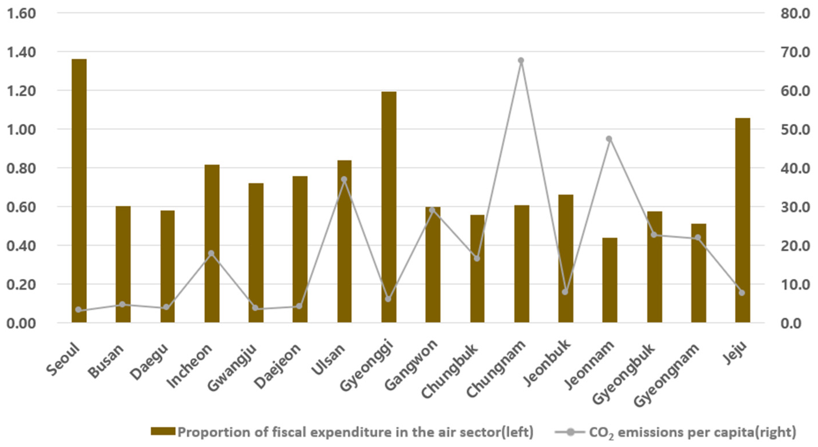
In Figure 2, the proportion of fiscal expenditure for air quality relative to total local government expenditure ranges from 0.44% to 1.36% across the 16 regions. Among them, Seoul has the highest proportion at 1.36%, followed by Gyeonggi (1.19%), and Jeju (1.05%), while the proportions are lower in Chungnam (0.60%), Ulsan (0.84%), and Jeonnam (0.44%). The Seoul, Gyeonggi, and Jeju regions exhibit a higher proportion of fiscal expenditure for air quality compared with their relatively low CO2 emissions. However, regions with high CO2 emissions, such as Chungnam, Jeonnam, and Ulsan, show a slightly lower proportion of fiscal expenditure for air quality.

3.2. Methodology

This study adopts two-stage dynamic panel analysis, building upon the research conducted by Cole [63] and Halkos and Paizanos [49], to examine the direct and indirect effects of financial expenditure for air quality on CO2 emissions. In the first step, the analysis focuses on assessing the impact of fiscal expenditure for air quality on the GRDP. In the second step, this study estimates the influence of fiscal expenditure and GRDP on CO2 emissions using the fitted value of the GRDP. For the empirical analysis, the dynamic panel model is employed and estimated using the generalized method of moments (GMM) approach developed by Hansen [64] and Arellano and Bond [65]. In the first stage of analysis, Equation (1) is estimated to analyze the impact of financial expenditure for air quality on the per-capita GRDP.
ln G R D P i t = α 0 ln G R D P i t 1 + α 1 ln A E X P i t + α 2 ln Z i t + μ i + δ t + ϵ i t
where the dependent variable ( G R D P i t ) represents the per-capita GRDP of region i in year t , while the explanatory variable ( A E X P i t ) denotes fiscal expenditure for air quality of region i in year t . Equation (1) incorporates a first-order-lagged variable as an explanatory variable, and additional variables, such as labor, capital, and energy consumption ( Z i t ), are considered as additional explanatory factors. In addition, μ i represents the individual effect of region i , δ t represents the time effect, and the error term ϵ i t assumes independent and identically distributed (i.i.d) properties.
In the second-stage analysis, the model depicted in Equation (2) is utilized to examine the effects of fiscal expenditure and GRDP on CO2 emissions.
ln C O 2 i t = β 0 ln C O 2 i t 1 + β 1 E ln G R D P i t + β 2 E ln 2 G R D P i t + β 3 ln A E X P i t + β 4 ln X i t + θ i + γ t + u i t
where the dependent variable ( C O 2 i t ) represents CO2 emissions per capita in region i in year t . Equation (2) includes ( C O 2 i t 1 ), a first-order lag variable, as an explanatory variable. E l n G R D P i t denotes the estimated value of GRDP, while the other explanatory variables ( X i t ) include labor, capital, energy consumption, industrial area, and the energy price index. To capture the non-linear relationship between CO2 emissions and GRDP, explanatory variables in the form of squares of GRDP are included in Equation (2). Similar to Equation (1), θ i represents the individual effect of region i , γ t denotes the time effect, and the error term u i t is assumed to be i.i.d.
According to Cole [63] and Halkos and Paizanos [49], the direct, indirect, and total effects of fiscal expenditure for air quality on CO2 emissions can be computed. The direct effect is estimated in Equation (2), while the indirect effect is the impact of fiscal expenditure on per-capita GRDP in Equation (1) multiplied by the effect of per-capita GRDP on CO2 emissions estimated in Equation (2). In other words, the total effect is calculated by
ln ( C O 2 ) ln ( A E X P ) + ln ( C O 2 ) ln ( G R D P ) · ln G R D P ln A E X P
where the first term indicates the direct effect, while the second term represents the indirect effect. As the total effect is obtained by summing the direct and indirect effects, as indicated in Equation (3), the total effect in terms of the estimates is represented by
T o t a l   E f f e c t = β 3 + α 1 × ( β 1 + β 2 E l n G R D P )
where the direct effect corresponds to the impact of fiscal expenditure on per-capita CO2 emissions, while the indirect effect captures the influence of fiscal expenditure on per-capita CO2 emissions through its impact on per-capita GRDP. In Equation (4), the indirect effect is evaluated for per-capita GRDP across different regions so that the total effect varies with local economic growth.

4. Results

Based on the panel data, a two-stage empirical analysis was conducted to examine the impact of fiscal expenditure for air quality on CO2 emissions using the STATA software. For estimating the empirical model, a comparison was made between the results of the dynamic panel model and those of the static panel model. That is, in addition to the generalized method of moments (GMM) analysis, the analysis involved the estimations using pooled ordinary least squares (POLS) and fixed-effect models. The interpretation of the estimation results primarily focused on the results obtained from the dynamic panel model estimated using the GMM.
Table 2 presents the estimation results of the first-stage analysis. For the valid estimation of the dynamic panel model, the autocorrelation tests show that there were no second-order serial autocorrelation problems due to the p-value of 0.172, while the Hansen J test confirmed that there were no over-identification problems due to the p-value of 0.115. According to the results of the first-stage analysis in Table 2, the estimated coefficient of the lagged variable (lagged per-capita GRDP) is 0.866, which is statistically significant at the 1% level. This indicates that the lagged per-capita GRDP has a positive influence on the current per-capita GRDP, suggesting the presence of dynamic effects in per-capita GRDP. The validity of Keynes’ hypothesis has been established, aligning with the outcomes of prior research. Furthermore, in line with previous studies, it has been demonstrated that government expenditure exerts a positive impact on economic growth [12,13,14,15,16,17].
Regarding fiscal expenditure for air quality (AEXP), a 1% increase in air-related fiscal expenditure is found to contribute to a 0.008% increase in per-capita GRDP. This implies that fiscal expenditure can contribute to regional economic growth. The estimates for labor and capital did not yield statistical significance, whereas it is observed that energy consumption contributed approximately 0.020% to the increase in per-capita GRDP.
Table 3 presents the results of the second-stage empirical analysis, where the fitted values of GRDP from the first-stage analysis are included as explanatory variables to estimate the effects of fiscal expenditure for air quality and GRDP on CO2 emissions. The autocorrelation tests also showed that there were no second-order serial autocorrelation problems due to the p-value of 0.974, while the Hansen J test confirmed that there were no over-identification problems due to the p-value of 0.143. First, the estimate of the lagged variable of CO2 emissions ( C O 2 i t 1 ) was 0.585, which was statistically significant at the 1% level. This indicates the presence of dynamic effects in CO2 emissions. The examination of the EKC relationship between GRDP and CO2 emissions showed a statistically significant inverted U-shaped relationship. That is, the EKC hypothesis between economic growth and CO2 emissions was verified, and as demonstrated in previous studies, a statistically significant inverted U-shaped relationship was identified [33,34,35,36,37]. This means that, as the per-capita GRDP increased, CO2 emissions also increased, but after reaching a turning point, CO2 emissions started to decrease. The turning point was calculated using the formula of exp( β 1 / 2 β 2 ) and suggested that CO2 emissions started decreasing once the per-capita GRDP reached, on average, approximately KRW 39.66 million.
In the case of fiscal expenditure for air quality, the estimated coefficient was found to be −0.017, indicating that a 1% increase in fiscal expenditure led to a reduction in CO2 emissions by 0.017%. The negative effects of such government expenditure on CO2 emissions appeared to be similar to the findings of previous studies [31,49,53]. This suggests that local government expenditure for air quality contributes to economic growth while simultaneously reducing air pollution. Additionally, the increased number of employees was found to have a negative impact on CO2 emissions (−0.409), indicating that industries with higher labor intensity tend to have lower CO2 emissions. Conversely, the increased energy use had a positive impact on CO2 emissions (0.382), suggesting that industries with higher energy intensity tend to have higher CO2 emissions. Moreover, the estimation coefficient for the energy price index was −0.162, indicating that a 1% increase in energy prices results in a decline in CO2 emissions by approximately 0.162%. Relatively higher energy prices seem to reduce CO2 emissions by exerting pressure on energy costs and constraining energy demand.
Based on the estimation results in Table 2 and Table 3, we estimated the direct and indirect effects of fiscal expenditure for air quality on CO2 emissions. When analyzing the average GRDP, the indirect effect was calculated as 0.005, multiplying the effect of fiscal expenditure for air quality on per-capita GRDP ( ln G R D P / l n ( A E X P ) ) by the effect of per-capita GRDP on CO2 emissions ( ln C O 2 / l n ( G R D P ) ). The total effect, combining the direct and indirect effects, was then estimated to be −0.012( = 0.017 + 0.005 ), indicating that fiscal spending for air quality directly decreases CO2 emissions, but indirectly increases CO2 emissions through its contribution to regional economic growth. The direct effect is larger than the indirect effect, suggesting that a rise in fiscal expenditure for air quality leads to a reduction in CO2 emissions.
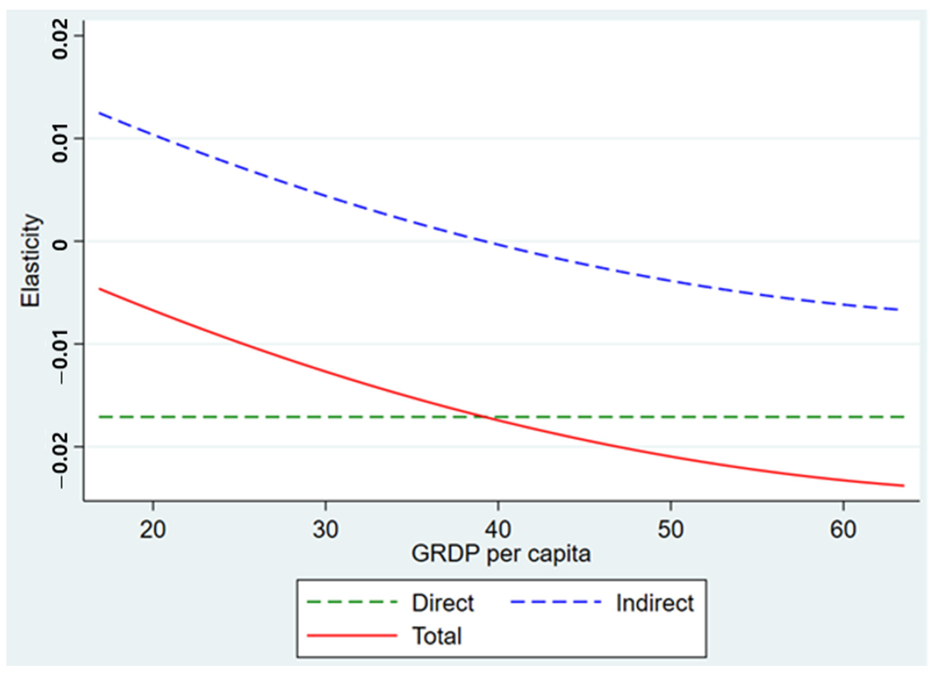
When examining the direct and indirect effects based on different per-capita GRDP levels, they can be visualized as shown in Figure 3. The figure illustrates the direct, indirect, and total effects in terms of elasticities. The direct effect consistently demonstrates a negative (−) value, regardless of per-capita GRDP, whereas the indirect effect exhibits a decreasing trend. Initially, the indirect effect starts with a positive (+) value at low levels of per-capita GRDP, but transitions to a negative (−) value after the per-capita GRDP reaches approximately KRW 39.661 million. Consequently, the total effect shows a decreasing pattern as the per-capita GRDP increases, mirroring the trend of the indirect effect. These results indicate an increase in fiscal expenditure for air quality relative to per-capita GRDP across all levels of per-capita GRDP.
Meanwhile, Table 4 reports the direct, indirect, and total effects by region. The direct effects remained constant at −0.017 across all regions. However, the indirect effects showed positive (+) values for all regions, except for Ulsan and Chungnam. Specifically, the indirect effects for Ulsan and Chungnam were estimated to be −0.006 and −0.002, respectively. The results are attributed to per-capita GRDP levels above the turning point of KRW 39.66 million. In the cases of Ulsan and Chungnam, the indirect effects were derived as negative (−) values due to their per-capita GRDP levels surpassing the turning point. As for the total effects, negative (−) values were obtained for all 16 regions, with Ulsan and Chungnam showing larger total effects than the other regions.

5. Discussion

Social ecology seeks to explore the intricate dynamics between economic agents and the environment, with the ultimate goal of guiding sustainable development. In the context of social ecology, it is crucial to comprehend the role played by local governments in both fostering economic growth and enhancing environmental conditions. This study presents a comprehensive analysis that addresses the interconnectedness of air-related fiscal expenditure, economic growth, and CO2 emissions. Despite the limited attention paid in the existing literature to this triangular relationship, the effectiveness of governmental expenditure is of paramount importance. Therefore, the findings presented in this study can shed light on the intricate pathways through which fiscal expenditure can effectively address environmental issues.
In particular, this study reveals that air-related expenditure is effective in reducing CO2 emissions directly, while it also affects CO2 emissions indirectly through stimulating local economic growth. This highlights the importance of considering the economic context and level of development when designing policies related to fiscal expenditure and greenhouse gas reduction. Furthermore, this study finds that the effect of fiscal expenditure for air quality on CO2 emissions differs across regions. Taking into account these regional variations can facilitate the development of tailored and efficient greenhouse gas-reduction policies by local governments, considering their specific characteristics and circumstances. Overall, the findings contribute to enhancing the understanding of the interplay between fiscal expenditure, economic growth, and CO2 emissions. By incorporating these insights, policymakers can formulate more targeted and effective strategies to mitigate greenhouse gas emissions and promote sustainable development at the regional level.

6. Conclusions

This study utilized panel data encompassing 16 cities and provinces from 2008 to 2018 to examine the impact of local air-related fiscal expenditure on regional CO2 emissions. Using a two-stage dynamic panel analysis, it estimated the environmental effects of fiscal expenditure by differentiating direct and indirect effects. This study holds significance in its comprehensive analysis of the interplay between fiscal expenditure, economic growth, and CO2 emissions, aspects not extensively covered in previous research. The key findings of this study are summarized as follows.
The empirical analysis in the first stage revealed a positive effect of fiscal expenditure for air quality on per-capita GRDP, confirming that an increase in fiscal expenditure has a positive impact on regional economic growth. In addition, the results of the second-stage empirical analysis supported the environmental Kuznets curve (EKC) hypothesis, indicating an inverted U-shaped curve between per-capita GRDP and CO2 emissions. This suggests that, as per-capita GRDP increases, CO2 emissions initially increase, but eventually start to decrease. Moreover, examining the average direct and indirect effects of fiscal expenditure for air quality on CO2 emissions, it was observed that fiscal expenditure for air quality directly decreases CO2 emissions, while overall indirectly increasing them through regional economic growth. However, the direct effect was found to be greater than the indirect effect, and the total effect indicated that fiscal spending contributed to the reduction in CO2 emissions.
Regarding the regional analysis, when considering the effects based on per-capita GRDP levels, the direct effect remained constant, while the indirect effect decreased as per-capita GRDP increased. When the per-capita GRDP exceeded approximately KRW 39.66 million, the indirect effect became negative, confirming that the total effect exhibited negative values across all levels. These findings highlight the significant role of increased fiscal expenditure for air quality in reducing CO2 emissions. Moreover, the regional results showed a negative total effect in all 16 regions. In Ulsan and Chungnam, the indirect effect was also negative due to their high per-capita GRDP levels. Given the regional disparities identified in the impact of fiscal expenditure on CO2 emissions, the findings emphasize the need to consider regional variations in economic growth levels when allocating the government budget to reducing greenhouse gas emissions.
The policy implications and limitations of this study are as follows. Both local and central governments should rationally determine CO2 emission reduction targets, taking into account the divergent results at the regional level, and implement more differentiated policies for CO2 emission reduction. Halkos and Paizanos [49] emphasized that the direct and indirect effects of government expenditure can be opposite depending on income levels. Therefore, governments should set emission-reduction targets considering the social structure and economic levels of each region and explore efficient policy measures accordingly. Additionally, government expenditures related to the environmental sector should be allocated appropriately, considering the relationship between local energy consumption and CO2 emissions, and the efficiency of environmental sector spending should be enhanced. Admittedly, there is a limitation of this study. In South Korea, environmental budgets are allocated, with the central government accounting for approximately 10%, local governments for 30–40%, and municipal governments for around 50% of the total.
Admittedly, this study has limitations. Owing to data limitations, the analysis was conducted at the local government level and could not be performed at the level of municipal governments. Empirical studies utilizing microdata on local governments should be conducted in the future to provide more detailed policy implications. Moreover, this study was limited to focusing on the impact of economic growth on the environment. As OECD [66], Kahn et al. [67], and Madeira [68] highlighted that climate change resulting from increased CO2 emissions negatively affects economic growth, future research could take into consideration the mutual and dynamic relationships between CO2 emissions and economic growth.

Funding

This research was funded by [the Ministry of Education of the Republic of Korea and the National Research Foundation of Korea] grant number [NRF-2021S1A5B5A17054838].

Institutional Review Board Statement

Not applicable.

Informed Consent Statement

Not applicable.

Data Availability Statement

Data sharing not applicable.

Acknowledgments

This work was supported by the Ministry of Education of the Republic of Korea and the National Research Foundation of Korea (NRF-2021S1A5B5A17054838).

Conflicts of Interest

The author declares no conflict of interest.

References

  1. BOK. National Accounts; Economic Statistics System, Bank of Korea: Seoul, Republic of Korea, 2021. Available online: https://ecos.bok.or.kr/#/SearchStat (accessed on 27 July 2023).
  2. GIR. Regional Greenhouse Gas Inventory (1990–2019); Greenhouse Gas Inventory and Research Center, Ministry of Environment: Sejong-si, Republic of Korea, 2021. Available online: https://www.gir.go.kr/home/board/read.do?pagerOffset=0&maxPageItems=10&maxIndexPages=10&searchKey=title&searchValue=%EC%A7%80%EC%97%AD%EB%B3%84&menuId=36&boardId=55&boardMasterId=2&boardCategoryId= (accessed on 27 July 2023).
  3. Carlsson, F.; Lundström, S. Political and Economic Freedom and the Environment: The Case of CO2 Emissions; Department of Economics, Goteborg University: Göteborg, Sweden, 2001. [Google Scholar]
  4. Bernauer, T.; Koubi, V. States as Providers of Public Goods: How Does Government Size Affect Environmental Quality? University of Bern: Bern, Switzerland, 2006; SSRN 900487. [Google Scholar]
  5. López, R.; Galinato, G.I.; Islam, A. Fiscal spending and the environment: Theory and empirics. J. Environ. Econ. Manag. 2011, 62, 180–198. [Google Scholar] [CrossRef]
  6. Kwon, H.Y.; Jung, C.H.; Kim, Y.P. The Impact of Local Government’s Expenditure on Air Quality in Korea. J. Korean Soc. Atmos. Environ. 2016, 32, 583–592. [Google Scholar] [CrossRef]
  7. Keynes, J.M. The general theory of employment. Q. J. Econ. 1937, 51, 209–223. [Google Scholar] [CrossRef]
  8. Romer, P.M. Increasing returns and long-run growth. J. Polit. Econ. 1986, 94, 1002–1037. [Google Scholar] [CrossRef]
  9. Lowenberg, A.D. Neoclassical economics as a theory of politics and institutions. Cato J. 1990, 9, 619–639. [Google Scholar]
  10. Grossman, G.M.; Krueger, A.B. Environmental Impacts of a North American Free Trade Agreement; National Bureau of Economic Research: New York, NY, USA, 1991. [Google Scholar]
  11. Grossman, G.M.; Krueger, A.B. Economic growth and the environment. Q. J. Econ. 1995, 110, 353–377. [Google Scholar] [CrossRef]
  12. Jiranyakul, K.; Brahmasrene, T. The relationship between government expenditures and economic growth in Thailand. J. Econ. Econ. Educ. Res. 2007, 8, 93. [Google Scholar]
  13. Yoon, J.W.; Kim, T.Y.; Kim, J.K. The Role of Local Expenditures for Regional Development in Korea. Korean J. Local Gov. Stud. 2009, 13, 135–157. [Google Scholar]
  14. Tuladhar, M.A.; Bruckner, M. Public Investment as a Fiscal Stimulus: Evidence from Japan’s Regional Spending during the 1990s; IMF Working Papers 1–34; International Monetary Fund: Washington, DC, USA, 2010. [Google Scholar]
  15. Lee, K.; Choe, B. Fiscal multiplier of local governments and the implication for local fiscal restructuring. Korean J. Local Gov. Stud. 2015, 19, 299–317. [Google Scholar]
  16. Chandio, A.A.; Jiang, Y.; Rehman, A.; Jingdong, L.; Dean, D. Impact of government expenditure on agricultural sector and economic growth in Pakistan. Int. J. Adv. Biotechnol. Res. 2016, 7, 1046–1053. [Google Scholar]
  17. Tatahi, M.; Cetin, E.I.; Cetin, M.K. The cause of higher economic growth: Assessing the long-term and short-term relationships between economic growth and government expenditure. Macroecon. Dyn. 2016, 20, 229–250. [Google Scholar] [CrossRef]
  18. Sáez, M.P.; García, S.A. Government Spending and Economic Growth in the European Union Countries: An Empirical Approach; University of Cantabria: Santander, Spain; University of Oviedo (Department of Economics): Oviedo, Spain, 2006; 11p. [Google Scholar]
  19. Alexiou, C. Government spending and economic growth: Econometric evidence from the South Eastern Europe (SEE). J. Soc. Econ. Res. 2009, 11, 1. [Google Scholar]
  20. Frank, A.; Joseph, O.M.; Ackah, I. Government Expenditures and Economic Growth in Ghana. Int. J. Econ. Bus. Res. 2014, 2, 180–190. [Google Scholar]
  21. Ono, H. The government expenditure–economic growth relation in Japan: An analysis by using the ADL test for threshold cointegration. Appl. Econ. 2014, 46, 3523–3531. [Google Scholar] [CrossRef]
  22. Ajayi, M.A.; Aluko, O.A. The Causality between Government Expenditure and Economic Growth in Nigeria: A Toda-Yamamoto Approach. J. Econ. Bus. 2016, 22, 77–89. [Google Scholar]
  23. Sáez, M.P.; Álvarez-García, S.; Rodríguez, D.C. Government expenditure and economic growth in the European Union countries: New evidence. Bull. Geogr. Socio-Econom. Ser. 2017, 36, 127–133. [Google Scholar] [CrossRef]
  24. Chu, T.T.; Hölscher, J.; McCarthy, D. The impact of productive and non-productive government expenditure on economic growth: An empirical analysis in high-income versus low-to middle-income economies. Empir. Econ. 2020, 58, 2403–2430. [Google Scholar] [CrossRef]
  25. Gurdal, T.; Aydin, M.; Inal, V. The relationship between tax revenue, government expenditure, and economic growth in G7 countries: New evidence from time and frequency domain approaches. Econ. Chang. Restruct. 2021, 54, 305–337. [Google Scholar] [CrossRef]
  26. Gwartney, J.D.; Lawson, R.; Holcombe, R.G. The Size and Functions of Government and Economic Growth; Joint Economic Committee: Washington, DC, USA, 1998. [Google Scholar]
  27. Muhammad, S.D.; Wasti, S.K.A.; Hussain, A.; Lal, I. An empirical investigation between money supply government expenditure, output & prices: The Pakistan evidence. Eur. J. Econ. J. Econ. Financ. Adm. Sci. 2009, 17, 60. [Google Scholar]
  28. Bergh, A.; Karlsson, M. Government size and growth: Accounting for economic freedom and globalization. Public Choice 2010, 142, 195–213. [Google Scholar] [CrossRef]
  29. Moon, S.; Lee, K.; Choe, B. Spatial spillovers of SOC in Korea: The implication for the local fiscal restructuring. Korea Spat. Plan. Rev. 2015, 84, 55–73. [Google Scholar] [CrossRef]
  30. Zimcik, P. The scope of government and economic growth. Polit. Ekon. 2016, 64, 439–450. [Google Scholar] [CrossRef]
  31. Zhang, Q.; Zhang, S.; Ding, Z.; Hao, Y. Does government expenditure affect environmental quality? Empirical evidence using Chinese city-level data. J. Clean. Prod. 2017, 161, 143–152. [Google Scholar] [CrossRef]
  32. Kuznet, S. Economic growth and income inequality. Am. Econ. Rev. 1955, 45, 1–28. [Google Scholar]
  33. Shafik, N. Economic development and environmental quality: An econometric analysis. Oxf. Econ. Pap. 1994, 46 (Suppl. 1), 757–773. [Google Scholar] [CrossRef]
  34. Saboori, B.; Sulaiman, J. Environmental degradation, economic growth and energy consumption: Evidence of the environmental Kuznets curve in Malaysia. Energy Policy 2013, 60, 892–905. [Google Scholar] [CrossRef]
  35. Bilgili, F.; Koçak, E.; Bulut, Ü. The dynamic impact of renewable energy consumption on CO2 emissions: A revisited Environmental Kuznets Curve approach. Renew. Sustain. Energy Rev. 2016, 54, 838–845. [Google Scholar] [CrossRef]
  36. Jebli, M.B.; Youssef, S.B.; Ozturk, I. Testing environmental Kuznets curve hypothesis: The role of renewable and non-renewable energy consumption and trade in OECD countries. Ecol. Indic. 2016, 60, 824–831. [Google Scholar] [CrossRef]
  37. Salim, R.A.; Rafiq, S.; Shafiei, S. Urbanization, Energy Consumption, and Pollutant Emission in Asian Developing Economies: An Empirical Analysis; ADBI Working Paper: Tokyo, Japan, 2017. [Google Scholar]
  38. Allard, A.; Takman, J.; Uddin, G.S.; Ahmed, A. The N-shaped environmental Kuznets curve: An empirical evaluation using a panel quantile regression approach. Environ. Sci. Pollut. Res. 2018, 25, 5848–5861. [Google Scholar] [CrossRef]
  39. Fang, D.; Hao, P.; Wang, Z.; Hao, J. Analysis of the influence mechanism of CO2 emissions and verification of the environmental Kuznets curve in China. Int. J. Environ. Res. Public Health 2019, 16, 944. [Google Scholar] [CrossRef]
  40. Abdallah, K.B.; Belloumi, M.; De Wolf, D. Indicators for sustainable energy development: A multivariate cointegration and causality analysis from Tunisian road transport sector. Renew. Sustain. Energy Rev. 2013, 25, 34–43. [Google Scholar] [CrossRef]
  41. Lee, G.H.; Li, C.H. Searching for an environmental Kuznets curve for CO2 emissions in the Seoul metropolitan area and its policy implications. Seoul Stud. 2009, 10, 83–95. [Google Scholar] [CrossRef]
  42. Choi, E.; Heshmati, A.; Cho, Y. An Empirical Study of the Relationships between CO2 Emissions, Economic Growth and Openness; IZA Discussion Paper No. 5304; The Institute for the Study of Labor: Bonn, Germany, 2010. [Google Scholar]
  43. Lee, G.H. Estimation and comparison of regional environmental Kuznets curves for CO2 emissions in Korea. J. Environ. Policy 2010, 9, 53–76. [Google Scholar] [CrossRef]
  44. Kim, J.W.; Ro, Y.J.; Kim, W.K. Analysis on the Economic Factors of CO2 Emission in Korea. Korean Energy Econ. Rev. 2012, 11, 87–119. [Google Scholar] [CrossRef]
  45. Bae, J.H.; Kim, M.S. Analysis of determinants of emission of greenhouse gases applying a production function approach. Korea Rev. Appl. Econ. 2012, 14, 107–132. [Google Scholar]
  46. Kim, S.; Jung, K.H. EKC hypothesis testing for the CO2 emissions of Korea considering total factor productivity: Focusing on the CO2 emissions by region and GRDP. Environ. Resour. Econ. Rev. 2014, 23, 667–688. [Google Scholar] [CrossRef]
  47. Kim, S.W.; Lee, K.; Nam, K. The relationship between CO2 emissions and economic growth: The case of Korea with nonlinear evidence. Energy Policy 2010, 38, 5938–5946. [Google Scholar] [CrossRef]
  48. López, R.; Palacios, A. Have Government Spending and Energy Tax Policies Contributed to Make Europe Environmentally Cleaner? University of Maryland: College Park, MD, USA, 2010. [Google Scholar]
  49. Halkos, G.E.; Paizanos, E.A. The effect of government expenditure on the environment: An empirical investigation. Ecol. Econ. 2013, 91, 48–56. [Google Scholar] [CrossRef]
  50. Tamazian, A.; Chousa, J.P.; Vadlamannati, K.C. Does higher economic and financial development lead to environmental degradation: Evidence from BRIC countries. Energy Policy 2009, 37, 246–253. [Google Scholar] [CrossRef]
  51. Omri, A.; Daly, S.; Rault, C.; Chaibi, A. Financial development, environmental quality, trade and economic growth: What causes what in MENA countries. Energy Econ. 2015, 48, 42–252. [Google Scholar] [CrossRef]
  52. Halkos, G.E.; Paizanos, E.A. The effects of fiscal policy on CO2 emissions: Evidence from the USA. Energy Policy 2016, 88, 317–328. [Google Scholar] [CrossRef]
  53. Adewuyi, A.O. Effects of public and private expenditures on environmental pollution: A dynamic heterogeneous panel data analysis. Renew. Sustain. Energy Rev. 2016, 65, 489–506. [Google Scholar] [CrossRef]
  54. Fan, W.; Li, L.; Wang, F.; Li, D. Driving factors of CO2 emission inequality in China: The role of government expenditure. China Econ. Rev. 2020, 64, 101545. [Google Scholar] [CrossRef]
  55. Jin, X.; Ahmed, Z.; Pata, U.K.; Kartal, M.T.; Erdogan, S. Do investments in green energy, energy efficiency, and nuclear energy R&D improve the load capacity factor? An augmented ARDL approach. Geosci. Front. 2023, 101646. [Google Scholar]
  56. Erdogan, S.; Pata, U.K.; Solarin, S.A. Towards carbon-neutral world: The effect of renewable energy investments and technologies in G7 countries. Renew. Sustain. Energy Rev. 2023, 186, 113683. [Google Scholar] [CrossRef]
  57. Pata, U.K.; Erdogan, S.; Ozcan, B. Evaluating the role of the share and intensity of renewable energy for sustainable development in Germany. J. Clean. Prod. 2023, 421, 138482. [Google Scholar] [CrossRef]
  58. Ministry of the Interior and Safety. Local Finance Yearbook; Local Finance Integrated Open System, Ministry of the Interior and Safety: Seoul, Republic of Korea, 2021. Available online: https://www.lofin365.go.kr/portal/LF3130101.do (accessed on 27 July 2023).
  59. KOSIS. Regional Income Dataset; Korean Statistical Information Service, Statistics Korea: Seoul, Republic of Korea, 2021. Available online: https://kosis.kr/eng/ (accessed on 27 July 2023).
  60. KESIS. Yearbook of Regional Energy Statistics; Korea Energy Statistical Information System, Ministry of Trade, Industry and Energy: Sejong-si, Republic of Korea, 2018. Available online: https://www.keei.re.kr/main.nsf/index.html?open&p=%2Fweb_keei%2Fd_results.nsf%2F0%2FCE6CD3D752FC85BC49258393002B248B&s=%3Fopendocument%26menucode%3DSS50%26category%3D%25C1%25F6%25BF%25AA%25BF%25A1%25B3%25CA%25C1%25F6%25C5%25EB%25B0%25E8%25BF%25AC%25BA%25B8%26rescategory%3D%25EC%25A0%2584%25EC%25B2%25B4%26viewname%3Dmain_periodicals_09 (accessed on 27 July 2023).
  61. Korea Land and Housing Corporation. Urban Planning Status; Ministry of Land, Infrastructure and Transport: Jinju-si, Republic of Korea, 2021. Available online: https://www.lx.or.kr/kor/publication/city/list.do (accessed on 27 July 2023).
  62. Agras, J.; Chapman, D. A dynamic approach to the environmental Kuznets curve hypothesis. Ecol. Econ. 1999, 28, 267–277. [Google Scholar] [CrossRef]
  63. Cole, M.A. Corruption, income and the environment: An empirical analysis. Ecol. Econ. 2007, 62, 637–647. [Google Scholar] [CrossRef]
  64. Hansen, L.P. Large sample properties of generalized method of moments estimators. Econom. J. Econom. Soc. 1982, 50, 1029–1054. [Google Scholar] [CrossRef]
  65. Arellano, M.; Bond, S. Some tests of specification for panel data: Monte Carlo evidence and an application to employment equations. Rev. Econ. Stud. 1991, 58, 277–297. [Google Scholar] [CrossRef]
  66. OECD. The Economic Consequences of Climate Change; Organisation for Economic Co-Operation and Development: Paris, France, 2015; Available online: https://www.oecd.org/env/the-economic-consequences-of-climate-change-9789264235410-en.htm (accessed on 27 July 2023).
  67. Kahn, M.E.; Mohaddes, K.; Ng, R.N.; Pesaran, M.H.; Raissi, M.; Yang, J.C. Long-term macroeconomic effects of climate change: A cross-country analysis. Energy Econ. 2021, 104, 105624. [Google Scholar] [CrossRef]
  68. Madeira, C. A review of the future impact of climate change in Chile: Economic output and other outcomes. Mitig. Adapt. Strateg. Glob. Chang. 2022, 27, 56. [Google Scholar] [CrossRef]
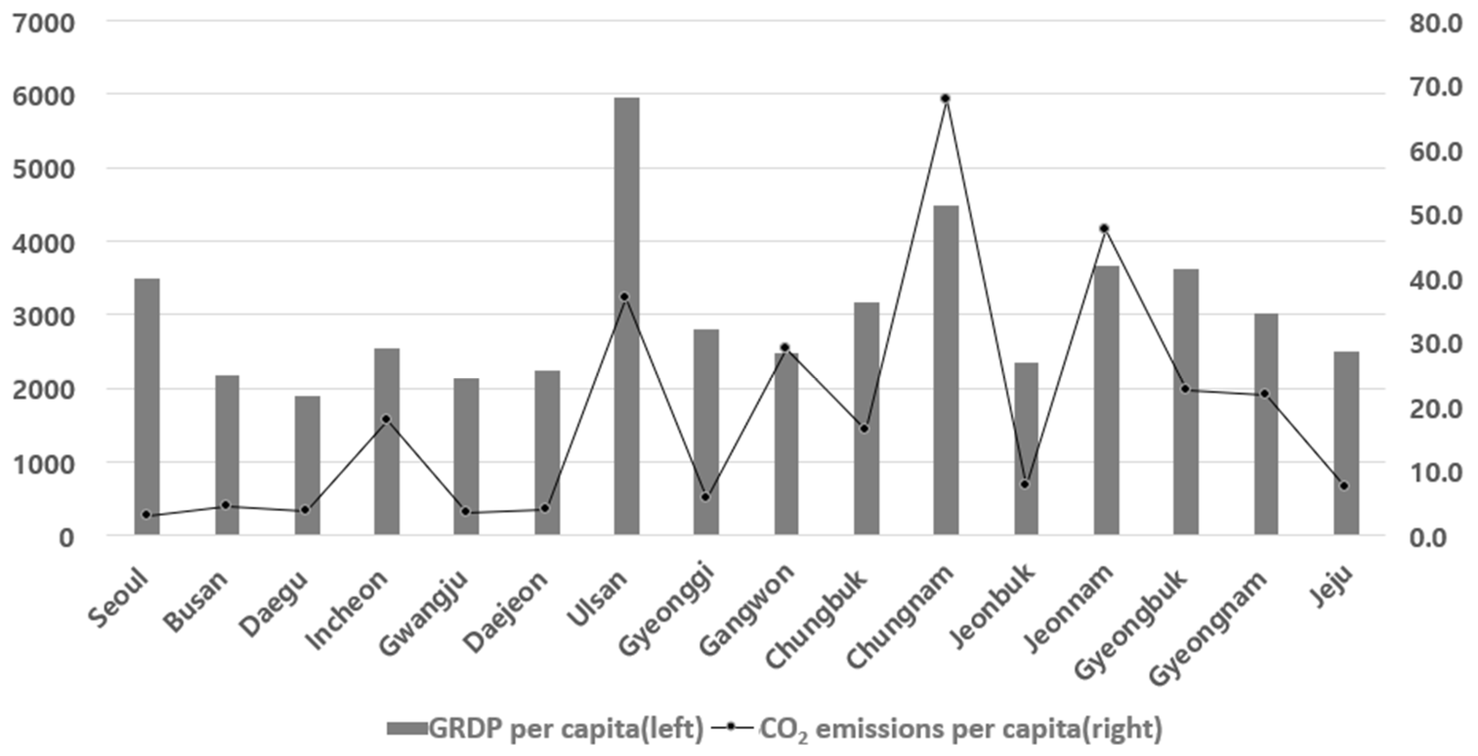
Figure 1. GRDP per capita (in KRW) and CO2 emissions per capita (in tons).
Sustainability 15 14913 g001
Figure 2. The proportions of fiscal expenditure for air quality (%) and per-capita CO2 emissions (tons).
Sustainability 15 14913 g002
Figure 3. Direct, indirect, and total effects.
Sustainability 15 14913 g003
Table 1. Data description.
VariableUnitMeanStd. Dev.MinMax
Gross regional domestic product (GRDP)Ten thousand KRW/person3030.31102.41504.96537.0
Fiscal expenditure for air quality (AEXP)Ten thousand KRW/person404.2497.70.72799.0
CO2 emission (CO2)tons/person18.718.23.074.0
Number of workers (LABOR)1000 people1579.81577.6284.06790.0
Value of tangible assets (CAPITAL)Million KRW/person8712.98207.3382.430,274.2
Final energy consumption per GRDP (ENERGY)1000 toe/person394.3281.834.91161.2
Industrial area (INDUSTRY)1000 m2/1000 people30.523.82.193.9
Energy Price Index (EPI)2020=100116.310.899.5132.6
Sources: Statistics Korea, Ministry of the Interior and Safety, Ministry of Environment, Korea Energy Economics Institute, and Korea Land & Housing Corporation.
Table 2. Estimation Results: First Stage.
Pooled OLSFixed EffectSystem-GMM
l n ( G R D P i t 1 )
 
0.980 ***
(−0.010)
0.661 ***
(−0.041)
0.866 ***
(−0.024)
l n ( A E X P i t )
 
−0.001
(−0.002)
0.008 ***
(−0.002)
0.008 ***
(−0.002)
ln L A B O R i t
 
0.004
(−0.006)
0.133
(−0.084)
−0.011
(−0.008)
l n ( C A P I T A L i t )
 
0.002
(−0.003)
0.098 ***
(−0.027)
0.007
(−0.009)
l n ( E N E R G Y i t )
 
−0.005
(−0.006)
−0.179 ***
(−0.022)
0.020 ***
(−0.007)
Constant
 
0.086 *
(−0.048)
0.441
(−0.501)
0.423 ***
(−0.083)
Hansen test 0.115
AR(1) 0.011
AR(2) 0.172
Notes: Robust standard errors are in parentheses; * and *** denote significance at the 10% and 1% levels, respectively.
Table 3. Estimation Results: Second Stage.
Pooled OLSFixed EffectSystem-GMM
l n ( C O 2 i t 1 )
 
0.986 ***
(−0.015)
0.389 ***
(−0.081)
0.585 ***
(−0.110)
l n ( A E X P i t )
 
−0.004
(−0.005)
−0.012 *
(−0.007)
−0.017 **
(−0.008)
E l n ( G R D P i t )
 
0.352
(−0.473)
−0.039
(−0.641)
6.714 **
(−3.160)
E l n 2 ( G R D P i t )
 
−0.053
(−0.067)
0.043
(−0.088)
−0.912 **
(−0.451)
ln L A B O R i t
 
−0.036
(−0.025)
−0.391 *
(−0.230)
−0.409 ***
(−0.112)
l n ( C A P I T A L i t )
 
0.010
(−0.014)
0.068
(−0.079)
0.005
(−0.055)
l n ( E N E R G Y i t )
 
0.038 *
(−0.021)
0.063
(−0.067)
0.382 ***
(−0.096)
l n ( I N D U S T R Y i t )
 
−0.017
(−0.023)
0.156 *
(−0.092)
0.077
(−0.083)
l n ( E P I i t )
 
−0.148 **
(−0.072)
−0.050
(−0.074)
−0.162 **
(−0.067)
Constant
 
0.153
(−0.819)
2.669
(−1.633)
−10.028 *
(−5.297)
Hansen test 0.143
AR(1) 0.071
AR(2) 0.974
Notes: Robust standard errors are in parenthesis; *, ** and *** denote significance at the 10%, 5% and 1% levels, respectively.
Table 4. Direct, indirect, and total effects by region.
RegionGRDP per CapitaDirect EffectIndirect EffectTotal Effect
Seoul3398−0.0170.002−0.015
Busan2291−0.0170.009−0.008
Daegu2018−0.0170.01−0.007
Incheon2659−0.0170.006−0.011
Gwangju2207−0.0170.009−0.008
Daejeon2277−0.0170.009−0.008
Ulsan5731−0.017−0.006−0.023
Gyeonggi2881−0.0170.005−0.012
Gangwon2571−0.0170.007−0.01
Chungbuk3143−0.0170.004−0.013
Chungnam4444−0.017−0.002−0.019
Jeonbuk2481−0.0170.007−0.01
Jeonnam3768−0.0170.001−0.016
Gyeongbuk3662−0.0170.001−0.016
Gyeongnam3081−0.0170.004−0.013
Jeju2493−0.0170.007−0.01
Disclaimer/Publisher’s Note: The statements, opinions and data contained in all publications are solely those of the individual author(s) and contributor(s) and not of MDPI and/or the editor(s). MDPI and/or the editor(s) disclaim responsibility for any injury to people or property resulting from any ideas, methods, instructions or products referred to in the content.