Collaborative Development and Transportation Volume Regulation Strategy for an Urban Agglomeration

Abstract

Transportation plays an important role in urban development and the formation of urban agglomerations. Indexes including urban centrality, urban development intensity, and degree of urban development imbalance are defined to measure the level of urban development, and are taken as the basis for transportation regulation within urban agglomerations. Regulation of transportation volume is divided into static and dynamic regulation, and this paper studies static regulation. There are two purposes for static regulation. One is to solve the problems of unbalanced urban development and collaborative development, and the other is to solve the problem of rational utilization of the highway transport network in an urban agglomeration so that the total transportation volume of the urban agglomeration does not exceed the total transportation volume that the transport network can bear, realizing coordinated transport, improving transport efficiency, and reducing traffic congestion and traffic accidents. A distributed intelligent regulation model based on the principle of game control is proposed, which is divided into three layers: macro-regulation (government layer), meso-regulation (urban agglomeration layer), and micro-regulation (individual city game layer). The regulation strategies and methods of the urban agglomeration layer and individual city game layer are given, and are verified and illustrated using as the research object called the Jilin Province urban agglomeration in the northeast of China. The paper contributes to the field by presenting innovative research and provides important theories and methods for collaborative development and transportation within urban agglomerations.

1. Introduction

Within a certain geographical scope (urban agglomeration), there is a strong relationship between urban development and transportation, and transportation plays a vital role in urban regional competitiveness and economic development. Transportation guides and promotes the development of regional economic and social activities and the evolution of the spatial structures of regional organizations, while urban development in turn promotes the development of transportation and provides corresponding resource support for transportation [1,2]. Transportation is the main driving force of urban development [3], and is a catalyst for urban development through direct, indirect, and induced effects [4].

Many scholars have studied the relationship between transportation and the development of urban agglomeration from different perspectives. Zhao [5] reported that due to the effect of transportation, cities are more and more closely linked, and urban agglomerations have gradually formed. Melo et al. [6] reported that public transport can effectively enhance the agglomeration effect within cities. Wei et al. [7] concluded that the transportation convenience brought by the integration of land transportation improve the agglomeration of urban agglomeration service industries. Tokunova et al. [8] solved the problem of high-load traffic routes between the St. Petersburg urban agglomeration and the Leningrad region, promoting regional coordinated development. Zou et al. [9] took the comprehensive traffic of Beijing, Tianjin, and Hebei in China as the research object, establishing a traffic-integration model to alleviate the problem of traffic density in the urban central area, and achieving the goal of maximizing regional traffic efficiency. Arbabi et al. [10] put forward an agglomeration strategy dominated by intercity traffic to solve the problem of coordinated development of the regional economy in England. Taking the urban agglomeration of the Guanzhong Plain in China as the research object, Zhao et al. [11] established a comprehensive traffic-carrying-capacity model to analyze the changes in integrated transportation systems. Liu et al. [12] put forward the theory of freight structure and the adaptability-evaluation model of freight supply and demand structure in urban agglomerations. Liu et al. [13] proposed a traffic-supply model based on entropy theory to analyze the equilibrium state of the traffic structure in urban agglomerations, so as to achieve the best economic and social benefits. Hong et al. [14] used sample data from 31 provinces in China to effectively prove that land transport and water transport have an important impact on the economy, while the contribution of transport facilities such as aviation is weak. Yang et al. [15] proved that there is a strong relationship between highway transport and China’s economic growth, while the relationship between railway transport and economic activities is weak.

Based on relevant research works, we can draw the following conclusions: (1) Transportation has an important influence on the formation and development of urban agglomeration; (2) Highway transportation, especially highway freight transportation, has a direct effect on urban development; (3) Most of the existing literature studies the relationship between transportation and other factors of economic development (such as population, urban construction, etc.) and the evaluation and improvement of transportation systems, etc. There is a lack of relevant research works based on the regulation and control of transportation, including the realization of urban collaborative development, rational use of transport networks and collaborative transportation in urban agglomerations, and promoting the high-quality development of urban agglomerations.

We know that the regulation and control of railway and air traffic is very mature, making good use of railway resources and air routes, and promoting the coordinated development of various cities. However, highway transportation has not been regulated and controlled, resulting in many traffic problems. With the development of urban agglomeration and the rapid increase of transport vehicles, if city individuals consider only the maximization of their own interests and ignore coordinated development with the surrounding cities, it will inevitably lead to unbalanced use of transportation-infrastructure resources. As highway transportation capacity is limited, when the transportation distribution between cities is out of balance, it causes traffic congestion, a substantial increase in accidents, and a decrease in transportation efficiency, and indirectly increases carbon emissions, energy consumption, and environmental pollution. From the viewpoint of urban control and management systems, based on the concept of transportation, the superiority of macro-control can be brought into full play by coordinating inter-city transportation volume and realizing the regulation and control of transportation in the urban agglomeration. The purpose is to reduce congestion, reduce accident rates, control carbon emissions and environmental pollution, increase safety and security assurance, optimize travelling speed and traffic flow, and improve transportation efficiency. Therefore, for an urban agglomeration, because the transportation capacity of the transport network is limited, it is necessary, feasible, and of great significance to reasonably distribute or regulate the individual city’s transportation volume and to realize collaborative development and cooperative transportation. This paper studies the regulation and control of highway transportation, which is similar to that of railway and air transportation.

Transportation volume regulation is divided into static and dynamic regulation, and there are two purposes of static regulation. One is to solve the problems of unbalanced urban development and collaborative development, and the other is to solve the problem of rational utilization of the highway transport network in an urban agglomeration. Dynamic regulation will be introduced in a follow-up study. This paper studies static regulation, focusing on individual cities’ collaborative development and collaborative transportation in urban agglomerations, based on transportation. Jilin Province urban agglomeration in the northeast of China is taken as the research object, and the regulation strategies and methods have been verified in the urban agglomeration. The main innovations are as follows: (1) A distributed intelligent regulation model based on the principles of game control and distributed control is proposed, which is divided into three layers: macro-regulation (government layer), meso-regulation (urban agglomeration layer) and micro-regulation (individual city game layer); (2) Regulation strategies of the macro-regulation layer and individual cities’ game strategy in the individual game layer are studied, and a priority regulation strategy for individual cities is innovatively put forward. To solve the multi-objective optimization game, the solution method of a “neighbor game” strategy is indicated according to the characteristics of transportation regulation; (3) It provides an important theoretical method for the intelligent regulation of transportation, the realization of collaborative transportation, and collaborative development among cities in urban agglomerations.

The remainder of this paper is organized as follows. Section 2 introduces the conceptual and mathematical definitions within the study. Section 3 introduces the structural characteristics of the urban agglomeration studied in this paper. Section 4 presents intelligent regulation and control strategies for transportation. Section 5 introduces a case study and simulation. Section 6 provides a summary of the study.

2. Concept and Definition

To discuss the methods used in this study, some of concepts are defined as follows.

2.1. Quantitative Indexes of Urban Development

2.1.1. Urban Centrality

Urban centrality measures the development status and level of a city in an urban agglomeration and reflects the intensity of the individual city’s driving effect on the surrounding area. The indexes of geometric centrality, population centrality, economic centrality, and transportation centrality are used to describe urban centrality, which is the average of the above four indexes.

(1)

Geometric centrality

In order to quantify urban centrality, the concept of physical “center of gravity” is used to define the geometric center point and geometric centrality. If the urban agglomeration area is regarded as a plane, then there exists a point where the sum of distances between the point and other points in the plane must be the minimum, which is called a geometric center point. A geometric center point is calculated as follows:

$$\mathrm{G}\mathrm{C}\mathrm{P}(X_m,Y_m)=\mathrm{m}\mathrm{i}\mathrm{n}(\sum _{m=1}^k\sum _{n=1}^k(\sqrt{{\left(X_m-X_n\right)}^2+{\left(Y_m-Y_n\right)}^2}))$$

(1)

where $\left(X_i,Y_i\right)$ is the latitude and longitude of each point, and K is the number of points in the region. Because the center point is equal to the fulcrum where all the torques are balanced in the region plane, we take the 10 km pixel as the reference cell to griddle the research area and extract the center point of the grid. Urban geometric centrality is calculated as follows:

$${\mathrm{U}}_{gc}=\frac{GDS}{UDS}$$

(2)

$$GDS=\sum _{i=1}^k\sqrt{{\left(X_0-X_i\right)}^2+{\left(Y_0-Y_i\right)}^2}$$

(3)

$$UDS=\sum _{i=1}^k\sqrt{{\left({UX}_0-X_i\right)}^2+{\left({UY}_0-Y_i\right)}^2}$$

(4)

where $\left(X_0,Y_0\right)$ is the geometric center point of the urban agglomeration, $\left(U{X}_0,{UY}_0\right)$ is the geometric center point of a city, $\left(X_i,Y_i\right)$ is the geometric center point of the grid, GDS is the sum of the straight line distances from the geometric center point of the urban agglomeration to each point, and UDS is the sum of the straight line distances from the geometric center point of the city to each point. It is known that the larger ${\mathrm{U}}_{gc}$ is, the closer the city is to the geometric center. Figure 1 shows the geometric center point and the urban geometric centrality.

(2)

Population centrality and economic centrality

Urban development is affected by many factors, and most studies have used population, economy, and other factors to describe urban characteristics and differences. In order to obtain a more objective urban centrality, the population centrality and economic centrality are used to quantify urban centrality. First, the population center point or economic center point of a city is calculated as the follows:

$$\overline{X}=\frac{\sum _{i=1}^k{P}_i{X}_i}{\sum _{i=1}^k{P}_i}, \overline{Y}=\frac{\sum _{i=1}^k{P}_i{Y}_i}{\sum _{i=1}^k{P}_i}$$

(5)

where ($\overline{X}$,$\overline{Y}$) is the population center point or economic center point of a city, ($X_i$,$Y_i)$ is the geometric center point of county-level cities which are included in an urban area, $P_i$ is the county-level city population or city GDP, and K is the number of county-level cities.

According to the torque calculation formula, population centrality or economic centrality of city j is calculated as follows:

$$U_{Pj} or U_{Gj}=\frac{\sum _{i=1}^k{P}_i\times L_{ij}}{\sum _{i=1}^k{P}_i\times D_{ij}}$$

(6)

where $P_i$ is the county-level city population or city GDP, $L_{ij}$ is the straight line distance from each county-level city i to the population or economic center point of the city j,$D_{ij}$ is the straight line distance from each county-level city i to the city j, ${ U}_{Pj}$ is the population centrality, and ${ U}_{Gj}$ is the economic centrality.

(3)

Transportation centrality

Transportation centrality is used to measure the importance and radiation intensity of a city in the transportation network. Referring to the calculation method of geometric centrality, the calculation of transportation centrality is as follows:

$${\mathrm{T}\mathrm{C}}_j=\frac{S_2}{S_1}$$

(7)

$$S_1=\sum _{i=1}^k\sqrt{{\left(X_0-{UX}_i\right)}^2+{\left(Y_0-{UY}_i\right)}^2}$$

(8)

$$S_2=\sum _{i=1}^{k-1}{D}_{ji}$$

(9)

where $\left(X_0,Y_0\right)$ is the geometric center point of the urban agglomeration, $\left(U{X}_i,{UY}_i\right)$ is the geometric center point of a city, $D_{ji}$ is highway transportation mileage from city j to city i, and k is the number of cities.

When urban development changes, the total population, GDP, and the urban centrality change accordingly, and the corresponding grade of a city is upgraded or degraded, which also affects the dynamic change and development of urban agglomerations.

2.1.2. Urban Development Intensity

There are various indexes for the evaluation of urban development [16,17,18]. International authoritative research institutions have put forward indexes such as urban development power and urban competitiveness to describe the current situation of urban areas and compare them with each other. Referring to various index systems, from the aspects of economy, transportation, and urban construction, seven secondary-level indexes such as GDP, urban built-up area, urbanization rate, total population at the end of the year, urban road length, total passenger transportation volume, and freight transportation volume were selected to measure the intensity of urban development. The index of urban development intensity is defined as shown in

Table 1. Evaluation indexes of urban development intensity.

	First-Level Indexes	Second-Level Indexes
Urban development intensity (UI)	Economy (U1)	GDP (U11)
	Urban construction (U2)	Urban built-up area (U21)
		Urbanization rate (U22)
		Population (U23)
	Transportation (U3)	Urban road length (U31)
		Passenger transportation volume (U32)
		Freight transportation volume (U33)

. Urban development intensity can reflect the comprehensive competitiveness of urban development.

After principal component analysis, two principal components (F1 and F2) were extracted. The eigenvalues are 5.916 and 1.001, respectively, and the cumulative contribution rate of variance is 98.824%. So, the two new variables can be used to replace the original seven variables. Due to the standardized processing of the data, some weights are negative.

UI = 0.84517 × F1 + 0.14307 × F2

(10)

F1 = 0.068 × U11 + 0.069 × U21 − 0.018 × U22 + 0.070 × U23 + 0.068 × U31 +
0.069 × U32 + 0.071 × U33

(11)

F2 = 0.024 × U11 + 0.027 × U21 + 0.992 × U22 − 0.020 × U23 + 0.037 × U31 −
0.028 × U32 − 0.084 × U33

(12)

2.2. Transportation

In an urban agglomeration that relies on railways, highways, and other roads, there are a large number of dense and multi-category transport networks among cities, and city individuals are closely connected by various modes of transport. According to statistics, the freight volume of land transport in most countries accounts for more than 70% of the total transport volume [19].

Transportation volume is divided into passenger and freight transportation volume. The benefits brought by freight transportation directly affect a city’s economic development. Most scholars regard freight transportation volume as an important index of urban classification in the study of urban agglomeration. Therefore, this study mainly focuses on freight transportation volume. The freight transportation volume for a single day (or month, year) is calculated, and its unit is tons. For highway transportation, if the highway freight transportation volume is given, it can be converted into the number of standard vehicles according to the average carrying weight of the transportation vehicles.

Highway transportation is also divided into expressway transportation and other highway transportation networks (including national, provincial, county, and township roads). The transportation volume of expressways is relatively large in the transportation relationship between urban areas, which is a key object of research and regulation. Expressway transportation is mainly highway transportation, and the transportation generated by other non-expressway networks serves as a supplement to expressway transportation.

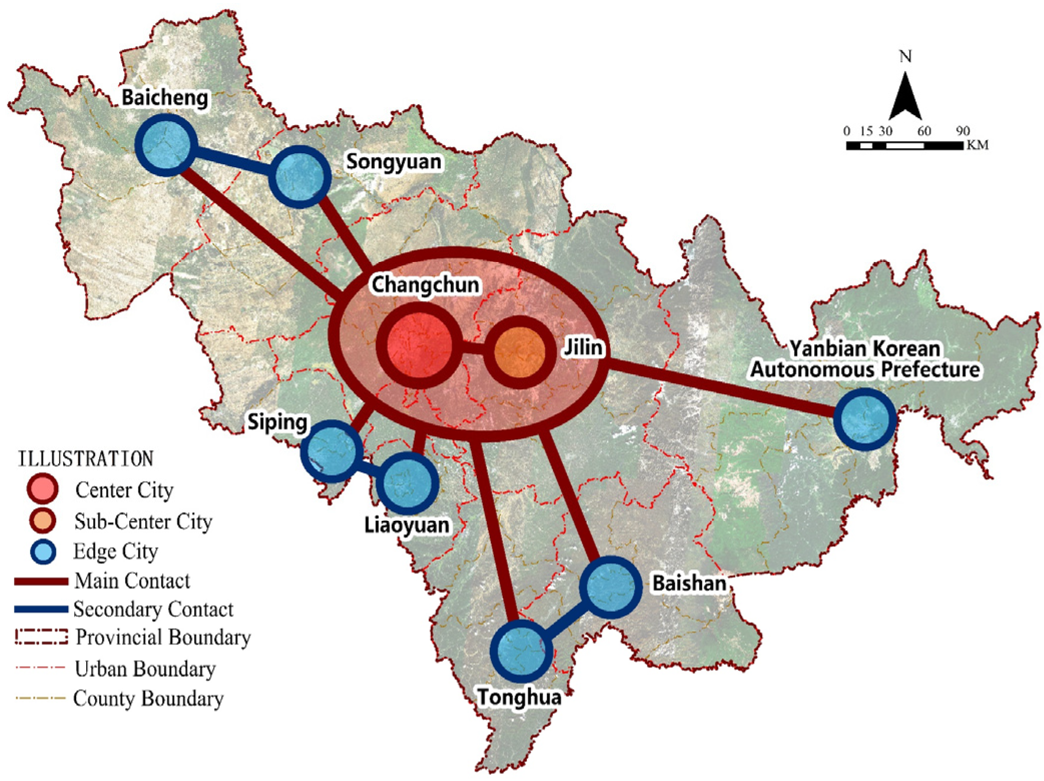
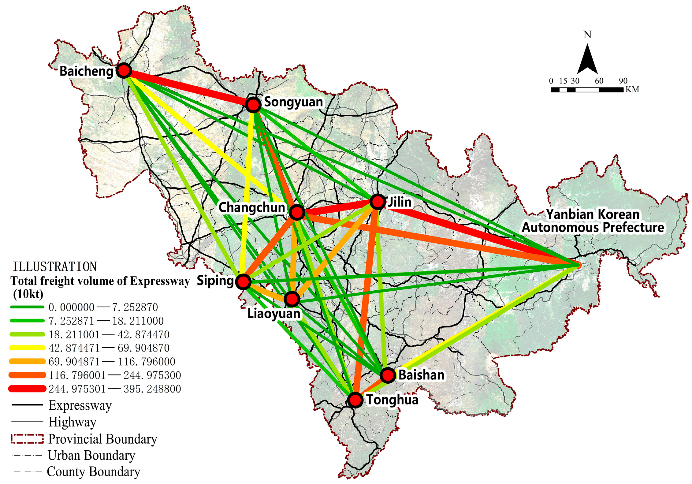
3. Research Object and Data

3.1. Indexes Calculation

Jilin Province is located in the northeast of China, and the research object is the urban agglomeration in Jilin Province, including the nine major cities of Changchun (CC), Jilin (JL), Baicheng (BC), Songyuan (SY), Siping (SP), Liaoyuan (LY), Tonghua (TH), Baishan (BS), and Yanbian Korean Autonomous Prefecture (YB).

Table 2. Values of indexes for each city.

City	Geometric Centrality	Population Centrality	Economic Centrality	Transportation Centrality	Urban Centrality	Grade of City
Changchun	0.949	0.997	0.906	0.856	0.927	Central city
Jilin	0.981	0.875	0.760	0.717	0.833	Sub-central city
Baicheng	0.535	0.423	0.347	0.421	0.431	Marginal city
Songyuan	0.749	0.338	0.558	0.585	0.557	Marginal city
Siping	0.795	0.744	0.671	0.753	0.740	General city
Liaoyuan	0.857	0.787	0.704	0.759	0.776	General city
Tonghua	0.695	0.524	0.433	0.624	0.569	Marginal city
Baishan	0.751	0.555	0.456	0.601	0.590	Marginal city
Yanbian	0.627	0.397	0.308	0.407	0.434	Marginal city

shows the geometric centrality, population centrality, economic centrality, transportation centrality, and urban centrality calculated for each urban area. Urban centrality is the average of geometric centrality, population centrality, economic centrality, and transportation centrality, which comprehensively reflects the geographical location, population, economy, and transportation network of a city. According to the characteristics of average centrality, cities are divided into four levels: central city, sub-central city, general city, and marginal city.

The calculation results show that the urban agglomeration takes Changchun–Jilin as its development center, and the development of other urban areas is weak. Figure 2 shows the distribution of geometric centers, population centers, and economic centers of the urban agglomeration and the relationships between major cities and various centers. We can see from Figure 2 that all kinds of centers are distributed near the two major cities of Changchun and Jilin. It shows that Changchun and Jilin are the central areas of the urban agglomeration, Changchun is the central city, and Jilin is the sub-central city. Other cities are general cities or marginal cities. The urban development is out of balance, and the overall development of the urban agglomeration is not good, and needs to be regulated to support the high-quality coordinated development of urban agglomeration.

Table 3. Values of development intensity for each city.

City	GDP (RMB Ten Thousand)	Built-Up Area (km2)	Urbanization Rate (%)	Population (Ten Thousand)	Road Length (km)	Passenger Transportation (Ten Thousand)	Freight Transportation (Ten Thousand Tons)	Development Intensity
CC	71,031,157	654.19	66.83	908.72	4645.43	2882	20,550	0.882
JL	15,499,802	267.2	64.12	354.73	2569.57	1681	4909	0.187
YB	5,540,239	89.06	51.99	176.98	547.71	732	7811	0.039
BS	4,634,867	50.23	58.32	97.91	192.3	468	1538	–0.011
TH	5,679,048	74.07	61.3	177.12	316.62	666	1645	–0.171
SP	5,414,054	49.58	79.64	98.39	369.89	484	996	–0.223
SY	8,177,054	70.78	47.68	219.48	432.3	1027	6847	–0.249
LY	5,488,325	92.06	54.97	150.76	613.09	271	986	–0.252
BC	8,011,692	163.85	76.94	191.28	968.95	944	2392	–0.257

shows the specific values of the indexes and the calculation results of urban development intensity. In the current urban agglomeration, Changchun has a strong development intensity, followed by Jilin, and other cities have weak development intensity. Due to the standardized processing of the data, some values are negative.

The difference between urban centrality and urban development intensity is defined as the imbalance degree of urban development, as shown in

Table 4. Values of imbalance degree.

City	Urban Centrality	Urban Development Intensity	Imbalance Degree
CC	0.927	0.882	0.045
JL	0.833	0.187	0.696
BC	0.431	–0.257	0.688
SY	0.557	–0.249	0.806
SP	0.740	–0.223	0.963
LY	0.776	–0.252	1.028
TH	0.569	–0.171	0.740
BS	0.590	–0.011	0.601
YB	0.434	0.039	0.395

. The imbalance degree is large, which shows that although the city has good urban centrality, its urban development is not good. The imbalance degree is small, which means that the urban development is good.

As shown in Table 4 and Figure 3, the development of the urban agglomeration is mainly concentrated in the central region with Changchun as the center and Jilin as the sub-center. The population center, economic center, and transportation center are all located near the junction of Changchun and Jilin (also see Figure 2). The urban areas with high correlation degrees of population, economy, and transportation are concentrated in the middle and south of the urban agglomeration. The correlation degrees of other urban areas are low, the difference of the centrality value is obvious, and the regional connection is weak. This indirectly leads to the slow development of other urban areas in the urban agglomeration, especially in the remote marginal urban areas which develop particularly slowly. The imbalanced and uncoordinated development can be improved by regulating the transportation volume among the cities.

3.2. Relationship between Transportation and Urban Development (GDP)

Figure 4 shows the distribution of transportation volume among cities in the urban agglomeration. Obviously, the most developed highway traffic is the central part of Jilin Province, which is dominated by Changchun–Jilin–Siping–Liaoyuan. The freight volume of Baicheng–Songyuan–Changchun–Jilin–Yanbian, Jilin–Tonghua, Tonghua–Baishan, and Changchun–Siping is relatively large, and the corresponding expressways are G12, G1112, G11, and G1.

GDP (unit: RMB 100 million) is the sum of the GDP of primary industry, secondary industry, and tertiary industry. The GDP values of the primary, secondary, and tertiary industries in Jilin Province account for 12.92%, 35.41%, and 51.67%, respectively. With the development of social economy, the proportion of GDP resulting from tertiary industry is increasing. Transportation belongs to tertiary industry and has an important impact on GDP growth.

Quarterly gross domestic product (GDP) and expressway transportation volume data were obtained from the Statistical Yearbooks from 2018 to 2022. After estimation using a variety of regression curves, the correlation between highway transportation volume and GDP for each city is as follows:

$$\mathrm{Jilin}: {GDP}_{jl}=445.9289-1.2332x+0.0028x^2$$

(13)

$$\mathrm{Changchun}: {GDP}_{cc}=1582.1534-0.5258x+0.00041x^2$$

(14)

$$\mathrm{Songyuan}: {GDP}_{sy}=349.1899-1.2584x+0.0026x^2$$

(15)

$$\mathrm{Siping}: {GDP}_{sp}=118.4132-0.0884x+0.00098x^2$$

(16)

$$\mathrm{Liaoyuan}: {GDP}_{ly}=259.8054-3.6761x+0.0203x^2$$

(17)

$$\mathrm{Tonghua}: {GDP}_{th}=160.0286-1.1111x+0.0053x^2$$

(18)

$$\mathrm{Baishan}: {GDP}_{bs}=146.0471-1.7693x+0.0155x^2$$

(19)

$$\mathrm{Baicheng}: {GDP}_{bc}=134.9378-0.7536x+0.0041x^2$$

(20)

$$\mathrm{Yanban}: {GDP}_{yb}=180.0044-0.3706x+0.0014x^2$$

(21)

where GDP is the quarterly gross domestic product, unit: RMB 100 million, x is quarterly expressway transportation volume, unit: ten thousand vehicles.

$$\mathrm{GDP} \mathrm{increment}: ∆GDP={GDP}^{\prime }\times ∆ x$$

(22)

By calculating the derivatives of Equations (13)–(21) and making them zero, the minimum transportation volume that makes the GDP increment greater than zero can be obtained, as shown in

Table 5. Minimum transportation volume.

City	JL	CC	SY	SP	LY	TH	BS	BC	YB
Quarterly minimum volume	220	641	242	45	90	104	57	91	132
Annual average minimum	880	2564	968	180	320	416	228	364	528
Daily average minimum	2.4444	7.1222	2.6888	0.500	1.0000	1.1555	0.6333	1.0111	1.4666

.

The urban quarterly average GDP growth rate in the current year is set as X %, and last year’s quarterly average GDP as Y; then, the quarterly GDP increment for the current year is:

$$∆GDP=\frac{X\times Y}{100}$$

(23)

Using Equation (22), $∆x$ can be calculated. The quarterly average minimum transportation volume that guarantees quarterly GDP growth in the current year is:

$$x_{min}=x_p+∆ x$$

(24)

where $x_p$ is the quarterly average transportation volume last year.

The calculated minimum transportation volume provides an important reference for the transportation regulation of the urban agglomeration and the realization of collaborative development among cities. It shows that each city has a minimum transportation requirement to ensure its normal development.

4. Intelligent Regulation and Control Strategy for Transportation

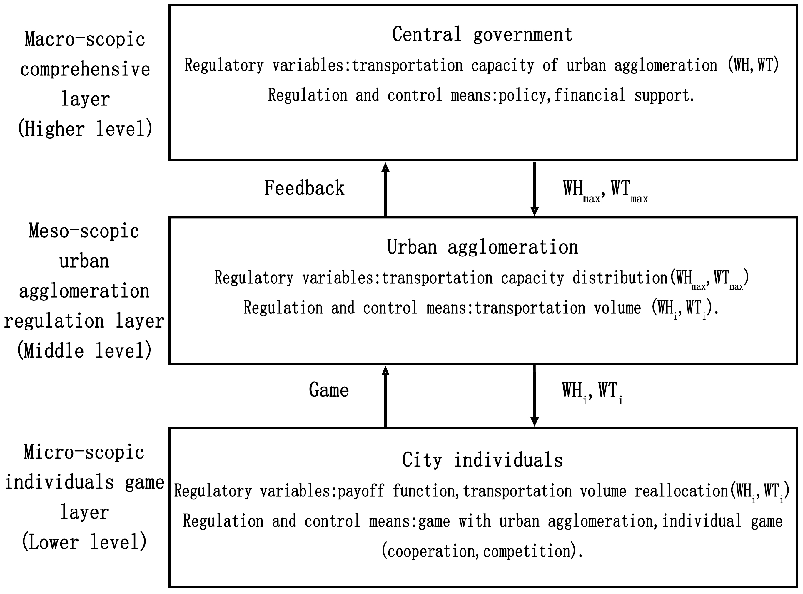
4.1. Distributed Intelligent Regulation Principle

Based on the above analysis, the following conclusions are drawn: (1) The development of each city in the urban agglomeration is unbalanced, and the urban agglomeration needs collaborative development; (2) Transportation plays an important role in urban development and directly affects the GDP value of tertiary industry; (3) The transportation network in the urban agglomeration has a given maximum transportation capacity. If it is not regulated and controlled, each city will seize the transport network in order to pursue its own best interests, which will inevitably lead to road congestion and low transportation efficiency. At the same time, this situation aggravates the imbalance of development between urban areas; (4) Because of the important role of transportation in urban development, collaborative development can be realized by regulating the distribution of transportation volume among cities in the urban agglomeration. On the other hand, this can also improve transportation efficiency. Therefore, it is necessary to study the strategies and methods of transportation regulation and control in urban agglomerations. No matter whether between each individual city and the urban agglomeration, or between individual cities, the regulation and control process of transportation volume is a process of interest redistribution, and the process of interest distribution is a game process. The participants want to pursue benefit maximization, so this requires a regulator to uniformly regulate the interests of all participants. The principle and method of game control are very suitable for solving the above problem of transportation volume allocation. We propose a distributed intelligent regulation system based on the principle of game control.

Game control is a cross-disciplinary combination of game theory and control theory, that has emerged in recent years [20,21,22,23,24,25,26,27,28]. It is characterized by a hierarchical regulatory framework that includes the upper and lower layers. The upper layer consists of macro-control variables, and the lower layer consists of multiple individuals with interrelated and different functions. The purpose of macro-control is that the overall function of the system achieves the desired goal, while ensuring the basic rights and interests of the individuals. If the non-cooperative game among the lower individuals forms a poor Nash equilibrium, then game-based control is used for the regulation and control of the Nash equilibrium. If the game among the individuals loses a good dynamic balance, then game-based regulation is expected to restore and maintain the balance through dialectical treatment. At the same time, the man–machine fusion system can affect group consensus and group action.

A distributed control system is a typical control architecture of a computer control system [29] and is generally divided into three layers. The lower layer is the control layer, the middle layer is the regulation and control layer, and the upper layer is the integrated information management layer. The three layers are linked together by a specific network architecture that has the functions of distributed control and centralized management to ensure the best control performance of the entire system.

With the combination of distributed control ideas and the principle of game control, and according to the characteristics of urban agglomeration transportation regulation, we propose an intelligent regulation and control framework for urban agglomeration transportation. It is called a distributed intelligent regulation system, based on game–control theory, as shown in Figure 5. The three-layer regulation structure shown in Figure 5 can effectively solve the problem of transportation volume regulation. Individual city development must be integrated with the development of urban agglomeration, and the overall development of urban agglomeration needs strong support from the government. Under the premise of maximizing individual income, the individual game layer continues the income regulation by the urban agglomeration regulation layer to obtain the best Nashi balanced income. Urban agglomeration reaches a certain level of development, restricted by the bottleneck of transportation volume, sending demands to the government, and obtaining policy and financial support from the government. New highways or railways may be built to accelerate the development of urban agglomeration.

Where WH is the highway transportation volume and WT is the railway transportation volume. As we know, the regulation and control technology for railway transportation is relatively mature; without considering the railway transportation regulation and control, we study only highway transportation regulation and control. As discussed, highway transportation regulation and control has not been realized up to now.

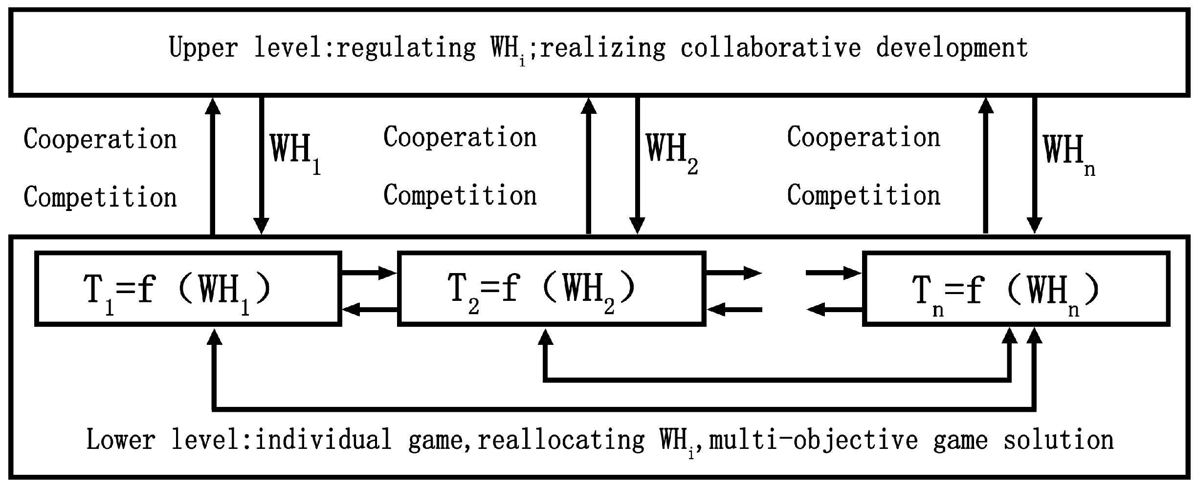
4.2. Game Control Modeling of Transportation Volume Regulation

Assuming that $x_i$ represents the transportation volume for city i and $x_{\min \left(i\right)}$ represents the minimum transportation volume i = 1, 2, … n, the maximum transportation volume of the urban agglomeration transport network is ${\mathrm{W}\mathrm{H}}_{max}$, and the current total transportation volume of the urban agglomeration is WH. Having set X = {$x_1,x_2,\dots x_n$}, the following objective functions for optimization of the individual city can be established. The objective function is the maximum, that is, the individual city pursues the maximum transportation volume.

$$\max f_1\left(x_1\right)=x_1-x_{\min \left(1\right)}$$

(25)

$$\max f_2\left(x_2\right)=x_2-x_{\min \left(2\right)}$$

(26)

$$\max f_n\left(x_n\right)=x_n-x_{\min \left(n\right)}$$

(27)

The objective function for optimization of the urban agglomeration is as follows. The objective function is minimized, that is, the sum of individual cities’ transportation volume does not exceed the maximum transportation volume of the transportation network. Theoretically, the optimal solution is that the objective function value should be 0.

$$\min f\left(X\right)=\sum _{i=1}^n{x}_i-{\mathrm{W}\mathrm{H}}_{max}$$

(28)

St.

$$\sum _{i=1}^n{x}_i\le WH$$

(29)

$$\sum _{i=1}^n{x}_i\le {\mathrm{W}\mathrm{H}}_{max}$$

(30)

$$x_i\ge x_{\min \left(i\right)} \mathrm{or} f\left(x_i\right)\ge 0$$

(31)

Based on the above objective functions, the following conclusions can be drawn. (1) There are contradictions among individual cities, all of which want to pursue the maximum transportation volume, occupy most of the transport network resources, and obtain the maximum income. However, under the given constraints and the given network transport capacity, this is impossible. It is necessary to achieve a reasonable distribution of transportation volume among individual cities through certain game-regulation strategies; this is called Nash equilibrium. (2) There is a contradiction between the individual city and the urban agglomeration as a whole. The objective function of the urban agglomeration seeks the minimum optimal solution, which conflicts with the maximum optimal solution of the individual city’s objective function. From the viewpoint of urban agglomeration regulation and control, the schematic diagram of the feedback control shown in Figure 6 can be used to explain the control principle. The set value in the figure is the maximum transportation volume of the transport network, the controlled variable is the total transportation volume of the urban agglomeration, and the disturbances come from the increase of transportation volume and all kinds of transport vehicles brought about by individual city development. Urban agglomeration should solve the contradiction between individual cities and the urban agglomeration as a whole through certain game-regulation strategies, that is, solving the coordination of overall optimization and local optimization, and ensuring that the total transportation volume of the urban agglomeration does not exceed the maximum transportation volume of the transport network.

For the game control model of transportation volume regulation, the macro-control variable is the current total transportation volume of the urban agglomeration (WH), and the multiple individuals with interrelated and different functions are individual cities.

The individual cities’ game can be expressed as the following non-cooperative game model:

Participants: i = 1, 2, 3, ……………n, n of city individuals.

Strategy group: $x=\left[x_1,x_2,\dots \dots \dots x_n\right],x_i\in R^{m_i}$.

Strategy sets: $X=X_1\times X_2\times \dots \dots \dots X_n,X_i\in R^{m_i}$.

Payoff function: $f_1\left(x\right),f_2\left(x\right),\dots \dots \dots f_n\left(x\right)$.

In this game, the participant i always maximizes its own income, so the corresponding game problem is:

$$\left\{\underset{x_i\in X_i}{\max }{f}_i(x_i, x_{-i})\right\}·········\forall \mathrm{i}$$

(32)

where $x_i$ represents the decision variables for participant i, $x_{-i}$ represents the other decision variables in addition to $x_i$, and $m_i$ represents the number of decision variables for participant i.

$${\sum }_{i=1}^n{m}_i=m \mathrm{m}\ge \mathrm{n}$$

$$x_{-i}=\left[x_1, x_2,\dots ,x_{i-1}, x_{i+1}\dots \dots x_n\right]$$

If strategy $x^{*}$ exists and satisfies the following condition, $x^{*}$ represents Nash equilibrium for the game problem (32).

$$f_i(x_i^{*},x_{-i}^{*})\ge f_i(x_i,x_{-i}^{*})······\forall x_i\in X_i····\forall i$$

(33)

Because there are constraints (29)–(31), it is difficult to find the Nash equilibrium solution for the problem of regulation of urban agglomeration transportation. We propose a priority regulation strategy at the upper layer (urban agglomeration regulation layer) and a “neighbor game” strategy at the lower layer (individual game layer) to find the game-based Pareto optimal solution. These strategies are described in detail later in this paper.

4.3. Distributed Intelligent Regulation Strategies and Methods

The government (higher level) plays a macro-regulative and comprehensive managerial role, and its decision making and policy support are complex. Because it is affected by various factors, the urban agglomeration regulation layer in Figure 5 can only provide feedback demand for transportation capacity to the government, and a demand plan is put forward to the government. Therefore, the urban agglomeration cannot affect the government’s decision making, so we do not consider its functions.

Assuming that ${WH}_i$ represents the highway transportation volume for city i and the urban agglomeration is composed of many city individuals (n). The total highway transportation volume is:

$$WH={\sum }_{i=1}^n{WH}_i$$

(34)

4.3.1. Strategy of Urban Agglomeration Regulation Layer

As discussed above, the urban agglomeration should solve the contradiction between individual cities and the urban agglomeration as a whole through certain game-regulation strategies. The basic regulation strategy is as follows. Assuming that the maximum transportation volume of the urban agglomeration highway transportation network is ${WH}_{max}$, and the sum of transportation volume of each city is WH, there are two cases. First, the total transportation capacity of the urban agglomeration is less than the maximum transportation capacity of the transportation network, that is, $WH<{WH}_{max}$. The transportation network has surplus transportation capacity, and the surplus transportation capacity is calculated:$∆{WH}_L={WH}_{max}-WH$. In this case, we should allocate the surplus capacity to the slowly developing individual cities as far as possible, to speed up their development. Second, the total transportation volume of the urban agglomeration is larger than the maximum transportation volume of the transport network, that is, $WH>{WH}_{max}$. It exceeds the maximum transportation volume of the transport network, and the excess volume is: $∆{WH}_S=WH-{WH}_{max}$. We should reasonably regulate the individual cities’ transportation volume, in other words, reduce the transportation volume so the total transportation volume of the urban agglomeration does not exceed the maximum transportation volume of the transportation network.

(1)

Surplus transportation capacity allocation

This can be allocated according to the proportion of imbalance degree of each city, as shown in Table 4. If the proportion of the individual city’s imbalance degree is $\mathrm{N}{B}_i$, the increase of transportation volume for individual city i can be calculated:

$$∆{WH}_i=∆{WH}_L\times {NB}_i$$

(35)

where ${NB}_i=\frac{{UNB}_i}{\sum _{i=1}^n{UNB}_i}$, ${U\mathrm{N}\mathrm{B}}_i$ is the imbalance degree of city i.

The proportion of imbalance degree is large, corresponding to the slow development of a city. The amount of allocated transportation volume is also large, and satisfies the requirements of collaborative development.

(2)

Excess transportation capacity regulation

For the second case, the individual city’s transportation volume should be reduced, and the regulated transportation volume ${{WH}_i}^{*}$ should satisfy the following condition:

$${\sum }_{i=1}^n{{WH}_i}^{*}\le {WH}_{max}$$

(36)

and ${{WH}_i}^{\mathrm{*}}\ge {WHmin}_i$ where ${WHmin}_i$ is the minimum transportation volume of a city. According to the requirements of collaborative development, we adopt the basic regulation rules of “ensuring the ends, regulating the middle, helping the cities with slow development speed, and realizing collaborative development”. Priority strategies for regulation and control are put forward.

The meaning of “ensuring the ends and regulating the middle” is as follows. The individual cities are sorted from small to large according to urban centrality; the largest is generally the central city and the smallest is the marginal city. The city with the largest centrality plays a leading role in an urban agglomeration, and it has priority to ensure the completion of its transportation tasks and its development. The city with the smallest centrality develops slowly, and its transportation volume should not be regulated, in order to ensure its rapid development driven by the urban agglomeration. Therefore, only the remaining individual cities (n-2) in the middle regulate their transportation volume.

The meaning of “helping the cities with slow development speed and realizing collaborative development” is as follows. The smaller the urban centrality is, the higher the priority of regulation is, and the smaller the reduced transportation volume is. In other words, the city develops relatively slowly, the reduced transportation volume is relatively small, and the actual transportation volume is relatively larger.

In order to ensure the “fairness” of regulation and the diversification of regulation strategies, and to meet the needs of different situations, the following priority regulation strategies are proposed for the remaining individual cities (n-2) in the middle.

(a)

Fixed priority. According to the order of urban centrality from small to large, the regulation priority is fixed from high to low, and each regulation is carried out sequentially according to the priority, which will never change.

(b)

Cyclic priority. The smaller the urban centrality is, the higher the regulation priority is, such that the city with the smallest urban centrality is regulated first. After it is regulated, its priority becomes the lowest and it ranks automatically at the bottom, and the city with the second highest priority then has the highest priority. The regulation is then conducted in accordance with the new priority order, and therefore, the highest priority takes turn.

(c)

Specified priority. According to the comprehensive consideration of urban centrality and urban development, the urban agglomeration layer sets the regulation priority for each city.

Among the above three priority strategies, the cycle priority strategy is relatively fair. The regulatory priorities and weights based on the first priority strategy are listed in

Table 6. Regulation priority case (1).

Urban Centrality from Small to Large	City 1	City 2	City i	City n-2
Regulation priority from high to low	The highest	higher	high	the lowest
Regulation weight from small to large	$K_1$	$K_2$	$K_i$	$K_{n-2}$
Regulated volume	$∆{WH}_1$	$∆{WH}_2$	$∆{WH}_i$	$∆{WH}_{n-2}$

. The next regulation priority is shown in

Table 7. Regulation priority case (2).

Urban Centrality from Small to Large	City 2	City 3	City i-1	City 1
Regulation priority from high to low	The highest	higher	high	the lowest
Regulation weight from small to large	$K_1$	$K_2$	$K_i$	$K_{n-2}$
Regulated volume	$∆{WH}_2$	$∆{WH}_3$	$∆{WH}_{i-1}$	$∆{WH}_1$

where $\sum _{i=1}^{n-2}{K}_i=1$, $K_1<K_2<\dots <K_{n-2}$, $∆{WH}_i=K_i\times ∆{\mathrm{W}\mathrm{H}}_S$.

, according to the cyclical priority strategy.

$∆{WH}_i$ is the transportation volume that city i should be reduced, $∆{\mathrm{W}\mathrm{H}}_S$ is the excess transportation volume; then, the actual transportation volume can be calculated:

$${{WH}_i}^{*}={WH}_i-∆{WH}_i$$

(37)

If ${{WH}_i}^{*}<{WHmin}_i$, then ${{WH}_i}^{*}={WHmin}_i$, that is, the minimum transportation volume should be maintained. The reduced transportation volume is expressed as follows:

$$∆W_i={WH}_i-{WHmin}_i$$

(38)

The remaining reduced transportation volume is as follows:

$$∆{RW}_i=∆{WH}_i-∆W_i$$

(39)

$∆{RW}_i$ can be deducted from the transportation volume ${WH}_{n-2}$, which belongs to the city with the largest urban centrality. If there are k cities whose transportation volume equals to its own the minimum transportation volume, the total remaining reduced transportation volume is:

$$\mathrm{T}\mathrm{R}\mathrm{W}=\sum _{i=1}^k∆{RW}_i$$

(40)

According to the regulation priority strategies, $\mathrm{T}\mathrm{R}\mathrm{W}$ can be deducted from the other urban areas (n-2-k).

The following methods can be used for determining $K_i$, assuming that m = n-2, representing the number of the remaining city individuals.

(a)

Regulation based on the proportional method.

If m = 2, $K_1$ = 0.4, $K_2$ = 0.6;

If m = 3, $K_1$ = 0.2, $K_2$ = 0.3,$K_3$ = 0.5;

If m = 4, $K_1$ = 0.1, $K_2$ = 0.2, $K_3$ = 0.3,$K_4$ = 0.4;

If m ≥ 5, the average division method is used. The city with the largest centrality accounts for half of the total, the second accounts for half of the remaining, and so on. Each of the last two cases accounts for half of the remaining cases. For example, if m = 5, the proportional distribution: $\frac{1}{16}, \frac{1}{ 16},\frac{1}{8}, \frac{1}{ 4}, \frac{1}{2}$.

(b)

Regulation based on the imbalanced degree of urban development

If the proportion of urban imbalance degree is $\mathrm{N}{B}_i$, sorting $\mathrm{N}{B}_i$ from small to large to obtain $\mathrm{N}{B}_j$, then $K_i=$ $\mathrm{N}{\mathrm{B}}_{\mathrm{j}}$. That is, the city with the highest priority has the smallest proportion of regulation, while the one with the lowest priority has the largest proportion of regulation.

4.3.2. Strategy of Individual City Game Layer

As discussed above, there are contradictions among individual cities, and the contradictions should be solved in the individual city game layer. The regulation strategies of the individual city game layer are suitable for the regulation and control of exceeding transportation capacity. Individual cities first play games with the urban agglomeration, choose cooperation strategies, and receive unified regulation and control. After the regulation of the urban agglomeration regulation layer, the individual city obtains the proper transportation volume. The regulated transportation volume returns to the individual game layer, and a city further negotiates within the other individuals to determine the final respective transportation volumes. Because it is a multi-individual game, it is relatively complex. According to the characteristics of the highway transportation network, we use the “neighbor game” strategy.

(1)

Strategy of the “neighbor game”

An individual city chooses two individual cities that are connected with itself to form a tripartite game. The tripartite game reallocates the reduced transportation volume returned from the urban agglomeration regulation layer ($∆{WH}_{\mathit{i}}$). If three individuals select a competitive strategy, there is no need to reallocate the transportation volume, and the regulated transportation volume maintains its original value. If any one of them is willing to select a cooperative strategy, it can negotiate with the partners to reduce its own transportation volume and increase that of the partners. The strategy of the “neighbor game” meets the actual situation of transportation regulation, because only the neighboring individual cities have a great impact on the transportation capacity, and the two individuals who are far away from each other have little influence on the allocation of transport resources. There is a proverb often used in life: “the far relatives are not as good as the close neighbors”.

(2)

Selecting method

The individual city with the largest urban centrality prioritizes the selection of cooperative individual cities. If an individual city is chosen to cooperate with a game group, it will no longer participate in the game of another group. After the selection is completed, the remaining two city individuals form a game group, and the existing mature two-party game strategy can be adopted. If only one individual city remains, there is no cooperation. Because the urban centrality is dynamic, the cooperation is also dynamic, and the formation of cooperative groups is not fixed.

(3)

Regulation goal and method

The regulation goal is to reallocate the reduced transportation volume returned from the urban agglomeration regulation layer ($∆{WH}_{\mathit{i}}$) among the three individuals. Assuming that H represents the total reduced transportation volume, we have:

$$H={\sum }_{i=1}^3∆{WH}_i$$

(41)

The Shapley value method is used to solve the problem. The Shapley value method was put forward by Shapley L.S [30]; it belongs to cooperation game theory and solves the problem of conflict due to the distribution of interests in the process of cooperation. One of the advantages of the Shapley value is that it distributes the benefits according to the marginal contribution rate of the member to the alliance, that is, the benefit shared by the member i is equal to the average value of the marginal interest created by the member for the alliance in which he participates. The benefit distribution of alliance members based on the Shapley value reflects the contribution of alliance members to the overall goal of the alliance, and it avoids equalitarianism in distribution. It is more reasonable and fair, and it also reflects the process of the game among alliance members. The specific calculation is as follows.

When member i participates in the S alliance, there are (|S| − 1)! combinations. |S| represents the number of members contained in the alliance. The combination of the remaining members is (n − |S|)!. The different ranking combinations that all members i participate in divided by the random ranking combination of n members is the weight of the benefits that member i should share in the alliance as a whole, marked as [(|S| − 1)! * (n − |S|)!]/(n!). Member i participates in different alliances S, and the marginal contribution created by member i participating in the alliance is recorded as [v(S) − v(S\{i})]. The benefit of member i from the overall benefit v (N) is as follows:

$${\phi }_i\left(v\right)=\sum _{s\in S_i}\frac{\left(\left|s\right|-1\right)!\times \left(n-\left|s\right|\right)!}{n!}\times \left[v\left(s\right)-v(s\backslash \{i\left\}\right)\right]$$

(42)

The Shapley value method is used to solve the cooperative game problem of the tripartite game (A, B, C), and the urban development intensity (UI) is used to represent each individual city’s income. The value is ranked from large to small, that is, the urban development intensity of A is the largest, followed by that of B, and that of C is the smallest. The cooperation between individuals must promote the development of individual cities. The tripartite cooperation strategies are: A and B cooperation, A and C cooperation, B and C cooperation, and A, B, and C cooperation. The benefits of cooperation to the individual must be greater than those brought about by the individual’s own development.

Table 8. Income of the tripartite game.

Individual Alliance	A	B	C	A + B	A + C	B + C	A + B + C
Income	UI(A)	UI(B)	UI(C)	UI(AB)	UI(AC)	UI(BC)	UI(ABC)
Simulating data	60	40	20	120	140	100	240

shows the income for individuals and cooperations (simulated data).

According to (42), the distribution of benefits of tripartite cooperation are:

$$\begin{gathered} \mathsf{\phi }\left(\mathrm{A}\right)=\frac{UI\left(A\right)}{3\times 1}+\frac{\left(UI\left(AB\right)-UI\left(B\right)\right)+(UI\left(AC\right)-UI\left(C\right))}{3\times 2} \\ +\frac{UI\left(ABC\right)-UI\left(BC\right)}{3\times 1} \end{gathered}$$

(43)

$$\mathsf{\phi }\left(\mathrm{B}\right)=\frac{UI\left(B\right)}{3\times 1}+\frac{\left(UI\left(AB\right)-CI\left(A\right)\right)+(UI\left(BC\right)-UI\left(C\right))}{3\times 2}+\frac{UI\left(ABC\right)-UI\left(AC\right)}{3\times 1}$$

(44)

$$\mathsf{\phi }\left(\mathrm{C}\right)=\frac{UI\left(C\right)}{3\times 1}+\frac{\left(UI\left(BC\right)-UI\left(B\right)\right)+(UI\left(AC\right)-UI\left(A\right))}{3\times 2}+\frac{UI\left(ABC\right)-UI\left(AB\right)}{3\times 1}$$

(45)

The simulated data are inserted into the above formula:

$$\mathsf{\phi }\left(\mathrm{A}\right)=\frac{60}{3}+\frac{200}{6}+\frac{140}{3}=100$$

(46)

$$\mathsf{\phi }\left(\mathrm{B}\right)=\frac{40}{3}+\frac{140}{6}+\frac{100}{3}=70$$

(47)

$$\mathsf{\phi }\left(\mathrm{C}\right)=\frac{20}{3}+\frac{140}{6}+\frac{120}{3}=70$$

(48)

The proportion of benefit distribution among the three individuals is:

$$k_1=\frac{\mathsf{\phi }\left(\mathrm{A}\right)}{\mathsf{\phi }\left(\mathrm{A}\right)+\mathsf{\phi }\left(B\right)+\mathsf{\phi }\left(\mathrm{B}\right)}$$

(49)

$$k_2=\frac{\mathsf{\phi }\left(\mathrm{B}\right)}{\mathsf{\phi }\left(\mathrm{A}\right)+\mathsf{\phi }\left(B\right)+\mathsf{\phi }\left(\mathrm{B}\right)}$$

(50)

$$k_3=\frac{\mathsf{\phi }\left(\mathrm{C}\right)}{\mathsf{\phi }\left(\mathrm{A}\right)+\mathsf{\phi }\left(B\right)+\mathsf{\phi }\left(\mathrm{B}\right)}$$

(51)

where ${\sum }_i^3{k}_i=1,{1>k}_1\ge k_2\ge k_3>0$.

According to the basic regulation rules of “helping the cities with slow development and realizing collaborative development”, the actual reduced volume of the three individuals is as follows:

$$∆{WH}_A=k_1\times H$$

(52)

$$∆{WH}_B=k_2\times H$$

(53)

$$∆{WH}_C=k_3\times H$$

(54)

At the individual game layer, the above tripartite game problem can be extended to (n-2) city individuals, but with a larger amount of calculation.

The theoretical sent transportation volume of the three urban areas after game regulation can be calculated as follows:

$${{WH}_A}^{*}={WH}_A-∆{WH}_A$$

(55)

$${{WH}_B}^{*}={WH}_B-∆{WH}_B$$

(56)

$${{WH}_C}^{*}={WH}_C-∆{WH}_C$$

(57)

The transportation volume between individual cities can be allocated and regulated by human–machine interaction. For example, individual city A has a small amount of transportation volume at present, so it can assign some of its transportation volume to neighboring city B. The transportation volume of city B increases, and the transportation capacity of city B is enhanced.

According to the above analysis, the game-based distributed intelligent regulation system in Figure 5 is simplified to the two-level game-based distributed regulation architecture shown in Figure 7.

5. Case Analysis and Simulation

We took the regulation of expressway transportation volume in the urban agglomeration of Jilin Province in China as an example to illustrate the regulation process. As shown in Figure 8, the G12 expressway was selected as the research object. The five major cities connected by the G12 are Yanbian (YB), Jilin (JL), Changchun (CC), Songyuan (SY), and Baicheng (BC).

The length of the G12 expressway in Jilin Province is approximately 837 km. The expressway is designed to have 50–100 vehicles per kilometer. If the maximum is 100, the maximum number of vehicles in G12 is 83,700 vehicles. According to statistics, the proportion of freight vehicles is between 20% and 25%, so the estimated maximum number of freight vehicles is between 16,740 and 20,925.

According to the literature [31], the average speed of freight vehicles on the expressway is between 63 and 67 km/h, generally running in the slow lane. Taking the average speed as 65 km/h, the highest speed is 90 km/h, and the lowest speed is 40 km/h. Therefore, the maximum number of vehicles is:

(837 × 1000)/(40 + 12) = 16096

Combining the calculation results of the above two methods, according to the analysis of the current transportation situation of the G12 expressway, the maximum number of freight vehicles was set as 18,000.

5.1. Surplus Transportation Capacity Allocation

The delivery freight transportation volume of each city per day on the expressway can be predicted by using historical data, and the predicted volumes are shown in

Table 9. Surplus transportation capacity allocation.

Urban Centrality (from Small to Large)	BC	YB	SY	JL	CC	Note
Predicted transportation volume	1300	1200	2600	3100	7100	Sum: 15,300 The remaining: 2700
Weight	0.26	0.15	0.31	0.26	0.02	Proportion of imbalance degree
Increased transportation volume $(∆{\mathrm{W}\mathrm{H}}_i$)	702	405	837	702	54	Sum: 2700
Final transportation volume (${\mathrm{W}\mathrm{H}}_i$)	2002	1605	3437	3802	7640	Sum: 18,000

. The predicted value is the theoretical delivery volume, and the actual delivery volume is either greater or less than the theoretical delivery volume. The sum of the transportation volume of the five urban areas is 15,300, and the remaining transportation capacity is 18,000 − 15,300 = 2700. The imbalance degree of urban development is shown in Table 4, and the proportion of the imbalance degree can be calculated. According to the regulation strategy of the urban agglomeration layer, the weight and the increased transportation volume of each city are shown in Table 9. The increased transportation volume of Changchun (CC) is relatively the least (54), while that of Songyuan (SY) is the largest (837). Because Changchun is the central city, it helps other slow-developing cities through the allocation of transportation volume. The final transportation volume is the maximum transportation volume that can be sent by a city.

5.2. Excess Transportation Capacity Regulation

The predicted and regulated transportation volumes for each city are shown in

Table 10. Excess transportation capacity regulation.

Urban Centrality (from Small to Large)	BC	YB	SY	JL	CC	Note
Predicted transportation volume	2310	2230	3500	4200	6700	Sum: 18,940 The excess: 940
Regulated volume ($∆{\mathrm{W}\mathrm{H}}_i$) in the urban agglomeration layer	0	−188	−282	−470	0	Proportional distribution: 2:3:5
Regulated volume ($∆{\mathrm{W}\mathrm{H}}_i$) in the individual game layer	0	−104	−306	−530	0	YB, SY and JL, game
Final transportation volume (${\mathrm{W}\mathrm{H}}_i$)	2310	2126	3194	3670	6700	Sum: 18,000

. According to the basic regulation rule of “ensuring the ends, regulating the middle, helping the cities with slow development speed, and realizing collaborative development”, Baicheng and Changchun do not need regulation, and the other three cities participate in the regulation. The proportional distribution method is used to regulate the transportation volume at the urban agglomeration layer first, and then returning to the individual game layer for secondary regulation. The Shapley value method is used to obtain the regulated volume at the individual game layer. As shown in Table 10, the final reduced transportation volume of Yanbian (YB) is the least (−104), and that of Jilin (JL) is the largest (−530), but the sum of the reduced transportation volume remains the same, whether in the urban agglomeration layer (188 + 282 + 470 = 940) or in the individual game layer (104 + 306 + 530 = 940).

The regulation and control strategy of the other expressways is the same as that of the G12 expressway. Under given conditions, cities with slow development receive relatively more transportation volume, promoting urban development and achieving collaborative development among individual cities in the urban agglomeration.

In fact, some of the freight transportation volume removed by regulation can be transported through non-expressway networks, which can supplement expressway transportation. This can not only maximize the capacity of expressway transportation but also give full play to the capacity of other non-expressway networks, which can alleviate the pressure of city freight transportation and reduce the occurrence of road congestion.

6. Conclusions

The construction of urban agglomerations and their collaborative development are an important part of a country’s development, playing an essential role in the economic and social development of the whole country. Individual city development in urban agglomerations is unbalanced, which requires collaborative development and mutual support. On the other hand, the resources of the highway transport network are limited in an urban agglomeration, and there is a maximum transportation volume. Therefore, it is necessary to regulate individual cities’ transportation volume, allocate traffic volume reasonably, improve transport efficiency, and reduce congestion. Based on the above research conclusions, by regulating the transportation volume between individual cities in the urban agglomeration, the collaborative development of individual cities can be realized. Meanwhile, the rational use of transport network resources can be realized. Based on the characteristics of transportation regulation and control, a distributed intelligent control architecture based on the principle of game control is proposed. The game control model of transportation volume regulation is built, and the strategies and methods to solve the model are discussed. Through the actual research object, it is proved that the regulation strategy is feasible and scientific. As we know, the regulation and control technology of railway and air transport are very mature, and there is lack of applied research on highway transportation at present. The methods studied in this paper will be realized in the future.

For a follow-up study, we will conduct research on the dynamic regulation and control of urban agglomeration transportation and on the collaborative transportation of complex transport networks, as well as a dynamic simulation of the development process of urban agglomeration. All of the research works will provide a decision-making basis for the government and its relevant departments to plan transportation routes scientifically and promote the development of urban agglomeration.

References

1. Rong, C.H. From Transport Development to Sustainable Transport. Soft Sci. 2001, 3, 4–11. [Google Scholar]
2. Luo, R.J. Development Ideas of Modern Integrated Transport System in China. China Transp. Rev. 2004, 1, 22–25. [Google Scholar]
3. Badada, B.; Delina, G.; Baiqing, S.; Krishnaraj, R. Economic Impact of Transport Infrastructure in Ethiopia: The Role of Foreign Direct Investment. SAGE Open 2023, 13, 121–135. [Google Scholar] [CrossRef]
4. Banerjee, A.V.; Duflo, E.; Qian, N. On the road: Access to transportation infrastructure and economic growth in China. J. Dev. Econ. 2020, 145, 102442. [Google Scholar] [CrossRef]
5. Zhao, P.J. Sustainable Urban Expansion and Transportation in a Growing Megacity: Consequences of Urban Sprawl for Mobility on the Urban Fringe of Beijing. Habitat Int. 2010, 34, 236–243. [Google Scholar] [CrossRef]
6. Melo, P.C.; Graham, D.J. Transport-Induced Agglomeration Effects: Evidence for US Metropolitan Areas. Reg. Sci. Policy Pract. 2018, 10, 37–47. [Google Scholar] [CrossRef]
7. Wei, G.; Li, X.; Yu, M.; Lu, G.; Chen, Z. The Impact of Land Transportation Integration on Service Agglomeration in Yangtze River Delta Urban Agglomeration. Sustainability 2022, 14, 12580. [Google Scholar] [CrossRef]
8. Tokunova, G. Transport Infrastructure as a Factor of Spatial Development of Agglomerations (Case Study of Saint Petersburg Agglomeration). In Proceedings of the 12th International Conference “Organization and Traffic Safety Management in large cities”, SPbOTSIC-2016, St. Petersburg, Russia, 28–30 September 2016; pp. 649–652. [Google Scholar]
9. Zou, C.C.; Lv, H.X.; Xu, C.A.; Li, J.J. A Clustering Method for Analyzing Transportation Agglomerations. In Proceedings of the 6th International Conference on Transportation Engineering (ICTE), Chengdu, China, 20–22 September 2019; pp. 316–323. [Google Scholar]
10. Arbabi, H.; Mayfield, M.; McCann, P. Productivity, Infrastructure and Urban Density-An allometric Comparison of Three European City Regions Across Scales. J. R. Stat. Soc. Ser. A Stat. Soc. 2019, 183, 211–228. [Google Scholar] [CrossRef]
11. Zhao, J.; Li, X.; Lu, H.; Yang, X.; Shen, K. Research on Carrying Capacity of Integrated Transportation in Guanzhong Plain Urban Agglomeration. In CICTP 2019: Transportation in China-Connecting the World; American Society of Civil Engineers: Reston, VA, USA, 2020; pp. 4829–4840. [Google Scholar]
12. Liu, Z.Y.; Li, C.B.; Jian, M.Y. Study on the Equilibrium Discriminant Model of Urban Agglomeration Transport Supply and Demand Structure. J. Adv. Transp. 2018, 2018, 2051606. [Google Scholar] [CrossRef]
13. Liu, Z.-Y.; Gao, W.; Gao, Y.-Y.; Wang, J.-J. Study on Adaptability of Urban Agglomeration Freight Transport Supply and Demand Structure Based on Entropy Theory. In Proceedings of the 3rd International Forum on Energy, Environment Science and Materials (IFEESM 2017), Shenzhen, China, 25–26 November 2017. [Google Scholar]
14. Hong, J.; Chu, Z.; Wang, Q. Transport infrastructure and regional economic growth: Evidence from China. Transportation 2011, 38, 737–752. [Google Scholar] [CrossRef]
15. Yang, J.Q.; Zhou, Y. Exploring the Causal Relationship between Freight Transport and Economic Activities in China. In Proceedings of the Seventh Wuhan International Conference on E-Business, Wuhan, China, 10–12 October 2007; Volume I–III, pp. 2955–2962. [Google Scholar]
16. Shi, Q.; Yan, X.; Jia, B.; Gao, Z. Freight Data-Driven Research on Evaluation Indexes for Urban Agglomeration Development Degree. Sustainability 2020, 12, 4589. [Google Scholar] [CrossRef]
17. Liang, Y.; Yi, P.; Li, W.; Liu, J.; Dong, Q. Evaluation of urban sustainability based on GO-SRA: Case study of Ha-Chang and Mid-southern Liaoning urban agglomerations in northeastern China. Sustain. Cities Soc. 2022, 87, 104234–104253. [Google Scholar] [CrossRef]
18. Huang, J.; Sun, Z.; Du, M. Differences and Drivers of Urban Resilience in Eight Major Urban Agglomerations: Evidence from China. Land 2022, 11, 1470. [Google Scholar] [CrossRef]
19. Guangnian, X.; Qiongwen, L.; Anning, N.; Zhang, C. Research on carbon emission of public bikes based on the life cycle theory. Transp. Lett. 2023, 15, 278–295. [Google Scholar] [CrossRef]
20. Cheng, D.Z.; FU, S.H. A Survey on Game Theoretical Control. Control. Theory Appl. 2018, 35, 588–592. [Google Scholar]
21. Zhang, R.R.; Guo, L. Controllability of Nash Equilibrium in Game-Based Control Systems. IEEE Trans. Autom. Control. 2019, 64, 4180–4187. [Google Scholar] [CrossRef]
22. Choi, Y.M.; Park, J.H. Game-Based Lateral and Longitudinal Coupling Control for Autonomous Vehicle Trajectory Tracking. IEEE Access 2022, 10, 31723–31731. [Google Scholar] [CrossRef]
23. Liu, G.; Sun, Q.; Wang, R.; Hu, X. Nonzero-Sum Game-Based Voltage Recovery Consensus Optimal Control for Nonlinear Microgrids System. IEEE Trans. Neural Netw. Learn. Syst. 2022, 2, 1–13. [Google Scholar] [CrossRef]
24. Mu, C.; Wang, K.; Ni, Z.; Sun, C. Cooperative Differential Game-Based Optimal Control and Its Application to Power Systems. IEEE Trans. Ind. Inform. 2019, 16, 5169–5179. [Google Scholar] [CrossRef]
25. Li, J.; Li, C.; Xu, Y.; Dong, Z.Y.; Wong, K.P.; Huang, T. Noncooperative Game-Based Distributed Charging Control for Plug-In Electric Vehicles in Distribution Networks. IEEE Trans. Ind. Inform. 2016, 14, 301–310. [Google Scholar] [CrossRef]
26. Gu, D. A Differential Game Approach to Formation Control. IEEE Trans. Control. Syst. Technol. 2007, 16, 85–93. [Google Scholar] [CrossRef]
27. Gui, J.; Hui, L.; Xiong, N. A Game-Based Localized Multi-Objective Topology Control Scheme in Heterogeneous Wireless Networks. IEEE Access 2017, 5, 2396–2416. [Google Scholar] [CrossRef]
28. Tomlin, C.; Lygeros, J.; Sastry, S.S. A game theoretic approach to controller design for hybrid systems. Proc. IEEE 2000, 88, 949–970. [Google Scholar] [CrossRef]
29. Hilbe, C.; Wu, B.; Traulsen, A.; Nowak, M.A. Cooperation and control in multiplayer social dilemmas. Proc. Natl. Acad. Sci. USA 2014, 111, 16425–16430. [Google Scholar] [CrossRef] [PubMed]
30. Shapley, L.S.; Shubik, M. The assignment game I: The core. Int. J. Game Theory 1971, 1, 111–130. [Google Scholar] [CrossRef]
31. Wang, S.; Wang, Z. Intelligent Driving Strategy of Expressway Based on Big Data of Road Network and Driving Time. IEEE Access 2023, 11, 44854–44865. [Google Scholar] [CrossRef]
Figure 1. Geometric center point and urban geometric centrality.
Sustainability 15 14742 g001
Figure 2. Distribution of centers.
Sustainability 15 14742 g002
Figure 3. Urban Agglomeration Structure.
Sustainability 15 14742 g003
Figure 4. Distribution of transportation among major cities.
Sustainability 15 14742 g004
Figure 5. Game-based distributed intelligent regulation system.
Sustainability 15 14742 g005
Figure 6. Feedback control principle of transportation volume.
Sustainability 15 14742 g006
Figure 7. Game-based distributed regulation and control.
Sustainability 15 14742 g007
Figure 8. Distribution of Expressways of Jilin Province in China.
Sustainability 15 14742 g008