

Feature-Weighting-Based Prediction of Drought Occurrence via Two-Stage Particle Swarm Optimization


Abstract
:1. Introduction
1.1. Drought Basics
1.1.1. Drought
1.1.2. Impact of Drought on Environment Sustainability
1.1.3. Climatic Indicator
1.1.4. Drought Indices
1.1.5. Standardized Precipitation Index (SPI)
1.1.6. Standardized Precipitation Evapotranspiration Index (SPEI)
1.2. Feature Weighting
Feature Weighting Types
- (a)
- Supervised and unsupervised approach;
- (b)
- Filter and wrapper based approach;
- (c)
- Local and global based approach.
1.3. Wrapper-Based Measure
Particle Swarm Optimization (PSO)
- V(t): Velocity of the particle at time ‘t’
- X(t): Particle position at time ‘t’
- c1,c2: Learning factor or accelerating factor
- rand: Uniformly distributed random number between 0 and 1
- Xpbest: Particle’s best position
- Xgbest: Global best position
- a.
- Selection of the parameter values of inertia weight, c1,c2;
- b.
- Topology choices;
- c.
- Learning strategy improvements;
- d.
- Modifying position and velocity update rule;
- e.
- Binary and multi-objective optimization;
- f.
- Combining with other optimization algorithms.
1.4. Filter-Based Measures
1.4.1. Information Gain (IG)
- M—Target column
- N—A column in the dataset for which the entropy is calculated
- v—For each value in N
1.4.2. Pearson Correlation Coefficient (PCC)
- Xi—Value of the ith index X variable.
- Yi—Value of the ith index Y variable.
- Xmean—Mean of values in the variable X
- Ymean—Mean of values in the variable Y
1.5. Contributions to the Work
- To develop a meteorological drought-occurrence prediction system for the state of Tamil Nadu using a machine learning algorithm and weighted SPI and SPEI, since most of the works are on the indices’ prediction only.
- To develop the feature weighting model with the multi-objective PSO algorithm to improve the precision and recall performance of an imbalanced dataset.
- To modify the population initialization methodology for the multi-objective PSO model.
2. Literature Review
3. Materials and Methods
3.1. Data Used
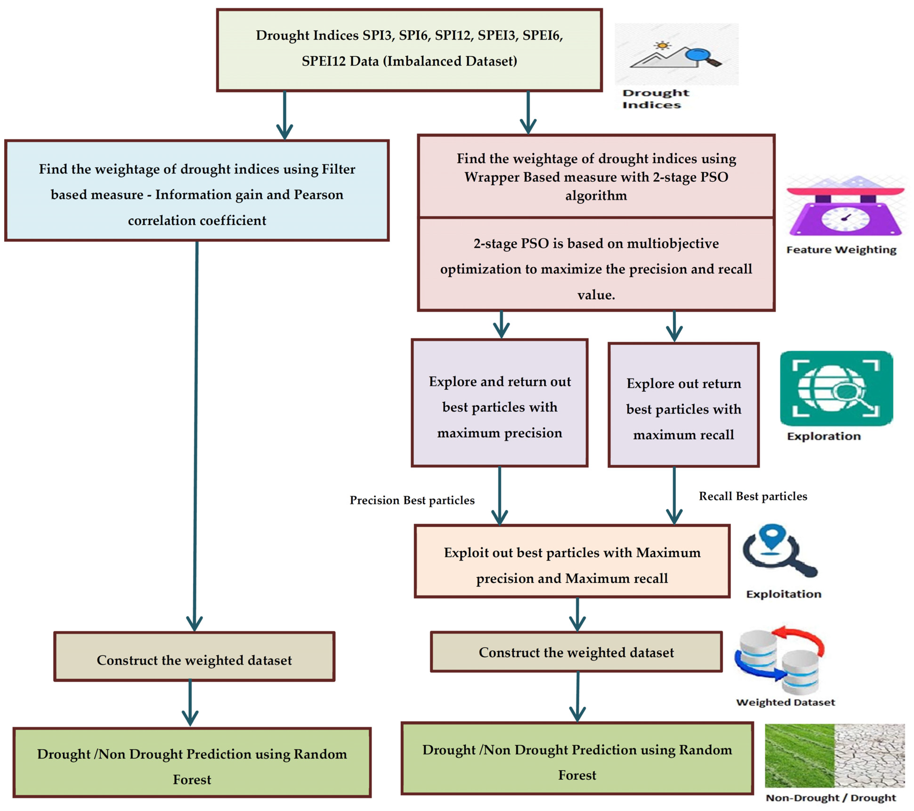
3.2. Methodology
3.2.1. Global-Filter-Supervised Feature Weighting
| Algorithm 1. Pseudocode for weighted dataset construction |
| Input: Features F = [Month, SPI 3, SPI 6, SPI 12, SPEI 3, SPEI 6, SPEI 12] Weight of features W = [w1, w2, w3, w4, w5, w6, w7] Output: F′ij represents the weighted feature value of the ith feature for the jth month with weight wi Auxiliary Variables: ‘i’ represents Features numbering from 1 to 7 ‘j’ represents Months from Jan-1950 to Dec-2012 Fij represents the feature value of the ith feature for the jth month Wi represents the weight calculated for the ith feature Intialization: IG[ ] = Information gain value for Feature in F[ ] PCW[ ] = Pearson correlation coefficient for the Feature in F[ ] PSOWT[ ] = Particle position values, given by PSO 2-stage for the Feature in F[ ] Begin: WeightedDatasetConstruction(W[ ]){
|
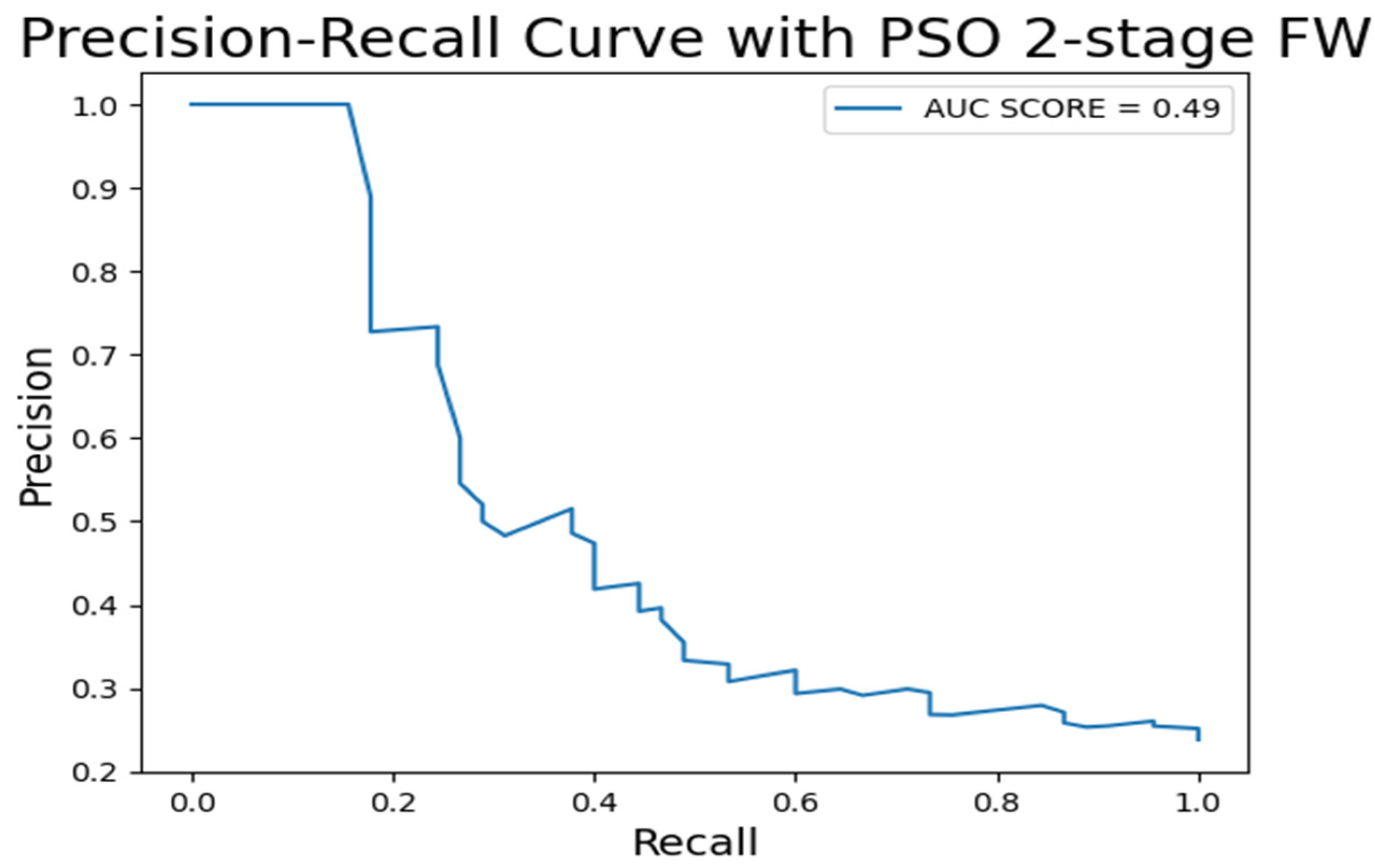
3.2.2. Global-Wrapper-Supervised Feature Weighting
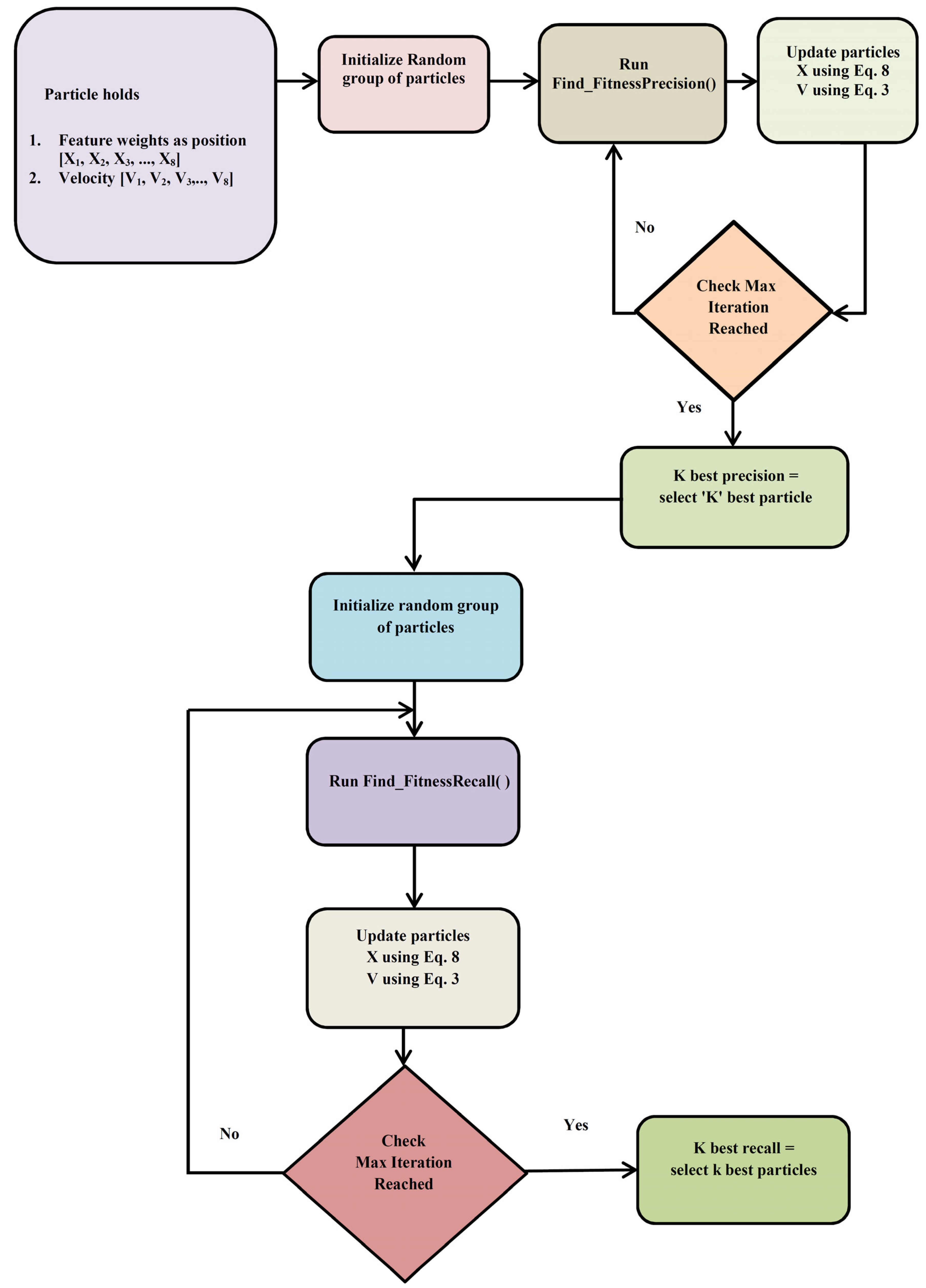
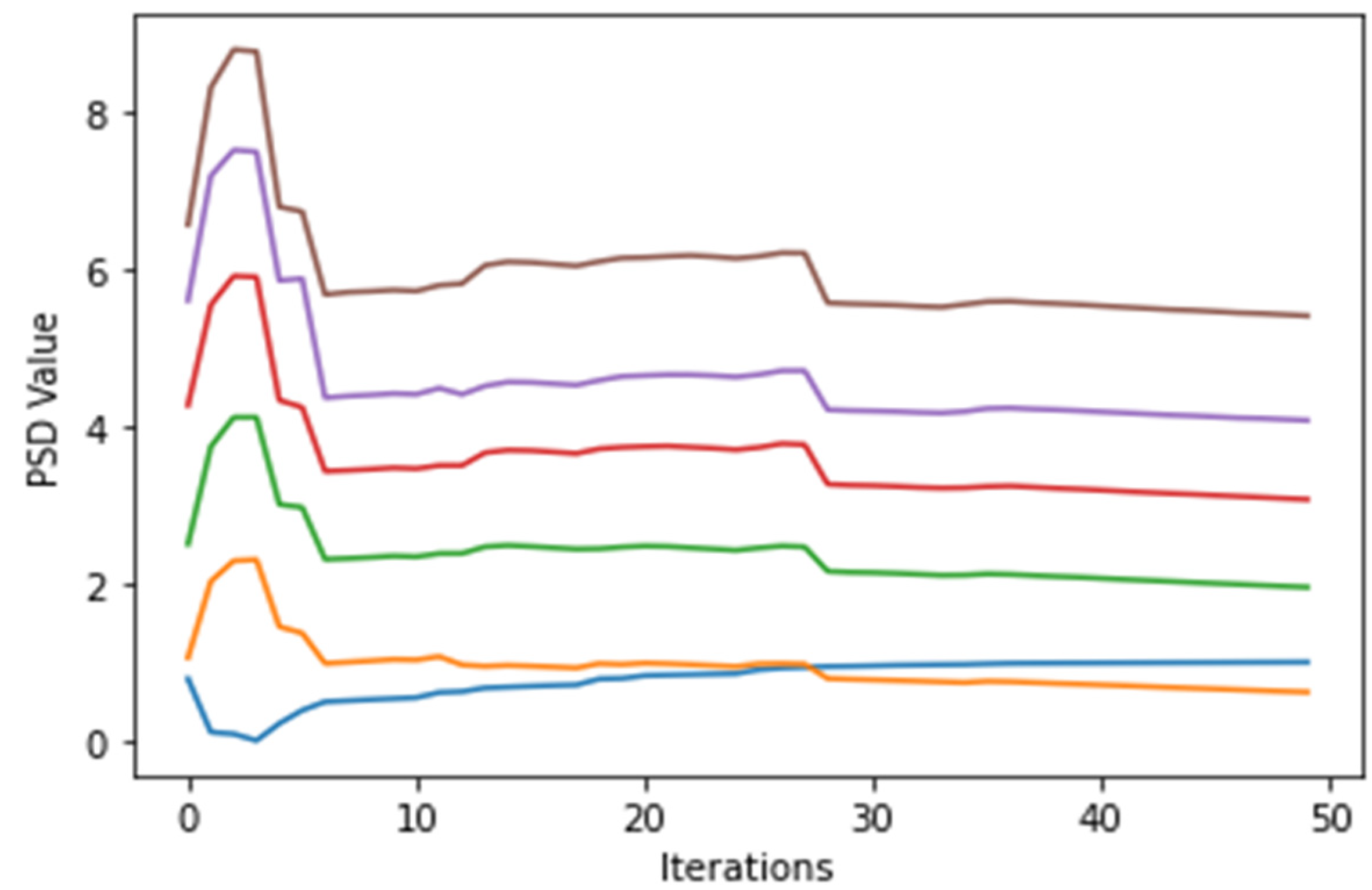
3.3. Two-Stage PSO Algorithm (PSO 2-Stage)
- Wmax = 0.9
- wmin = 0.2
- wi = weight at iteration ‘I’
- max_iteration = Maximum Iteration
- X—Particle Position
- w—Inertia weight
- V—Velocity of the particle
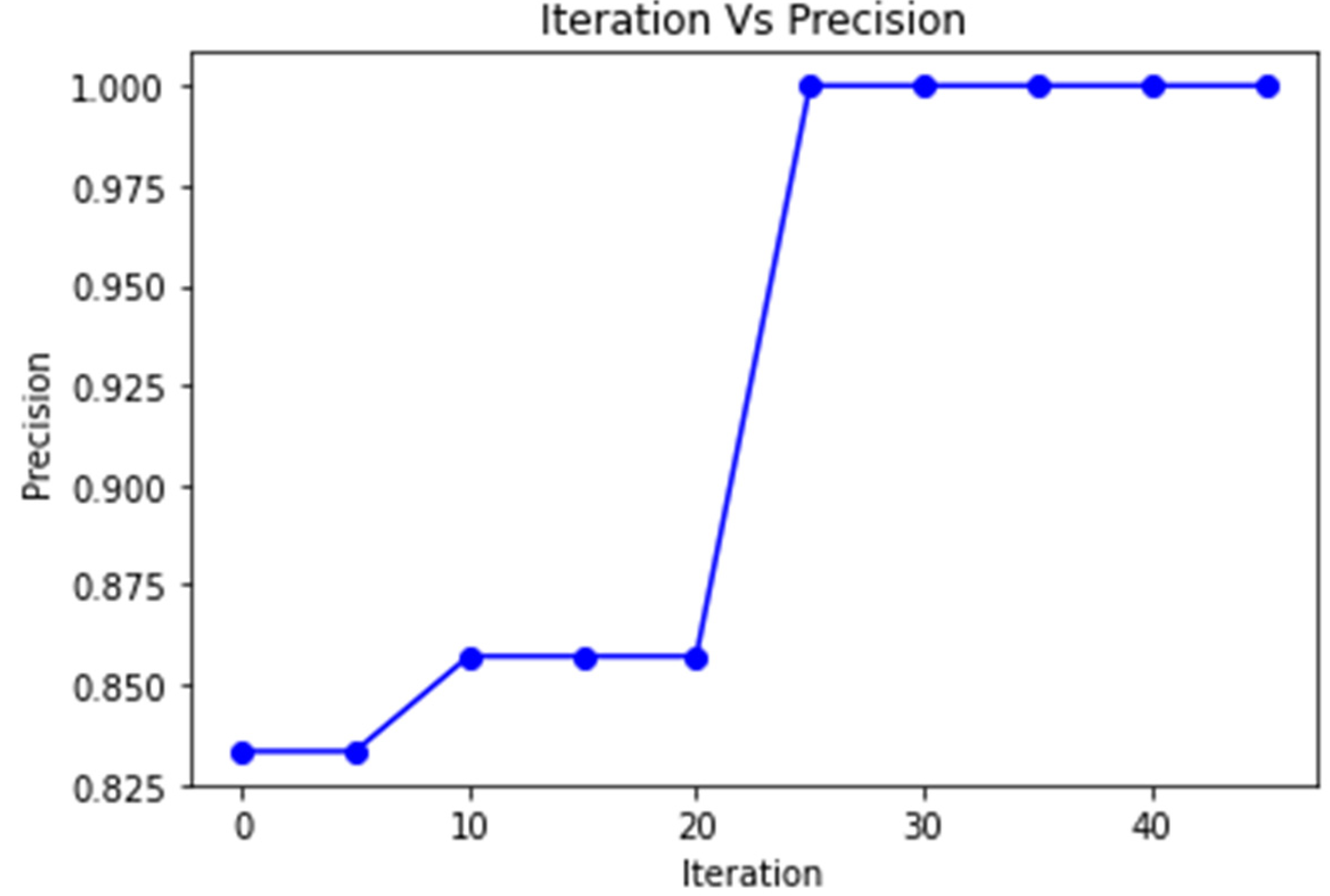
3.3.1. Exploration Phase (Stage 1 Process)
| Algorithm 2. Pseudocode for PSO Stage 1 |
| Input: S, D, Max_Iter, Particle P, Velocity V, Position X Output: Position X = [X1, X2XD] //Position—Represents the weightage of the features Auxiliary Variables: Iter = 0,fval_precision, Precision_Above75, fval_Recall, Recall_Above1, pBest, gBest Intialization: S = Population Size, D = Dimension, Max_Iter = Maximum Iteration, Initialize the particles P with a random population P = [P1, P2, P3PS], Velocity V = [V1, V2, V3VD], Position X = [X1, X2XD] Begin: PSO Stage 1 Algorithm |
// Construction of particle population with the best precision
|
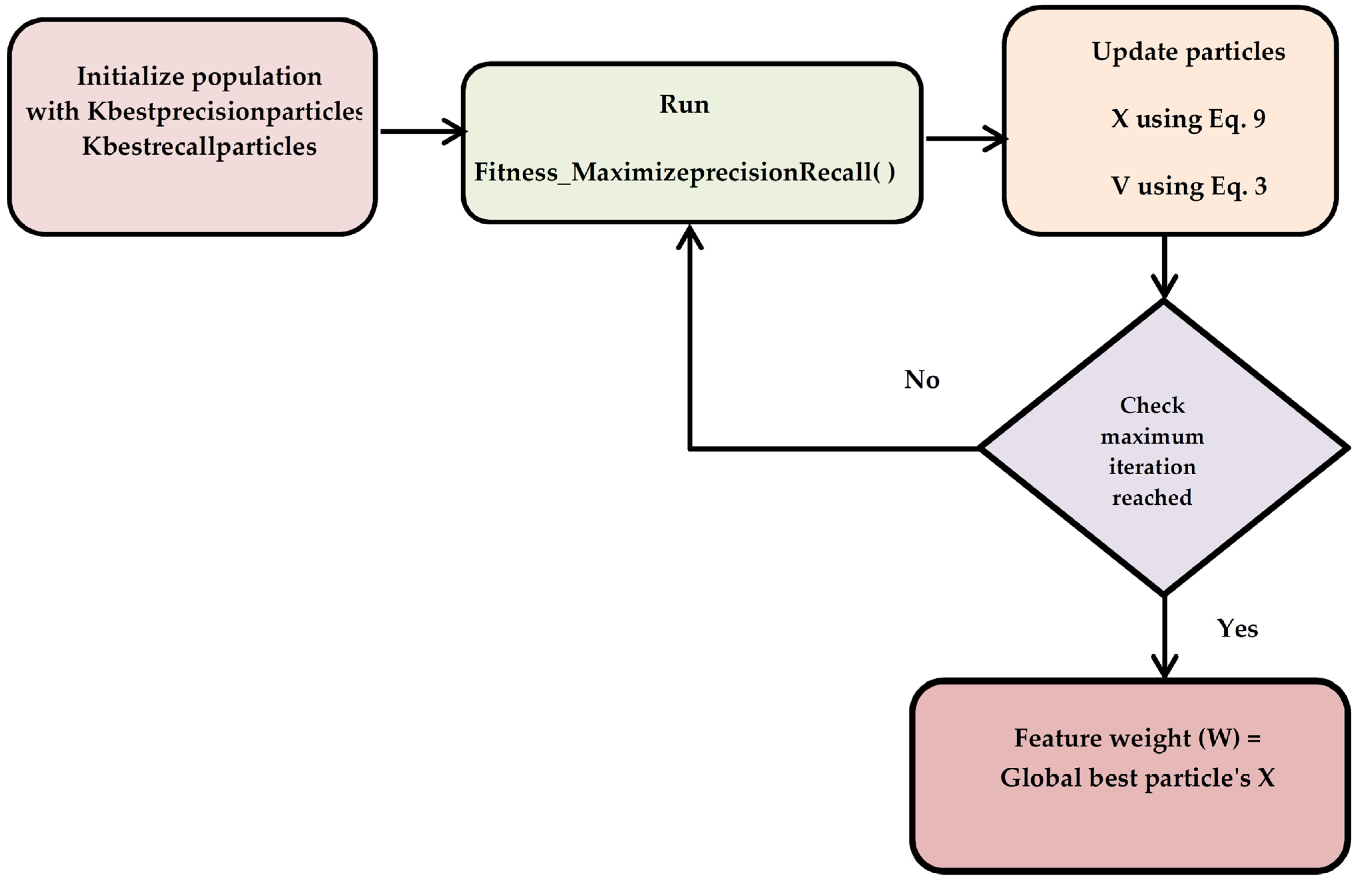
3.3.2. Exploitation Phase (Stage 2 Process)
| Algorithm 3. Pseudocode for PSO Stage 2 |
| Input: Initial Population P, Velocity V, Position X Output: Position X = [X1, X2…XD] //Position—Represents the weightage of the features Auxiliary Variables: pBest_Precision, pBest_Recall, gBestparticle Intialization: Initial Population P = [{precision_Above75} U {Recall_Above1}], Iter = 0, Position X = [X1, X2…XD], Velocity V = [V1, V2, V3…VD] Begin: PSO Stage 2 Algorithm
|
4. Results and Discussion
- popmin—Minimum Position value in Population
- popmax—Maximum Position value in Population
5. Conclusions
Author Contributions
Funding
Institutional Review Board Statement
Informed Consent Statement
Data Availability Statement
Conflicts of Interest
References
- Mishra, A.K.; Singh, V.P. A review of drought concepts. J. Hydrol. 2010, 391, 202–216. [Google Scholar]
- Amin, Z.; Rehan, S.; Bahman, N.; Faisal, K. A review of drought indices. Environ. Rev. 2011, 19, 333–349. [Google Scholar]
- Edwards, D.C. Characteristics of 20th Century Drought in the United States at Multiple Time Scales; Air Force Inst of Tech Wright-Patterson: Hobson Way, OH, USA, 1997; No. AFIT-97-051. [Google Scholar]
- Beguería, S.; Vicente-Serrano, S.M.; Reig, F.; Latorre, B. Standardized precipitation evapotranspiration index (SPEI) revisited: Parameter fitting, evapotranspiration models, tools, datasets and drought monitoring. Int. J. Climatol. 2014, 34, 3001–3023. [Google Scholar]
- Bouaguel, W.; Mufti, G.B.; Limam, M. A fusion approach based on wrapper and filter feature selection methods using majority vote and feature weighting. In Proceedings of the International Conference on Computer Applications Technology (ICCAT), Sousse, Tunisia, 20–22 January 2013. [Google Scholar]
- Niño-Adan, I.; Manjarres, D.; Landa-Torres, I.; Portillo, E. Feature Weighting Methods: A Review. Expert Syst. Appl. 2021, 184, 115424. [Google Scholar]
- Jankowski, N.; Usowicz, K. Analysis of feature weighting methods based on feature ranking methods for classification. In Proceedings of the International Conference on Neural Information Processing, Shanghai, China, 13–17 November 2011. [Google Scholar]
- Wu, X.; Xu, X.; Liu, J.; Wang, H.; Hu, B.; Nie, F. Supervised feature selection with orthogonal regression and feature weighting. IEEE Trans. Neural Netw. Learn. Syst. 2021, 32, 1831–1838. [Google Scholar]
- Agrawal, P.; Abutarboush, H.F.; Ganesh, T.; Mohamed, A.W. Metaheuristic algorithms on feature selection: A survey of one decade of research (2009–2019). IEEE Access 2021, 9, 26766–26791. [Google Scholar]
- Valdez, F.; Castillo, O.; Melin, P. Bio-Inspired Algorithms and Its Applications for Optimization in Fuzzy Clustering. Algorithms 2021, 14, 122. [Google Scholar]
- Kennedy, J.; Eberhart, R. Particle Swarm Optimization. In Proceedings of the IEEE International Conference on Neural Networks, Perth, WA, Australia, 27 November–1 December 1995. [Google Scholar]
- Shami, T.M.; El-Saleh, A.A.; Alswaitti, M.; Al-Tashi, Q.; Summakieh, M.A.; Mirjalili, S. Particle swarm optimization: A comprehensive survey. IEEE Access 2022, 10, 10031–10061. [Google Scholar]
- Eberhart, R.C.; Shi, Y. Particle Swarm Optimization: Developments, Applications and Resources. In Proceedings of the IEEE Congress on Evolutionary Computation, Seoul, Republic of Korea, 27–30 May 2001; Volume 1, pp. 27–30. [Google Scholar]
- Jiang, L.; Zhang, L.; Li, C.; Wu, J. A Correlation-based Feature Weighting Filter for Naive Bayes. IEEE Trans. Knowl. Data Eng. 2018, 31, 201–213. [Google Scholar]
- Khadr, M. Forecasting of meteorological drought using Hidden Markov Model (case study: The upper Blue Nile river basin, Ethiopia). Ain. Shams. Eng. J. 2016, 7, 47–56. [Google Scholar]
- Dikshit, A.; Pradhan, B.; Huete, A. An improved SPEI drought forecasting approach using the long short-term memory neural network. J. Environ. Manag. 2021, 283, 111979. [Google Scholar]
- Zhang, R.; Chen, Z.Y.; Xu, L.J.; Ou, C.Q. Meteorological drought forecasting based on a statistical model with machine learning techniques in Shaanxi province, China. Sci. Total Environ. 2019, 665, 338–346. [Google Scholar]
- Mathivha, F.; Sigauke, C.; Chikoore, H.; Odiyo, J. Short-Term and Medium-Term Drought Forecasting Using Generalized Additive Models. Sustainability 2020, 12, 4006. [Google Scholar]
- Pande, C.B.; Al-Ansari, N.; Kushwaha, N.L.; Srivastava, A.; Noor, R.; Kumar, M.; Moharir, K.N.; Elbeltagi, A. Forecasting of SPI and Meteorological Drought Based on the Artificial Neural Network and M5P Model Tree. Land 2022, 11, 2040. [Google Scholar] [CrossRef]
- Ndayiragije, J.M.; Li, F.; Nkunzimana, A. Assessment of Two Drought Indices to Quantify and Characterize Drought Incidents: A Case Study of the Northern Part of Burundi. Atmosphere 2022, 13, 1882. [Google Scholar] [CrossRef]
- Yang, W.; Zhou, X.; Luo, Y. Simultaneously Optimizing Inertia Weight and Acceleration Coefficients via Introducing New Functions into PSO Algorithm. J. Phys. Conf. Ser. 2021, 1754, 012195. [Google Scholar]
- Zhang, L.; Tang, Y.; Hua, C.; Guan, X. A new particle swarm optimization algorithm with adaptive inertia weight based on Bayesian techniques. Appl. Soft Comput. 2015, 28, 138–149. [Google Scholar]
- Liang, H.; Kang, F. Adaptive mutation particle swarm algorithm with dynamic nonlinear changed inertia weight. Optik 2016, 127, 8036–8042. [Google Scholar]
- Kadirkamanathan, V.; Selvarajah, K.; Fleming, P.J. Stability analysis of the particle dynamics in particle swarm optimizer. IEEE Trans. Evol. Comput. 2006, 10, 245–255. [Google Scholar]
- Pluhacek, M.; Senkerik, R.; Davendra, D.; Oplatkova, Z.K.; Zelinka, I. On the behavior and performance of chaos driven PSO algorithm with inertia weight. Comput. Math. Appl. 2013, 66, 122–134. [Google Scholar]
- Li, W.; Meng, X.; Huang, Y.; Fu, Z.H. Multipopulation cooperative particle swarm optimization with a mixed mutation strategy. Inform. Sci. 2020, 529, 179–196. [Google Scholar]
- Ye, W.; Feng, W.; Fan, S. A novel multi-swarm particle swarm optimization with dynamic learning strategy. Appl. Soft Comput. J. 2017, 61, 832–843. [Google Scholar]
- Tripathy, B.K.; Reddy Maddikunta, P.K.; Pham, Q.V.; Gadekallu, T.R.; Dev, K.; Pandya, S.; ElHalawany, B.M. Harris Hawk Optimization: A Survey on Variants and Applications. Comput. Intell. Neurosci. 2022, 2022, 2218594. [Google Scholar]
- Reddy, G.T.; Reddy, M.P.K.; Lakshmanna, K.; Kaluri, R.; Rajput, D.S.; Srivastava, G.; Baker, T. Analysis of Dimensionality Reduction Techniques on Big Data. IEEE Access 2020, 8, 54776–54788. [Google Scholar]
- Available online: https://rda.ucar.edu/datasets/ds298.0/index.html#!cgi-bin/datasets/getWebList?dsnum=298.0 (accessed on 23 September 2022).
- Available online: https://spei.csic.es/spei_database/ (accessed on 30 September 2022).
- Available online: https://digitalcommons.unl.edu/droughtnetnews/57/ (accessed on 15 September 2022).
- Elhariri, E.; El-Bendary, N.; Taie, S.A. Using Hybrid Filter-Wrapper Feature Selection With Multi-Objective Improved-Salp Optimization for Crack Severity Recognition. IEEE Access 2020, 8, 84290–84315. [Google Scholar]
- Lei, S. A feature selection method based on information gain and genetic algorithm. In Proceedings of the 2012 International Conference on Computer Science and Electronics Engineering, Hangzhou, China, 23–25 March 2012; Volume 2, pp. 355–358. [Google Scholar]
- Yang, M.; Liu, Y.; Yang, J. A hybrid multi-objective particle swarm optimization with central control strategy. Comput. Intell. Neurosci. 2022, 2022, 1522096. [Google Scholar]
- Ekbalm, A.; Saha, S.; Garbe, C. Feature selection using multiobjective optimization for named entity recognition. In Proceedings of the 20th International Conference on Pattern Recognition (ICPR), Istanbul, Turkey, 23–26 August 2010; pp. 1937–1940. [Google Scholar]
- Wei, B.; Xia, X.; Yu, F.; Zhang, Y.; Xu, X.; Wu, H.; Gui, L.; He, G. Multiple adaptive strategies based particle swarm optimization algorithm. Swarm Evolut. Comput. 2020, 57, 100731. [Google Scholar]
- Lim, W.H.; Isa, N.A.M. An adaptive two-layer particle swarm optimization with elitist learning strategy. Inf. Sci. 2014, 273, 49–72. [Google Scholar]
- Taherkhani, M.; Safabakhsh, R. A novel stability-based adaptive inertia weight for particle swarm optimization. Appl. Soft Comput. 2016, 38, 281–295. [Google Scholar]
- Liu, H.; Zhang, X.-W.; Tu, L.-P. A Modified Particle Swarm Optimization Using Adaptive Strategy. Expert Syst. Appl. 2020, 152, 113353. [Google Scholar]


| S. No. | SPI/SPEI Value | Drought Severity Level |
|---|---|---|
| 1 | Greater than 2 | Extremely wet |
| 2 | 1.5 to 2 | Very wet |
| 3 | 1 to 1.4 | Moderately wet |
| 4 | −1 to 0.9 | Normal |
| 5 | −1.5 to −1.1 | Moderately dry |
| 6 | −2 to −1.6 | Severely dry |
| 7 | values below −2 | Extremely dry |
| S.No. | Author | Data Used | Contributions | Shortcomings |
|---|---|---|---|---|
| 1 | Mosaad Khadr [15] | Precipitation data, LST, NDVI, and soil moisture. | The short to medium term SPI was forecasted using different types of homogenous hidden Markov models. Real-time multivariate Madden–Julian oscillation (RMM MJO) index-based model predicts well using the random forest. Good in forecasting SPI for various time-series one month ahead. | The one-month lead time prediction performance of SPI3, SPI6, SPI12 is comparatively lower than other leadtimes. SPI12 prediction shows a minimum RMSE value. |
| 2 | Dikshit [16] | SPEI1, SPEI3, hydro-metrological variables, namely, rainfall, maximum temperature, minimum temperature, mean temperature, vapour pressure, and cloud cover. | The SPEI1 and SPEI3 prediction using long short-term memory (LSTM) was done. One LSTM Layer and one dense layer are used and with the performance metrics coefficient of determination and root mean square error, the model is evaluated. Spatial analysis is also performed in addition to the statistical measures | Experiments were not carried out on longer timescales. Interpretation of the results achieved has to be completed. |
| 3 | Zhang [17] | Seasons, metrological factors, and climatic indicators. | The features used in SPEI1, SPEI3, SPEI6, and SPEI12 prediction are evaluated using the cross-correlation function and a distributed lag nonlinear model (DLNM) methods. Then the SPEI1–6 forecasting was executed using DLNM, an artificial neural network model and an XGBoost model. The forecasting results are compared and the highest prediction accuracy was returned by XGBoost model. | Instead of solar radiation data, the sunshine hour was considered. Making use of tree boosters will give better results. |
| 4 | Mathivha [18] | SPEI with PET was calculated using Hagreaves’ and Samani’s temperature-based method. | Time series decomposition was performed as a preprocessing step in SPEI1, SPEI6, and SPEI12 prediction with generalized additive model (GAM), GAM integration with ensemble empirical mode decomposition, and autoregressive integrated moving average (ARIMA), and forecast quantile regression averaging (fQRA) as classifiers. The fQRA forecast was best at forecasting 12 month scale. | Decomposition does not give great improvements in one-month time scale. |
| 5 | Pande Chaitanya [19] | SPI | The SPI3 and SPI6 prediction was performed with ANN and M5P for the Maharastra State of India. The number of SPI of varying timescale combinations suitable for SPI3 and SPI6 are 7 and 4. M5P returns the best RMSE value. | The metrological drought determination is done based on the SPI value alone. |
| 6 | Jean Marie [20] | SPI and SPEI | The SPI and SPEI effectiveness is compared for the mountainous and plateau region present in the northern part of Burundi. The timescales of 2,4,24 and 48 are used. The results show that SPEI is a better measure for meteorological data than SPI. | The author also suggests the usage of multiple drought indices in predicting drought. |
| Wrapper Algorithms | Drought Precision | Drought Recall | Drought F1Score | Non Drought F1score | Non Drought Precision | Non Drought Recall | Matthews Correlation Coefficient |
|---|---|---|---|---|---|---|---|
| Naïve Bayesian | 0.24 | 0.18 | 0.21 | 0.79 | 0.76 | 0.83 | 0.0046 |
| Logistic Regression | 0.50 | 0.02 | 0.04 | 0.86 | 0.76 | 0.99 | 0.0635 |
| Random Forest | 0.88 | 0.20 | 0.33 | 0.89 | 0.81 | 0.99 | 0.367 |
| Method | Drought Precision | Drought Recall | Drought F1Score | Non Drought F1score | Non Drought Precision | Non Drought Recall | Accuracy | Matthews Correlation Coefficient |
|---|---|---|---|---|---|---|---|---|
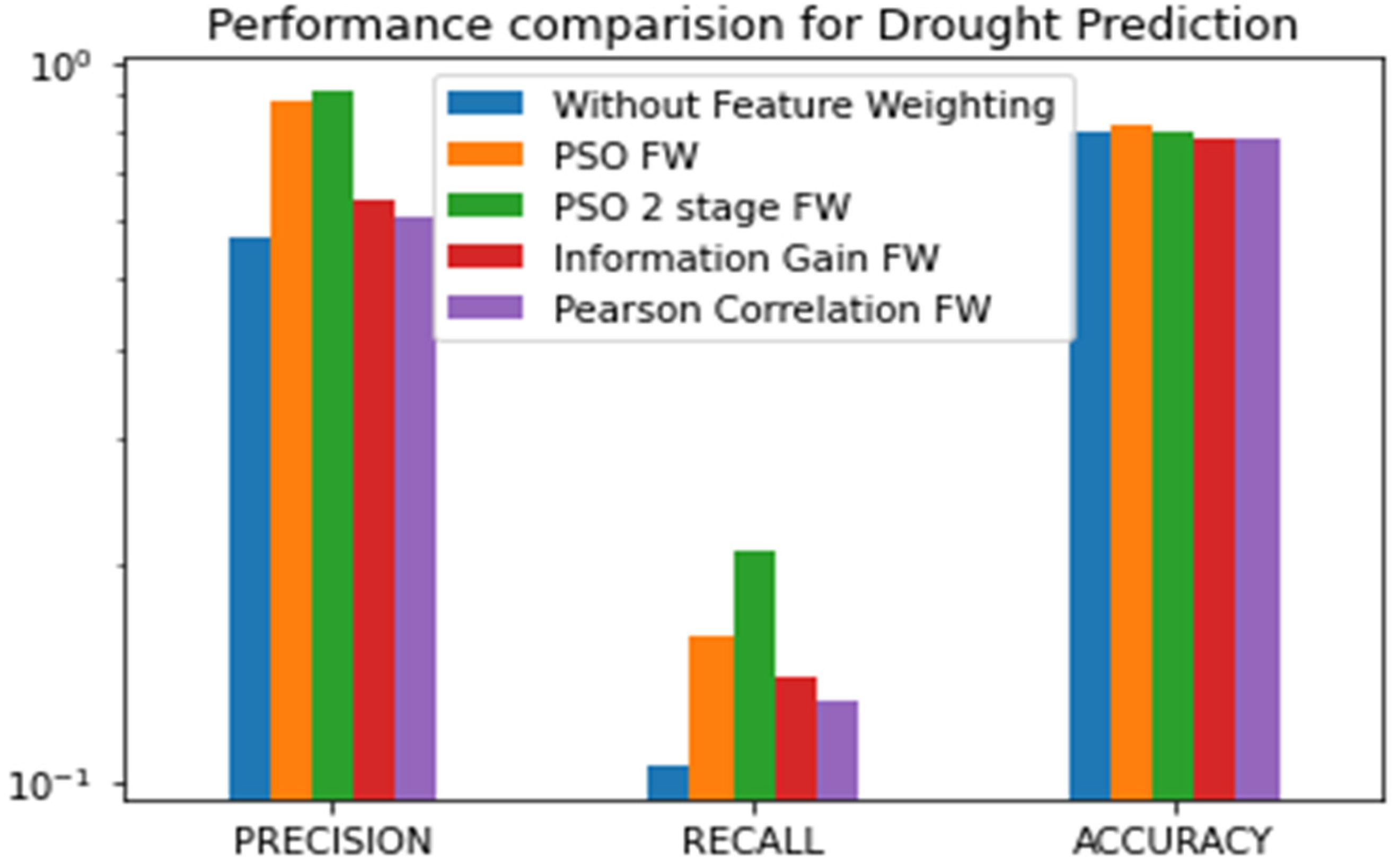
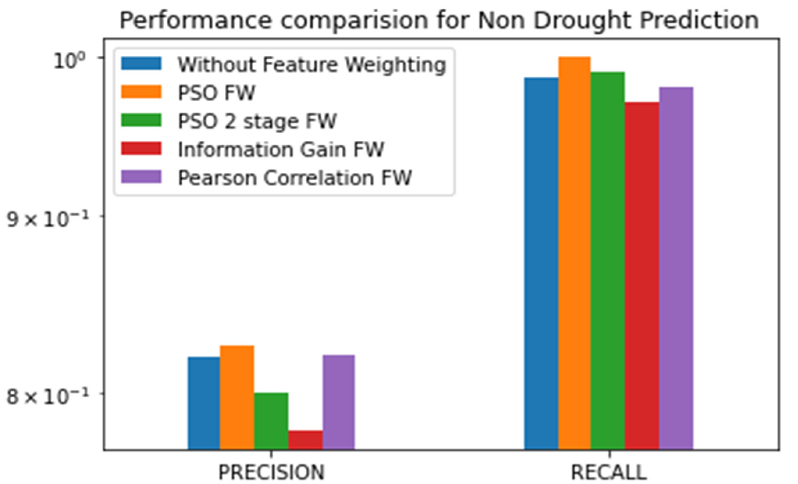
| Without FW | 0.55 | 0.1 | 0.21 | 0.89 | 0.81 | 0.97 | 0.79 | 0.15 |
| Information Gain FW | 0.64 | 0.14 | 0.18 | 0.89 | 0.78 | 0.97 | 0.78 | 0.18 |
| Pearson Correlation FW | 0.61 | 0.13 | 0.26 | 0.92 | 0.82 | 0.98 | 0.78 | 0.32 |
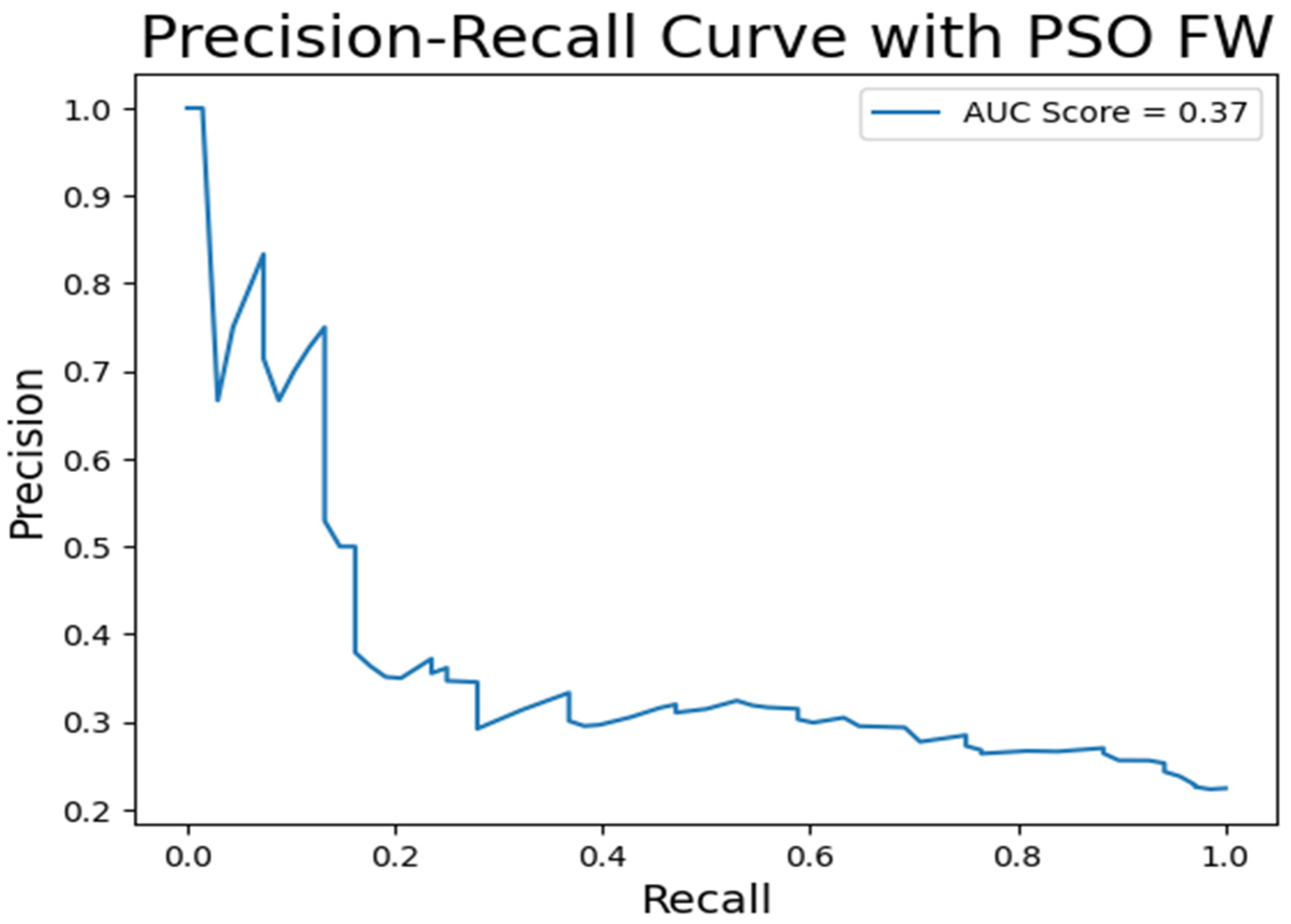
| PSO FW | 0.88 | 0.16 | 0.33 | 0.89 | 0.81 | 0.99 | 0.82 | 0.36 |
| PSO 2-Stage FW | 1 | 0.21 | 0.37 | 0.88 | 0.82 | 0.99 | 0.8 | 0.38 |
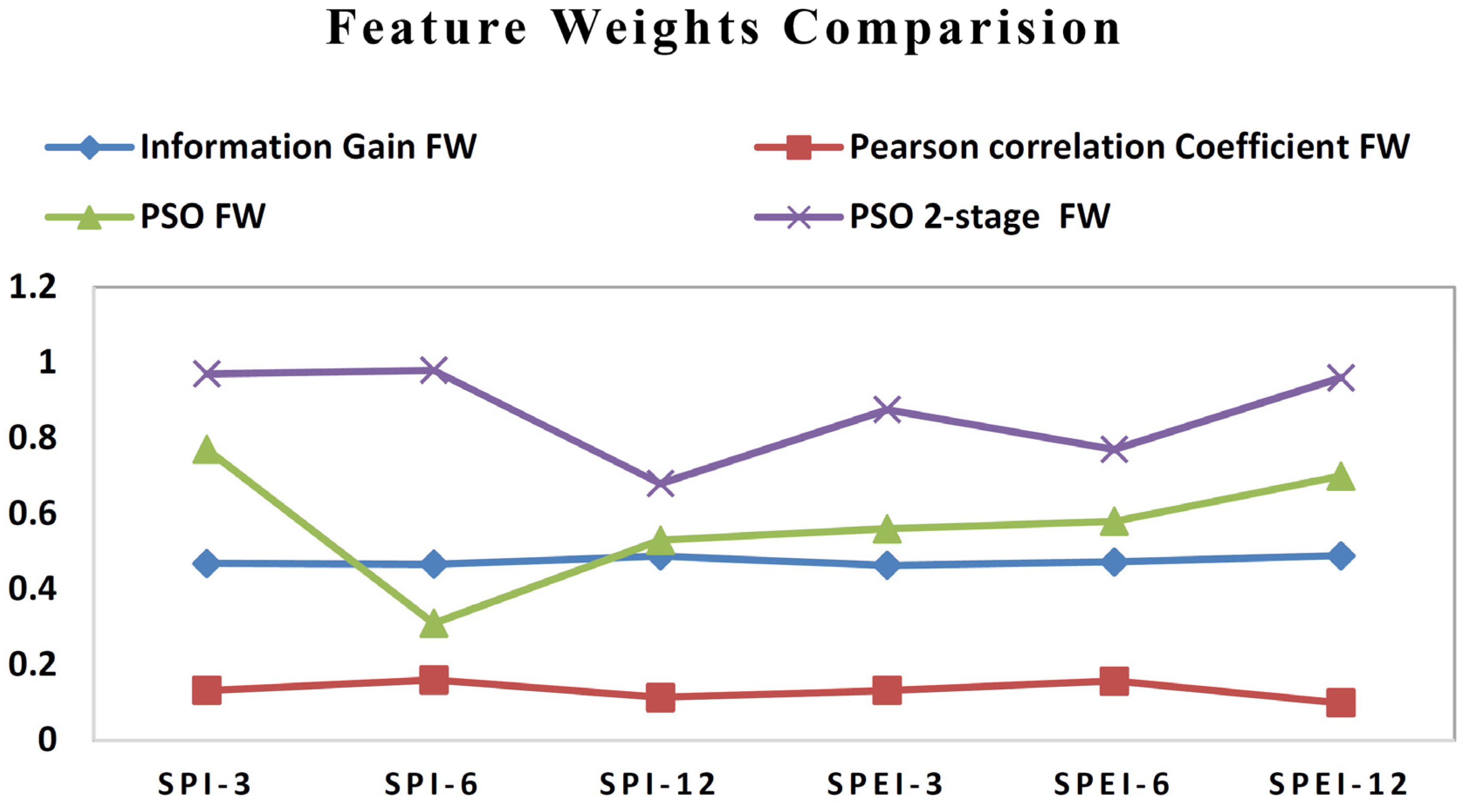
| S. No. | Feature Weighting Methods | SPI 3 | SPI 6 | SPI 12 | SPEI 3 | SPEI 6 | SPEI 12 |
|---|---|---|---|---|---|---|---|
| 1. | Information Gain FW | 0.468 | 0.466 | 0.488 | 0.463 | 0.472 | 0.489 |
| 2. | Pearson Correlation Coefficient FW | 0.132 | 0.16 | 0.113 | 0.132 | 0.157 | 0.099 |
| 3. | PSO FW | 0.77 | 0.31 | 0.53 | 0.56 | 0.58 | 0.7 |
| 4. | PSO 2-stage FW | 0.97 | 0.98 | 0.68 | 0.876 | 0.77 | 0.96 |
Disclaimer/Publisher’s Note: The statements, opinions and data contained in all publications are solely those of the individual author(s) and contributor(s) and not of MDPI and/or the editor(s). MDPI and/or the editor(s) disclaim responsibility for any injury to people or property resulting from any ideas, methods, instructions or products referred to in the content. |
© 2023 by the authors. Licensee MDPI, Basel, Switzerland. This article is an open access article distributed under the terms and conditions of the Creative Commons Attribution (CC BY) license (https://creativecommons.org/licenses/by/4.0/).
Share and Cite
Sundararajan, K.; Srinivasan, K. Feature-Weighting-Based Prediction of Drought Occurrence via Two-Stage Particle Swarm Optimization. Sustainability 2023, 15, 929. https://doi.org/10.3390/su15020929
Sundararajan K, Srinivasan K. Feature-Weighting-Based Prediction of Drought Occurrence via Two-Stage Particle Swarm Optimization. Sustainability. 2023; 15(2):929. https://doi.org/10.3390/su15020929
Chicago/Turabian StyleSundararajan, Karpagam, and Kathiravan Srinivasan. 2023. "Feature-Weighting-Based Prediction of Drought Occurrence via Two-Stage Particle Swarm Optimization" Sustainability 15, no. 2: 929. https://doi.org/10.3390/su15020929
APA StyleSundararajan, K., & Srinivasan, K. (2023). Feature-Weighting-Based Prediction of Drought Occurrence via Two-Stage Particle Swarm Optimization. Sustainability, 15(2), 929. https://doi.org/10.3390/su15020929