Biomass Estimation of Subtropical Arboreal Forest at Single Tree Scale Based on Feature Fusion of Airborne LiDAR Data and Aerial Images
Abstract
1. Introduction
2. Materials and Methods
2.1. Study Area
2.2. Field Data Collection
2.3. UAV Data Collection
2.4. Data Preprocessing
2.4.1. Preprocessing of Image and Point Cloud
2.4.2. Segmentation in Single Tree Scale and Classification of Dominant Species
2.4.3. Spectral Features Extraction of the Images
- (1)
- Spectral and visible light vegetation index feature extraction
- (2)
- Image texture feature extraction
2.4.4. Structural Features Extraction of Point Cloud
2.4.5. Canopy and Topographic Features Extraction
2.5. Statistical Analysis
2.5.1. Correlation Analysis
2.5.2. Permutation Importance Index Analysis
2.6. Modeling
2.6.1. Random Forest
2.6.2. XGBoost
2.6.3. Grid Search
2.6.4. Experimental Environment
2.6.5. Model Evaluation Method
3. Results
3.1. Biomass Statistical Analysis of Tree Species Samples
3.2. Feature Analysis
3.2.1. Correlation Analysis
3.2.2. Permutation Importance Index of Features
3.3. Range of Grid Search Parameters
3.4. Model Construction and Evaluation using Original Feature Combinations
3.5. Model Construction and Evaluation Using Filtered Features
3.6. Mapping of Biomass in The Study Area
4. Discussion
- (1)
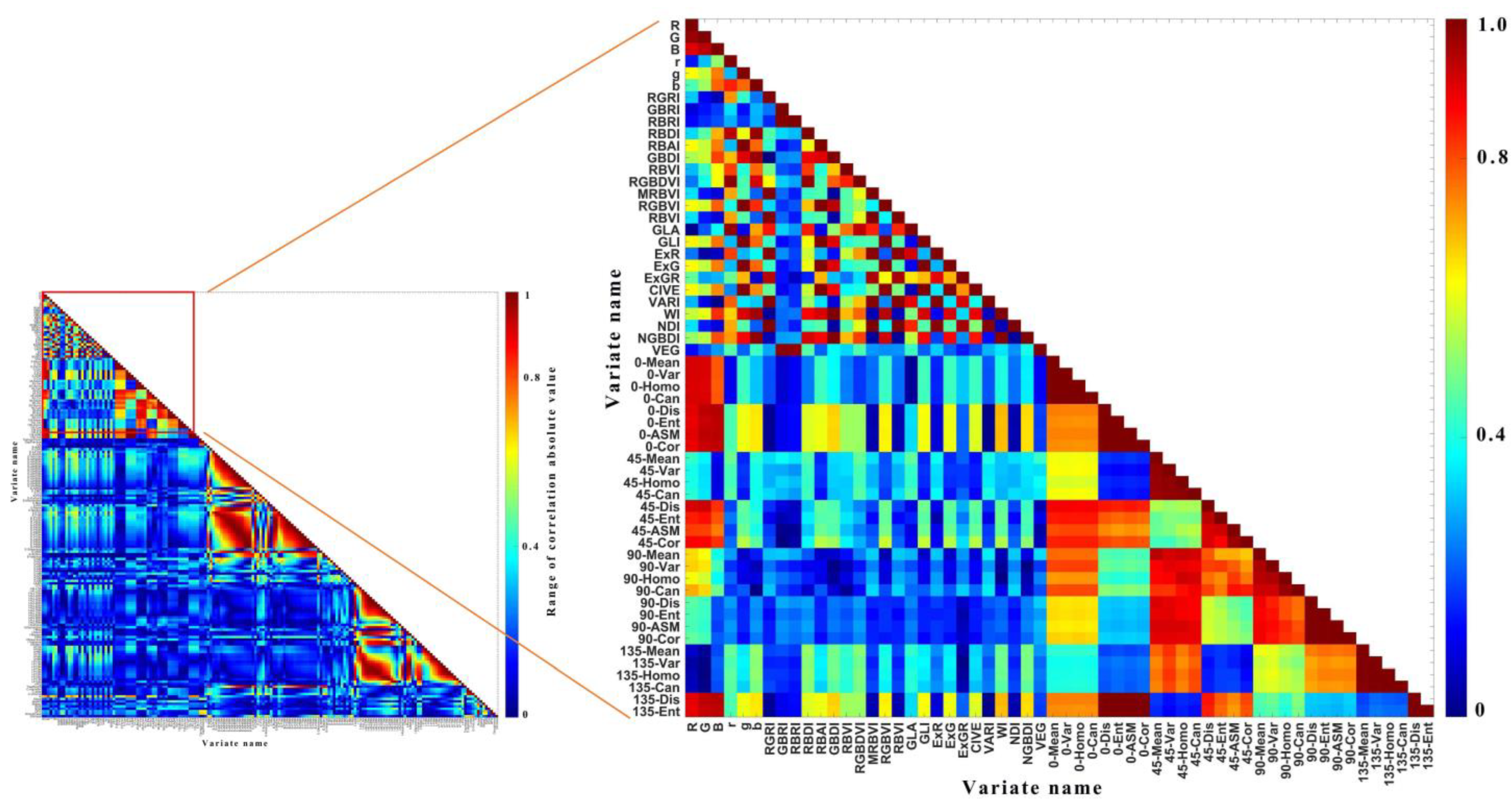
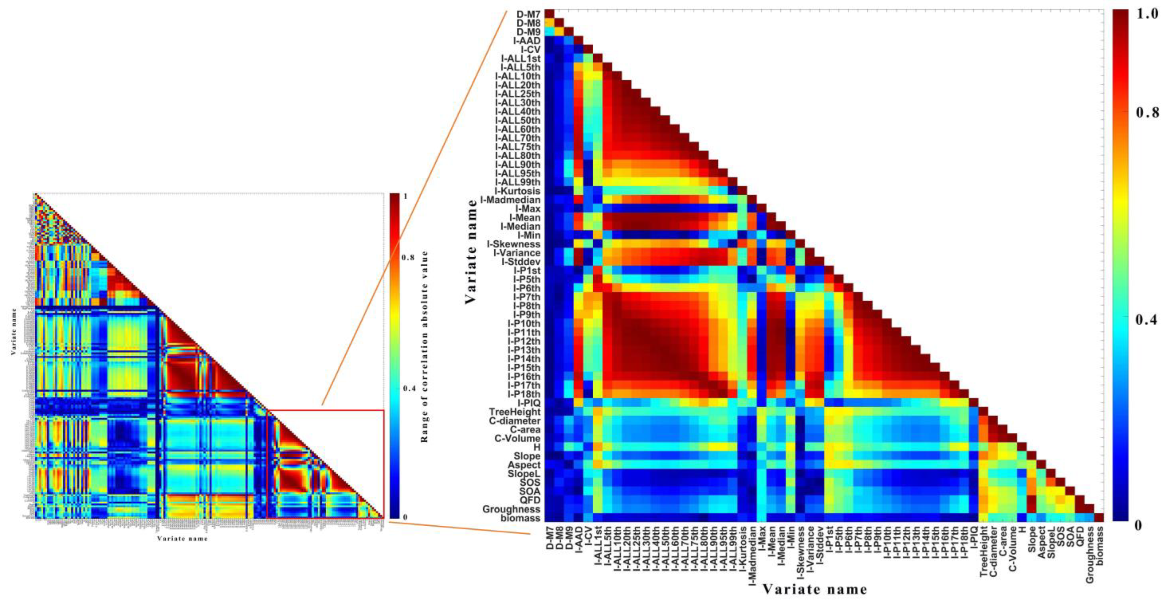
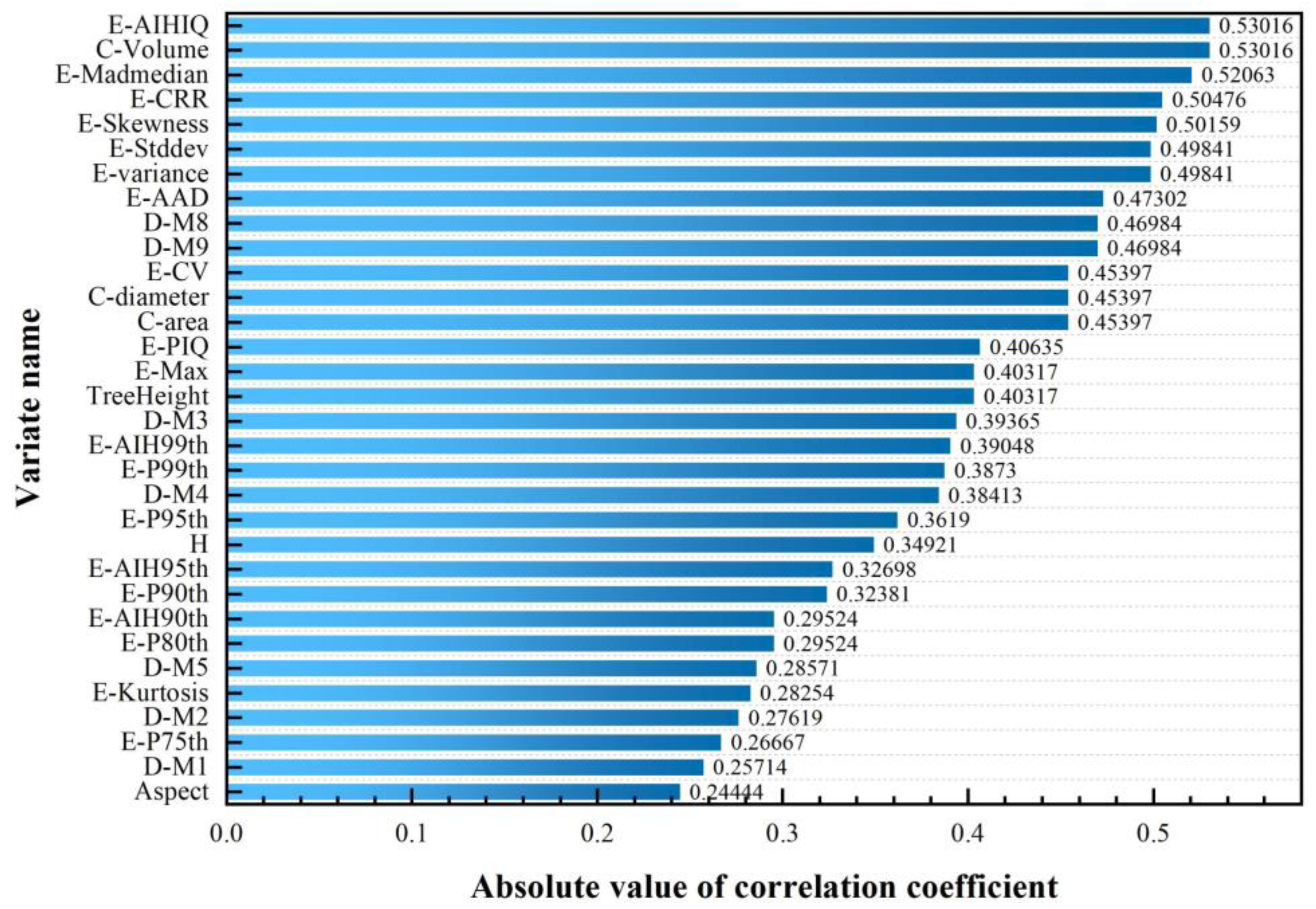
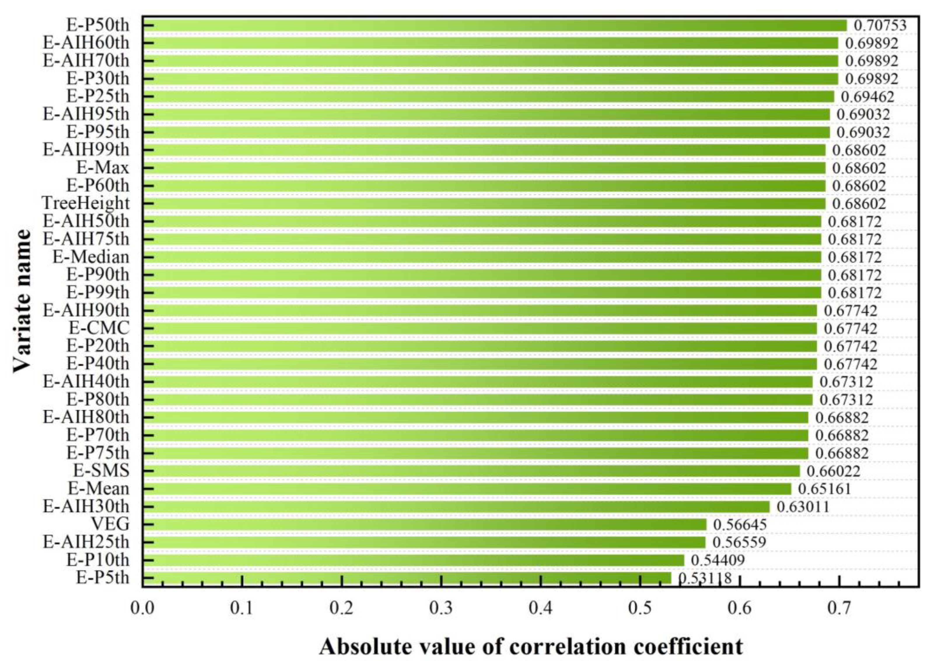
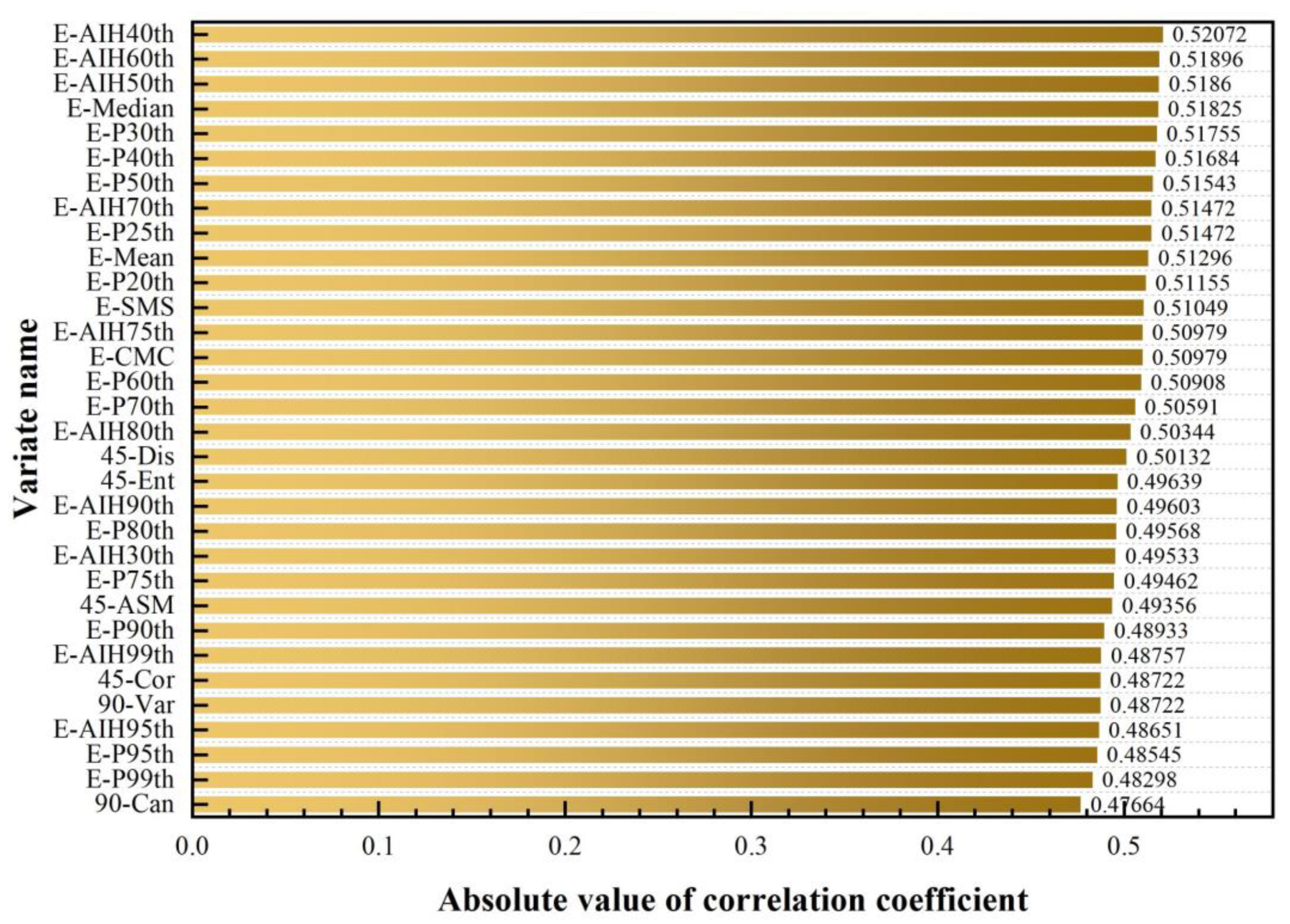
- There were significant differences in the correlation and important features among different tree species. The point cloud height, canopy, and topographic features were all of high importance in the three tree species and were basically consistent with some previous research conclusions [26,27,40]. Among them, the point cloud height percentile, cumulative percentile, canopy volume, tree height, and ground elevation as individual variables showed outstanding PI importance scores. The difference is that the features of the point cloud density and intensity are only of particular importance for the Cupressus lusitanica and the image texture features are only important for Deciduous Broad-leaved Forest.
- (2)
- The estimation accuracy of RF and XGBoost models cannot be improved by eliminating the multicollinearity problem among variables. This feature-selection processing method has shown to be beneficial in the biomass estimation of linear models in the past [41,42]. However, for machine learning models that handle high-dimensional data well, such as RF and XGBoost, the sampling of features and samples can be adopted to avoid multicollinearity problems. At the same time, this processing will greatly reduce the diversity of the decision trees, which can affect the estimation accuracy. In addition, the estimation accuracy of the permutation importance index method is better than that of the correlation analysis. This indicates the advantages of wrapper methods such as PI in feature screening. Compared with the filter method, it is more targeted and has a better effect on model improvement [43].
- (3)
- Image features such as the visible light vegetation index and texture had little influence on the biomass estimation of arboreal forests. Except for the texture features of the Deciduous Broad-leaved Forest, the image features were less correlated and important to the biomasses of the three tree species. In the feature combination experiment, the estimation accuracy was not improved much by combining the image features. This is different from the previous biomass estimation studies on annual crops such as maize, potato, and winter oilseed rape [19,20,21]. Because the spectral responses of annual crops are different in different growth stages and are associated with the accumulation process of crop biomass. The relatively accurate biomass estimation can be obtained through spectral information. Obviously, this theory is not applicable to the biomass estimation of subtropical arbor forests, whose leaf spectral responses are usually strongly correlated with seasons, but not with the growth cycle.
- (4)
- The differentiation between species is beneficial for forest biomass estimation. The best estimation accuracy was achieved for all three tree species by using the combination of the post-fusion features, permutation importance index, and random forest model. The best estimation accuracy of the three tree species in the test sets are: Cupressus lusitanica: (RMSE = 0.1176, R2 = 0.7346), Pinus yunnanensis: (RMSE = 0.0960, R2 = 0.8578), and Deciduous Broad-leaved Forest: (RMSE = 0.0986, R2 = 0.6823). Among them, the single species of Cupressus lusitanica and Pinus yunnanensis achieved significantly higher estimation accuracy than the mixed species of Subtropical Deciduous Broad-leaved Forest.
- (5)
- The biomass estimation model in this study has regional limitations. Since the true values of the sample biomass were calculated by regional bivariate biomass equations, such equations are often strictly limited to the application area and tree species. Therefore, it is very important to change the acquisition method of the biomass truth value for reference in future research.
5. Conclusions
- (1)
- In this study, the visible light vegetation index, texture, point cloud height, density, intensity, canopy, and topographic features were extracted. Among them, the point cloud height features, canopy variates, and the topographic-related factors showed great importance in the biomass estimation of the three species. In addition, the characteristics of the point cloud density and intensity are only important for Cupressus lusitanica. The image texture features are only important for the subtropical Deciduous Broad-leaved Forest. The visible light index had little effect on the biomass estimation of the three tree species.
- (2)
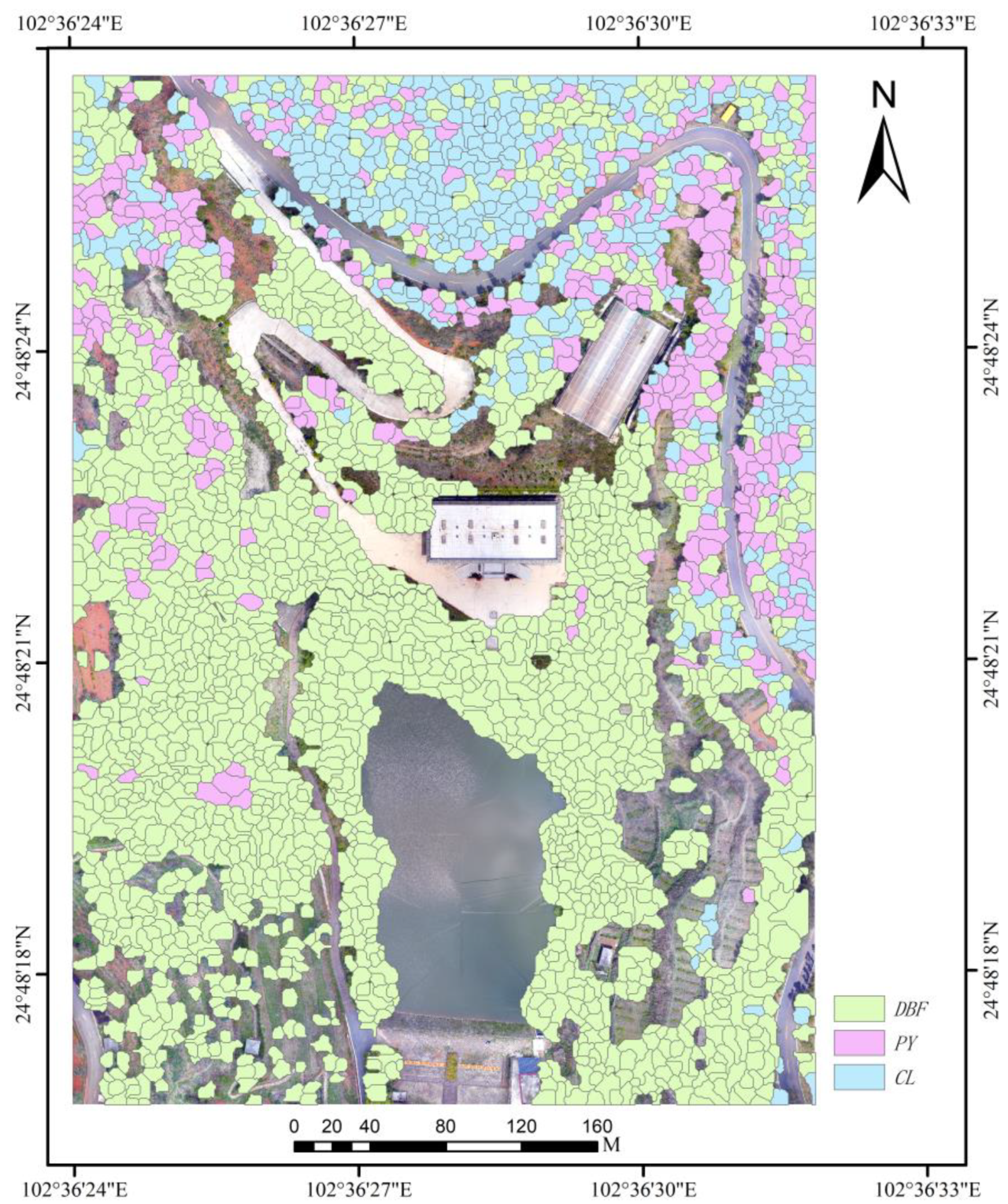
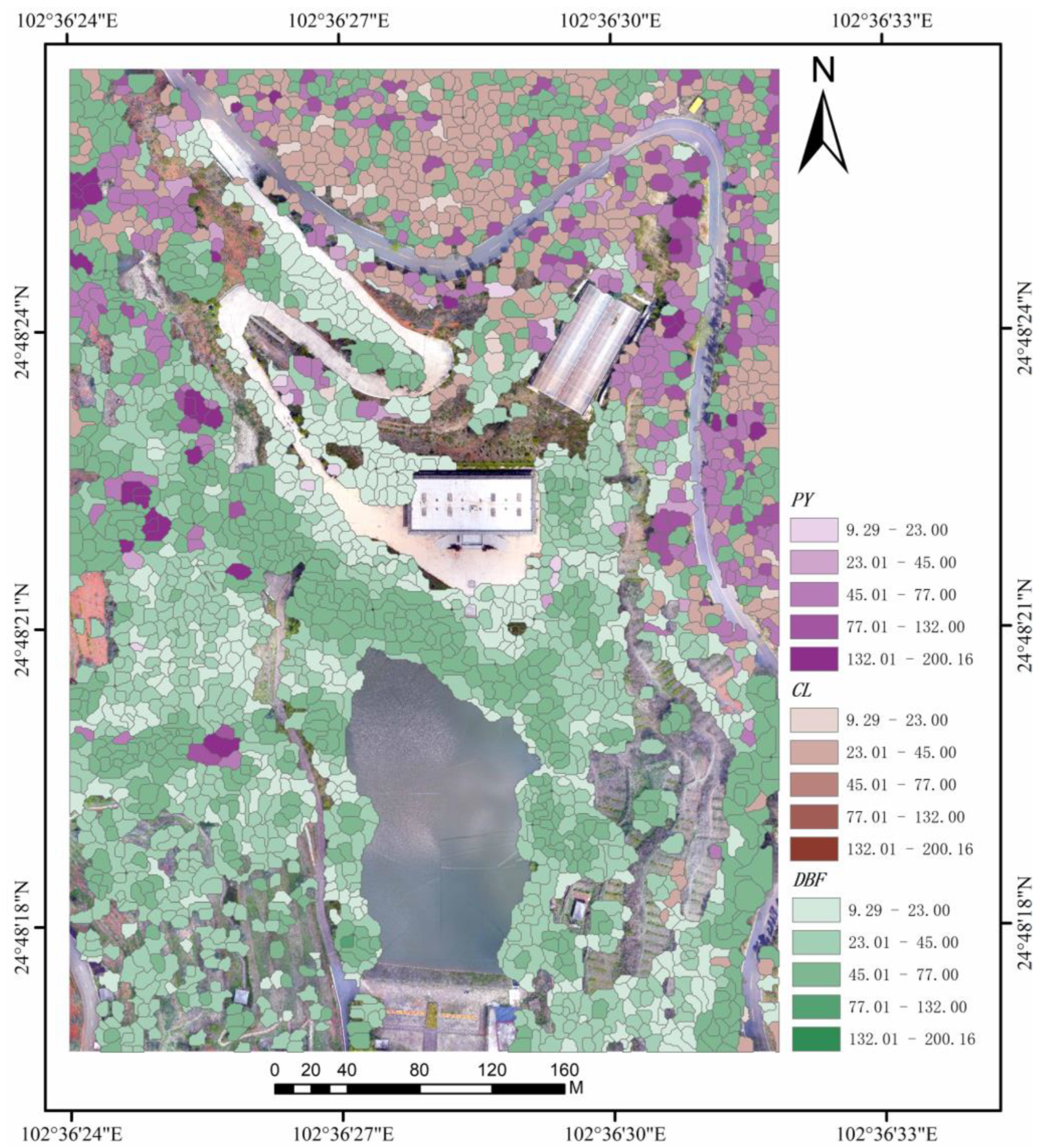
- A total of 2490 individual trees were segmented in the study area, which included 388 strains of Cupressus lusitanica, 343 strains of Pinus yunnanensis, and 1759 strains of Deciduous Broad-leaved Forest. The total biomass of the forest in the study area was 104,102.76 kg, including 12,399.61 kg of Cupressus lusitanica, 25,331.82 kg of Pinus yunnanensis, and 66,371.33 kg of Deciduous Broad-leaved Forest. The mean biomass of Pinus yunnanensis was the highest (73.85 kg) and its number of individuals with high biomasses was the largest.
- (3)
- From the estimation results of the two models, the random forest model with a poor learning ability showed better generalization ability in biomass estimation experiments with small samples and high dimensional data. Therefore, it is extremely necessary to collect more sample data when an estimation model with stronger learning ability is needed to improve the estimation accuracy.
Author Contributions
Funding
Institutional Review Board Statement
Informed Consent Statement
Data Availability Statement
Acknowledgments
Conflicts of Interest
References
- Latella, M.; Raimondo, T.; Belcore, E.; Salerno, L.; Camporeale, C. On the integration of LiDAR and field data for riparian biomass estimation. J. Environ. Manag. 2022, 322, 116046. [Google Scholar] [CrossRef]
- Qin, H.; Zhou, W.; Qian, Y.; Zhang, H.; Yao, Y. Estimating aboveground carbon stocks of urban trees by synergizing ICESat-2 LiDAR with GF-2 data. Urban For. Urban Green. 2022, 76, 127728. [Google Scholar] [CrossRef]
- Luther, J.; Fournier, R.; Piercey, D.; Guindon, L.; Hall, R. Biomass mapping using forest type and structure derived from Landsat TM imagery. Int. J. Appl. Earth Obs. Geoinform. 2006, 8, 173–187. [Google Scholar] [CrossRef]
- Hao, W.F.; Chen, C.; Liang, Z.; Ma, L. Research advances in vegetation biomass. J. Northwest A F Univ. Nat. Sci. Ed. 2008, 36, 175–182. [Google Scholar]
- Zhang, C.; Peng, D.-L.; Huang, G.-S.; Zeng, W.-S. Developing Aboveground Biomass Equations Both Compatible with Tree Volume Equations and Additive Systems for Single-Trees in Poplar Plantations in Jiangsu Province, China. Forests 2016, 7, 32. [Google Scholar] [CrossRef]
- Chakraborty, T.; Saha, S.; Reif, A. Biomass equations for European beech growing on dry sites. iFor. Biogeosci. For. 2016, 9, 751–757. [Google Scholar] [CrossRef]
- Li, H.; Li, C.; Zha, T.; Liu, J.; Jia, X.; Wang, X.; Chen, W.; He, G. Patterns of biomass allocation in an age-sequence of secondary Pinus bungeana forests in China. For. Chron. 2014, 90, 169–176. [Google Scholar] [CrossRef]
- Huang, G.; Li, Y. Phenological transition dictates the seasonal dynamics of ecosystem carbon exchange in a desert steppe. J. Veg. Sci. 2014, 26, 337–347. [Google Scholar] [CrossRef]
- Cao, L.; Liu, H.; Fu, X.; Zhang, Z.; Shen, X.; Ruan, H. Comparison of UAV LiDAR and Digital Aerial Photogrammetry Point Clouds for Estimating Forest Structural Attributes in Subtropical Planted Forests. Forests 2019, 10, 145. [Google Scholar] [CrossRef]
- Chen, S.; McDermid, G.J.; Castilla, G.; Linke, J. Measuring Vegetation Height in Linear Disturbances in the Boreal Forest with UAV Photogrammetry. Remote Sens. 2017, 9, 1257. [Google Scholar] [CrossRef]
- Hasan, U.; Sawut, M.; Chen, S. Estimating the Leaf Area Index of Winter Wheat Based on Unmanned Aerial Vehicle RGB-Image Parameters. Sustainability 2019, 11, 6829. [Google Scholar] [CrossRef]
- Wang, X.; Wang, Y.; Zhou, C.; Yin, L.; Feng, X. Urban forest monitoring based on multiple features at the single tree scale by UAV. Urban For. Urban Green. 2021, 58, 126958. [Google Scholar] [CrossRef]
- Niu, Y.; Zhang, L.; Zhang, H.; Han, W.; Peng, X. Estimating Above-Ground Biomass of Maize Using Features Derived from UAV-Based RGB Imagery. Remote Sens. 2019, 11, 1261. [Google Scholar] [CrossRef]
- Zheng, H.B.; Cheng, T.; Zhou, M.; Li, D.; Yao, X.; Tian, Y.C.; Cao, W.X.; Zhu, Y. Improved estimation of rice aboveground biomass combining textural and spectral analysis of UAV imagery. Precis. Agric. 2019, 20, 611–629. [Google Scholar] [CrossRef]
- Wang, Z.; Ma, Y.; Chen, P.; Yang, Y.; Fu, H.; Yang, F.; Raza, M.; Guo, C.; Shu, C.; Sun, Y.; et al. Estimation of Rice Aboveground Biomass by Combining Canopy Spectral Reflectance and Un-manned Aerial Vehicle-Based Red Green Blue Imagery Data. Front. Plant Sci. 2022, 13, 903643. [Google Scholar] [CrossRef]
- Liu, S.; Yang, G.; Jing, H.; Feng, H.; Li, H.; Chen, P.; Yang, W. Retrieval of winter wheat nitrogen content based on UAV digital image. Trans. Chin. Soc. Agric. Engin. 2019, 35, 75–85. [Google Scholar]
- Liu, Y.; Huang, J.; Sun, Q.; Feng, H. Estimation of plant height and above ground biomass of potato based on UAV digital image. Natl. Remote Sens. Bull. 2021, 25, 2004–2014. [Google Scholar]
- Che, Y.; Wang, Q.; Li, S.; Li, B.; Ma, Y. Monitoring of maize phenotypic traits using super-resolution reconstruction and multimodal data fusion. Trans. Chin. Soc. Agric. Eng. 2021, 37, 169–178. [Google Scholar]
- Wang, L.; Zheng, N.; Chen, H.; Li, D.; Wu, M.; Zhao, W. Remote estimation of canopy height and aboveground biomass of maize using high-resolution stereo images from a low-cost unmanned aerial vehicle system. Ecol. Indic. 2016, 67, 637–648. [Google Scholar] [CrossRef]
- Li, B.; Wu, X.; Zhang, L.; Han, J.; Bian, C.; Li, G.; Liu, J.; Jin, L. Above-ground biomass estimation and yield prediction in potato by using UAV-based RGB and hyperspectral imaging. ISPRS J. Photogramm. Remote Sens. 2020, 162, 161–172. [Google Scholar] [CrossRef]
- Liu, Y.; Liu, S.; Li, J.; Guo, X.; Wang, S.; Lu, J. Estimating biomass of winter oilseed rape using vegetation indices and texture metrics derived from UAV multispectral images. Comput. Electron. Agric. 2019, 166, 105026. [Google Scholar] [CrossRef]
- Li, C.; Yu, Z.; Wang, S.; Wu, F.; Wen, K.; Qi, J.; Huang, H. Crown Structure Metrics to Generalize Aboveground Biomass Estimation Model Using Airborne Laser Scanning Data in National Park of Hainan Tropical Rainforest, China. Forests 2022, 13, 1142. [Google Scholar] [CrossRef]
- Liu, F.; Tan, C.; Lei, P.-F. Estimating individual tree aboveground biomass of the mid-subtropical forest using air-borne LiDAR technology. J. Appl. Ecol. 2014, 25, 3229–3236. [Google Scholar]
- Rodríguez-Vivancos, A.; Manzanera, J.A.; Martín-Fernández, S.; García-Cimarras, A.; García-Abril, A. Analysis of structure from motion and airborne laser scanning features for the evaluation of forest structure. Eur. J. For. Res. 2022, 141, 447–465. [Google Scholar] [CrossRef]
- Tao, S.; Guo, Q.; Li, L.; Xue, B.; Kelly, M.; Li, W.; Xu, G.; Su, Y. Airborne Lidar-derived volume metrics for aboveground biomass estimation: A com-parative assessment for conifer stands. Agric. For. Meteorol. 2014, 198, 24–32. [Google Scholar] [CrossRef]
- Ullah, S.; Dees, M.; Datta, P.; Adler, P.; Koch, B. Comparing Airborne Laser Scanning, and Image-Based Point Clouds by Semi-Global Matching and Enhanced Automatic Terrain Extraction to Estimate Forest Timber Volume. Forests 2017, 8, 215. [Google Scholar] [CrossRef]
- Gao, L.; Zhang, X. Above-Ground Biomass Estimation of Plantation with Complex Forest Stand Structure Using Multiple Features from Airborne Laser Scanning Point Cloud Data. Forests 2021, 12, 1713. [Google Scholar] [CrossRef]
- Meng, Y.; Gou, R.; Bai, J.; Moreno-Mateos, D.; Davis, C.C.; Wan, L.; Song, S.; Zhang, H.; Zhu, X.; Lin, G. Spatial patterns and driving factors of carbon stocks in mangrove forests on Hainan Island, China. Glob. Ecol. Biogeogr. 2022, 31, 1692–1706. [Google Scholar] [CrossRef]
- Wang, J.; Xiao, X.; Bajgain, R.; Starks, P.; Steiner, J.; Doughty, R.B.; Chang, Q. Estimating leaf area index and aboveground biomass of grazing pastures using Sentinel-1, Sentinel-2 and Landsat images. ISPRS J. Photogramm. Remote Sens. 2019, 154, 189–201. [Google Scholar] [CrossRef]
- Liu, Y.; Zhuang, Y.; Ji, B.; Zhang, G.; Rong, L.; Teng, G.; Wang, C. Prediction of laying hen house odor concentrations using machine learning models based on small sample data. Comput. Electron. Agric. 2022, 195, 106849. [Google Scholar] [CrossRef]
- Hoover, C.M.; Ducey, M.J.; Colter, R.A.; Yamasaki, M. Evaluation of alternative approaches for landscape-scale biomass es-timation in a mixed-species northern forest. For. Ecol. Manag. 2018, 409, 552–563. [Google Scholar] [CrossRef]
- Asner, G.P.; Mascaro, J.; Muller-Landau, H.; Vieilledent, G.; Vaudry, R.; Rasamoelina, M.; Hall, J.S.; van Breugel, M. A universal airborne LiDAR approach for tropical forest carbon mapping. Oecologia 2011, 168, 1147–1160. [Google Scholar] [CrossRef]
- Zhang, Y.; Xia, C.; Zhang, X.; Cheng, X.; Feng, G.; Wang, Y.; Gao, Q. Estimating the maize biomass by crop height and narrowband vegetation indices derived from UAV-based hyperspectral images. Ecol. Indic. 2021, 129, 107985. [Google Scholar] [CrossRef]
- Pan, P.; Li, R.; Xiang, C.; Zhu, Z.; Yin, X. Biomass and Productivity Of Cupressus Lusitanica Plantation. Resour. Environ. Yangtze Val. 2002, 11, 133–136. [Google Scholar]
- Zhou, G.; Yin, G.; Tang, X.; Wen, D.; Liu, C.; Kuang, Y.; Wang, W. Biomass Equation and Evaluation of Dominant Tree Species in China, Carbon Stocking-Biomass Equation of Forest Ecosystems in China; Science Press: Beijing, China, 2018; pp. 40–80. [Google Scholar]
- Hendrawan, Y.; Fauzi, M.R.; Khoirunnisa, N.S.; Andreane, M.; Hartianti, P.O.; Halim, T.D.; Umam, C. Development of colour co-occurrence matrix (CCM) texture analysis for biosensing. IOP Conf. Ser. Earth Environ. Sci. 2019, 230, 012022. [Google Scholar] [CrossRef]
- Jin, L.; Li, Y. Analysis and realization of several correlation coefficients in R language. J. Stat. Inf. 2019, 34, 3–11. [Google Scholar]
- Yu, H.; Xie, S.; Guo, L.; Liu, P.; Zhang, P. Extremely Randomized Trees Estimation of Soil Heavy Metal Content by Fusing Spectra and Spatial Features. Trans. Chin. Soc. Agric. Mach. 2022, 53, 231–239. [Google Scholar]
- Chen, T.; Guestrin, C. XGBoost: A Scalable Tree Boosting System. CoRR 2016, 1603, 02754. [Google Scholar]
- Tian, Y.; Huang, H.; Zhou, G.; Zhang, Q.; Tao, J.; Zhang, Y.; Lin, J. Aboveground mangrove biomass estimation in Beibu Gulf using machine learning and UAV remote sensing. Sci. Total Environ. 2021, 781, 146816. [Google Scholar] [CrossRef]
- Liang, Y.; Kou, W.; Lai, H.; Wang, J.; Wang, Q.; Xu, W.; Wang, H.; Lu, N. Improved estimation of aboveground biomass in rubber plantations by fusing spectral and textural information from UAV-based RGB imagery. Ecol. Indic. 2022, 142, 109286. [Google Scholar] [CrossRef]
- David, R.M.; Rosser, N.J.; Donoghue, D.N. Improving above ground biomass estimates of Southern Africa dryland forests by combining Sentinel-1 SAR and Sentinel-2 multispectral imagery. Remote Sens. Environ. 2022, 282, 113232. [Google Scholar] [CrossRef]
- Zhou, Z. Feature Selection and Sparse Learning. In Machine Learning; Tsinghua University Press: Beijing, China, 2016; pp. 247–252. [Google Scholar]
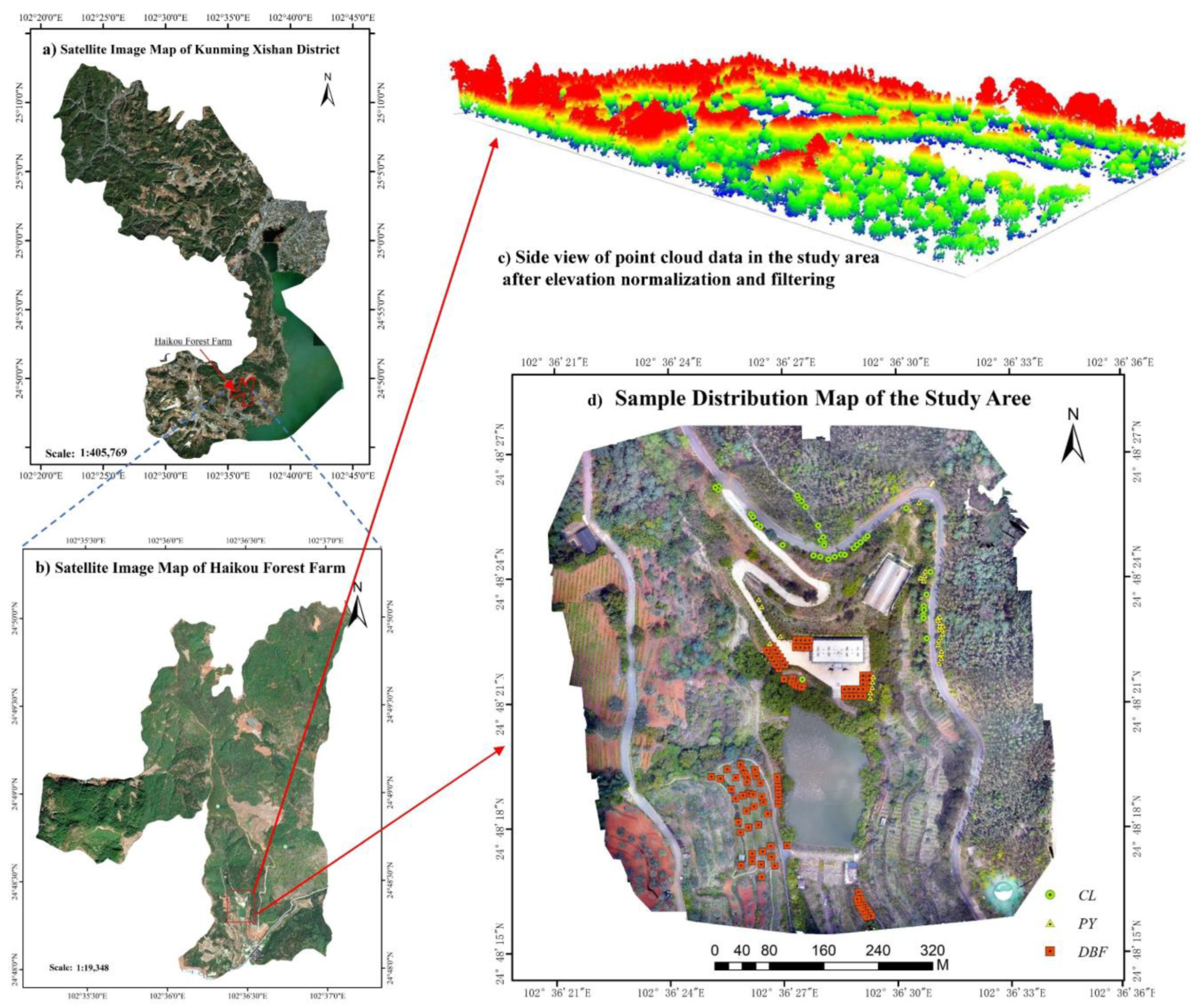



| Species | CL | PY | DBF | Total |
|---|---|---|---|---|
| Quantity | 36 | 31 | 107 | 174 |
| Species | Class | Equation | R2 | Reference |
|---|---|---|---|---|
| Cupressus lusitanica | Trunk | W = 38.57447×(D2H)0.88545 | 0.99 | [34] |
| Branch | W = 1.42899×(D2H)1.20845 | 0.98 | ||
| Leaf | W = 6.00855×(D2H)0.99494 | 0.99 | ||
| Root | W = 4.23742×(D2H)0.93532 | 0.99 | ||
| Pinus yunnanensis | Trunk | W = 0.009×(D2H)1.044 | 0.98 | [35] |
| Branch | W = 0.0008×(D2H)1.151 | 0.92 | ||
| Leaf | W = 0.006×(D2H)0.853 | 0.98 | ||
| Root | W = 0.009×(D2H)0.971 | 0.99 | ||
| Deciduous Broad-leaved Forest | Trunk | W = 0.0263×(D2H)0.9695 | 0.98 | [35] |
| Branch | W = 0.0232×(D2H)0.8055 | 0.97 | ||
| Leaf | W = 0.0075×(D2H)0.8015 | 0.96 | ||
| Root | W = 0.0381×(D2H)0.762 | 0.94 |
| Name | Parameters |
|---|---|
| AA450 airborne lidar sensor | Scanning frequency: 240,000 points/s (single echo), 720,000 points/s (triple echo); maximum range: 450 m; field angle: 70.4°(Horizontal) × 4.5°(Vertical) |
| Zenmuse P1 camera | Focal length: 24 mm; CCD size: 35.9 × 24 mm; Effective pixels: 45 million |
| Specie | CL | PY | DBF | Total |
|---|---|---|---|---|
| Quantity | 388 | 343 | 1759 | 2490 |
| Variable Name | Abbreviation | Variable Description | Reference |
|---|---|---|---|
| Red band | R | R = R | — |
| Green band | G | G = G | — |
| Blue band | B | B = B | — |
| Normalized red band | r | r = R/(R + G + B) | [14] |
| Normalized green band | g | g = G/(R + G + B) | [14] |
| Normalized blue band | b | b = B/(R + G + B) | [14] |
| Red–green ratio index | RGRI | RGRI = r/g | [14] |
| Green–blue ratio index | GBRI | GBRI = g/b | [14] |
| Red–blue ratio index | RBRI | RBVI = r/b | [14] |
| Red–blue difference index | RBDI | RBDI = r − b | [14] |
| Red–blue add index | RBAI | RBAI = r + b | [14] |
| Green–blue difference index | GBDI | GBDI = g − b | [14] |
| Red–blue vegetation index | RBVI | RBVI = (r − b)/(r + b) | [14] |
| Modified red–green–blue vegetation index | MRGBVI | MRGBVI = (r − b − g)/(r + g) | [14] |
| Modified green–red vegetation index | MGRVI | MGRVI = (g2 − r2)/(g2 + r2) | [14] |
| Red–green–blue vegetation index | RGBVI | RGBVI = (g2 − b × r)/(g2 + b × r) | [14] |
| Green–red vegetation index | GRVI | GRVI = (g − r)/(g + r) | [14] |
| Green leaf add index | GLA | GLA = (2 × g − r + b)/(2 × g + r + b) | [14] |
| Green leaf index | GLI | GLI = (2 × g − r − b)/(2 × g + r + b) | [14] |
| Excess red index | ExR | ExR = 1.4 × r − g | [14] |
| Excess green index | ExG | ExG = 2 × g − r − b | [14] |
| Excess green minus excess red index | ExGR | ExGR = ExG-1.4 × r − g | [14] |
| Color index of vegetation | CIVE | CIVE = 0.441 × r − 0.881 × g + 0.3856 × b + 18.78745 | [14] |
| Vegetation atmospheric resistance index | VARI | VARI = (g − r)/(g + r − b) | [14] |
| Warbeck index | WI | WI = (g − b)/(r − g) | [14] |
| Normalized difference index | NDI | NDI = (r − g)/(r + g + 0.01) | [15] |
| Normalized green–blue difference index | NGBVI | NGBDI = (g − b)/(g + b) | [15] |
| Vegetation index | VEG | VEG = g/(ra × b1−a); (a = 0.667) | [16] |
| Variable Name | Abbreviation | Variable Description | Reference |
|---|---|---|---|
| Mean | Mean | [36] | |
| Variance | Var | ||
| Homogeneity | Homo | ||
| Contrast | Con | ||
| Dissimilarity | Dis | ||
| Entropy | Ent | ||
| ASM | ASM | ||
| Correlation | Cor |
| Variable Name | Abbreviation | Quantity | Variable Description |
|---|---|---|---|
| Average absolute deviation | E-ADD | 1 | |
| Canopy relief rate | E-CRR | 1 | |
| Accumulate height percentiles | E-AIH | 15 | (X = 1,5,10,20,25,30,40,50,60,70,75,80,90,95,99) |
| Interquartile range of accumulate height percentile | E-AIH_IQ | 1 | |
| Variable coefficient | E-CV | 1 | |
| Kurtosis | E-Kurtosis | 1 | |
| Median of median absolute deviation | E-Mad median | 1 | The median absolute deviation of the median height value at all points in the region. |
| Maximum, minimum, mean, median, skewness, standard deviation, and variance | E-max, E-min, E-mean, E-median, E-skewness, E-stan, and E-var | 7 | The maximum, minimum, mean, median, skewness, standard deviation, and variance of all point heights in the region. |
| Quadratic power mean | E-SMS | 1 | |
| The mean to the third power | E-CMC | 1 | |
| Percentile of height | E-P | 15 | (X = 1,5,10,20,25,30,40,50,60,70,75,80,90,95,99) |
| Interquartile range of Percentile of height | E-PIQ | 1 |
| Variable Name | Abbreviation | Quantity | Variable Description |
|---|---|---|---|
| Mean absolute deviation | I-ADD | 1 | |
| Accumulate intensity percentiles | I-AII | 15 | (X = 1,5,10,20,25,30,40,50,60,70,75,80,90,95,99) |
| Variable coefficient | I-CV | 1 | |
| Kurtosis | I-Kurtosis | 1 | |
| Median of median absolute deviation | I-Mad median | 1 | The median absolute deviation of the median intensity value at all points in the region. |
| Maximum, minimum, mean, median, skewness, standard deviation, and variance | I-max, I-min, I-mean, I-median, I-skewness, I-stan, and I-var | 7 | The maximum, minimum, mean, median, skewness, standard deviation, and variance of intensity values of all points in the region. |
| Percentile of intensity | I-P | 15 | (X = 1, 5, 10, 20, 25, 30, 40, 50, 60, 70, 75, 80, 90, 95, and 99) |
| Interquartile range of percentile of intensity | I-PIQ | 1 |
| Variable Name | Abbreviation | Quantity | Variable Description |
|---|---|---|---|
| Density variable | D-M | 10 | In the region, the point cloud data are divided into ten equal height slices from low to high and the proportion of echo numbers in each layer is the corresponding density variable. |
| Canopy cover | CC | 1 | (nveg is the number of vegetation points, ntotal is the total number of points) |
| Leaf area index | LAI | 1 | (ang is the average scan Angle, GF is the gap rate, and k is the extinction coefficient) |
| Gap Fraction | GF | 1 | (nground is the number of ground points whose height is lower than the height threshold and n is the total number of points) |
| Variable Name | Abbreviation | Variable Description |
|---|---|---|
| Elevation | H | H = H |
| Slope | Slope | slope = slope |
| Aspect | Aspect | aspect = aspect |
| Slope Length | SL | |
| Slope Variability | SOS | SOS = slope of slope |
| Aspect Variability | SOA | SOA = slope of aspect |
| Terrain fluctuates degree | TFD | TFD = maxDEM − minDEM (Neighborhood range = 12) |
| Terrain Roughness | TR | |
| Crown Diameter | CD | The average diameter of the projected region of crown amplitude. |
| Tree Height | TreeH | The height difference between the top of the tree and the ground. |
| Crown Area | CA | The area of the projected region of crown amplitude |
| Crown Volume | CV | The volume of the canopy of a tree. |
| Class | Number | Minimum (kg) | Maximum (kg) | Mean (kg) | Variance (kg) |
|---|---|---|---|---|---|
| CL | 36 | 5.086 | 81.560 | 26.597 | 19.735 |
| PY | 31 | 2.552 | 275.846 | 63.785 | 64.533 |
| DBF | 107 | 3.652 | 98.689 | 28.753 | 17.735 |
| Tree Species | Quantity | Characteristics of Abbreviation |
|---|---|---|
| CL | 56 | R,G,B,r,g,RGRI,GBRI,VEG,0-Mean,0-Dis,45-Mean,45-Dis,90-Mean,90-Var,90-Dis,135-Mean,CanopyCover,LAI,E-AAD,E-CRR,E-AIH1st,E-AIHIQ,E-CV,E-PIQ,E-Kurtosis,E-Madmedian,E-Min,E-Skewness,D-M0,D-M1,D-M2,D-M3,D-M4,D-M5,D-M6,D-M7,D-M8,D-M9,I-AAD,I-CV,I-AII90th,I-Kurtosis,I-Madmedian,I-Max,I-Min,I-Skewness,I-PIQ,TreeHeight,C-Diameter,C-Volume,H,Slope,Aspect,Slopelength,SOS,SOA |
| PY | 59 | R,G,B,r,g,b,RGRI,GBRI,VARI,VEG,0-Mean,0-Dis,45-Mean,45-Dis,45-Ent,45-ASM,45-Cor,90-Var,90-Dis,135-Mean,CanopyCover,GapFraction,LAI,E-AAD,E-CRR,E-AIHIQ,E-CV,E-Kurtosis,D-M0,D-M1,D-M2,D-M3,D-M4,D-M5,D-M6,D-M7,D-M8,D-M9,I-AAD,I-CV,I-AII1st,I-AII99th,I-Kurtosis,I-Madmedian,I-Max,I-Min,I-Skewness,I-Variance,I-P1st,I-PIQ,TreeHeight,C-Diameter,C-Volume,H,Slope,Aspect,SlopeL,SOS,SOA |
| DBF | 50 | R,G,B,RGRI,GBRI,ExGR,0-Mean,0-Dis,45-Mean,90-Dis,135-Mean,CanopyCover,GapFraction,LAI,E-CRR,E-AIH1st,E-CV,E-Kurtosis,E-M,E-Skewness,D-M0,D-M1,D-M2,D-M3,D-M4,D-M5,D-M6,D-M7,D-M8,D-M9,I-AAD,I-CV,I-AII1st,I-AII99th,I-Kurtosis,I-Madmedian,I-Max,I-Min,I-Skewness,I-P1st,I-P10th,I-PIQ,TreeHeight,C-Diameter,H,Slope,Aspect,Slopelength,SOS,SOA |
| Tree Species | Quantity | Characteristics of Abbreviation |
|---|---|---|
| CL | 70 | r,RBDI,GBDI,RBVI,RGBDVI,WI,NGBDI,90-Dis,90-Ent,90-ASM,90-Cor,GapFraction,E-AAD,E-AIH70th,E-AIH75th,E-AIH80th,E-AIH90th,E-AIH95th,E-AIH99th,E-AIHIQ,E-CMC,E-CV,E-PIQ,E-Madmedian,E-Max,E-P40th,E-P50th,E-P60th,E-P70th,E-P75th,E-P80th,E-P90th,E-P95th,E-P99th,E-Skewness,E-SMS,E-Stddev,E-variance,D-M0,D-M1,D-M2,D-M3,D-M4,D-M5,D-M6,I-ALL1st,I-ALL5th,I-ALL10th,I-ALL20th,I-ALL25th,I-ALL30th,I-ALL40th,I-Max,I-Mean,I-Median,I-P1st,I-P8th,I-P9th,I-P10th,I-P11th,I-P12th,I-P13th,TreeHeight,C-diameter,C-area,C-Volume,Slope,Aspect,QFD,Groughness |
| PY | 87 | R,G,B,GBRI,RBRI,MRBVI,RBVI,GLA,ExGR,VARI,VEG,0-Mean,0-Var,0-Homo,0-Can,0-Dis,0-Ent,0-ASM,0-Cor,45-Mean,45-Var,45-Homo,135-Dis,135-Ent,135-ASM,135-Cor,CanopyCover,GapFraction,E-AAD,E-CRR,E-AIH1st,E-AIH5th,E-AIH10th,E-AIH20th,E-AIH25th,E-AIH30th,E-AIH40th,E-AIH50th,E-AIH60th,E-AIH70th,E-AIH75th,E-AIH80th,E-AIH90th,E-AIH95th,E-AIH99th,E-AIHIQ,E-CMC,E-PIQ,E-Kurtosis,E-Madmedian,E-Max,E-Min,E-Mean,E-Median,E-P1st,E-P5th,E-P10th,E-P20th,E-P25th,E-P30th,E-P40th,E-P50th,E-P60th,E-P70th,E-P75th,E-P80th,E-P90th,E-P95th,E-P99th,E-SMS,E-Stddev,E-variance,D-M6,D-M7,D-M8,D-M9,I-CV,TreeHeight,C-diameter,C-area,C-Volume,H,Slope,Aspect,SOS,QFD,Groughness |
| DBF | 77 | b,GBRI,RBRI,MRBVI,RBVI,GLA,ExGR,VARI,VEG,45-Mean,45-Var,45-Homo,45-Can,135-Mean,135-Var,135-Homo,135-Can,CanopyCover,GapFraction,E-AAD,E-CRR,E-AIH1st,E-AIH5th,E-AIH10th,E-AIH20th,E-AIH25th,E-AIH30th,E-AIH40th,E-AIH50th,E-AIH60th,E-AIH70th,E-AIH75th,E-AIH80th,E-AIH90th,E-AIH95th,E-AIH99th,E-AIHIQ,E-CMC,E-CV,E-PIQ,E-Madmedian,E-Max,E-Mean,E-Median,E-P1st,E-P5th,E-P10th,E-P20th,E-P25th,E-P30th,E-P40th,E-P50th,E-P60th,E-P70th,E-P75th,E-P80th,E-P90th,E-P95th,E-P99th,E-SMS,E-Stddev,E-variance,D-M6,D-M9,I-CV,I-ALL90th,I-Kurtosis,I-Max,I-Skewness,TreeHeight,C-diameter,C-area,C-Volume,Slope,SOS,QFD,Groughness |
| Tree Species | Quantity | Characteristics of Abbreviation |
|---|---|---|
| CL | 53 | G,B,b,GBRI,RBDI,GBDI,RBVI,RGBDVI,RGBVI,GLI,ExG,WI,NGBDI,0-Dis,0-ASM,45-Var,45-Dis,45-ASM,90-Can,135-Can,135-Ent,135-ASM,E-AAD,E-AIH99th,E-AIHIQ,E-CMC,E-CV,E-Kurtosis,E-Madmedian,E-P1st,E-Stddev,E-variance,D-M1,D-M3,D-M4,D-M5,D-M6,D-M7,D-M9,I-ALL10th,I-ALL90th,I-ALL95th,I-Kurtosis,I-Madmedian,I-Max,I-Min,I-P1st,I-P13th,I-P18th,I-PIQ,C-area,C-Volume,H |
| PY | 101 | R,G,r,RGRI,RBRI,RBDI,RGBDVI,MRBVI,ExGR,VARI,NGBDI,VEG,0-Var,0-Homo,0-Dis,0-Ent,0-ASM,0-Cor,45-Ent,45-Cor,90-Homo,135-Dis,135-Ent,135-ASM,135-Cor,E-AAD,E-CRR,E-AIH1st,E-AIH5th,E-AIH10th,E-AIH20th,E-AIH25th,E-AIH40th,E-AIH50th,E-AIH60th,E-AIH70th,E-AIH80th,E-AIH90th,E-AIH95th,E-AIH99th,E-AIHIQ,E-CMC,E-PIQ,E-Madmedian,E-Max,E-Mean,E-Median,E-P5th,E-P20th,E-P25th,E-P30th,E-P40th,E-P50th,E-P60th,E-P70th,E-P75th,E-P90th,E-P95th,E-P99th,E-SMS,E-variance,D-M1,D-M2,D-M4,D-M7,D-M9,I-AAD,I-ALL1st,I-ALL5th,I-ALL10th,I-ALL20th,I-ALL25th,I-ALL50th,I-ALL70th,I-ALL99th,I-Madmedian,I-Min,I-Skewness,I-Variance,I-P5th,I-P6th,I-P7th,I-P8th,I-P9th,I-P11th,I-P12th,I-P13th,I-P14th,I-P16th,I-P17th,I-P18th,I-PIQ,TreeHeight,C-diameter,C-area,C-Volume,H,SlopeL,SOS,SOA,QFD |
| DBF | 97 | g,b,RBRI,RBAI,GBDI,MRBVI,RGBVI,ExGR,0-Mean,0-Var,0-Homo,0-Can,0-Dis,45-Mean,45-Dis,45-Ent,45-ASM,45-Cor,90-Dis,90-Ent,90-ASM,135-Mean,135-Can,135-Dis,135-Ent,135-ASM,135-Cor,LAI,E-AAD,E-CRR,E-AIH1st,E-AIH10th,E-AIH20th,E-AIH25th,E-AIH30th,E-AIH40th,E-AIH50th,E-AIH60th,E-AIH70th,E-AIH75th,E-AIH80th,E-AIH90th,E-AIH95th,E-AIH99th,E-AIHIQ,E-CMC,E-PIQ,E-Madmedian,E-Max,E-Mean,E-Median,E-P1st,E-P5th,E-P10th,E-P20th,E-P25th,E-P30th,E-P40th,E-P50th,E-P60th,E-P70th,E-P75th,E-P80th,E-P90th,E-P95th,E-P99th,E-SMS,E-Stddev,E-variance,D-M0,D-M2,D-M5,D-M6,I-ALL1st,I-ALL25th,I-ALL60th,I-ALL80th,I-ALL90th,I-Max,I-Mean,I-Min,I-Skewness,I-P5th,I-P6th,I-P8th,I-P10th,I-P11th,I-P13th,I-P15th,I-P16th,I-PIQ,TreeHeight,C-diameter,C-area,C-Volume,H,SOA |
| Model Name | Parameters Range |
|---|---|
| RF | Number of decision trees (n_estimators): [50,300], Sampling interval: 20 Maximum depth of the model (max_depth): [3,10], Sampling interval: 2 Maximum number of input features in a single tree (max_features): [2,20], Sampling interval: 2 |
| XGBoost | Number of decision trees (n_estimators): [50,300], Sampling interval: 20 Maximum depth of the model (max_depth): [3,10], Sampling interval: 2 Learning rate of gradient descent (learning_rate): [0.01,0.3], Sampling interval: 0.01 |
| Species | Class | Number | Max Depth | Estimators | Max Features | RMSE of Train Set | R2 of Train Set | RMSE of Test Set | R2 of Test Set |
|---|---|---|---|---|---|---|---|---|---|
| CL | Image | 60 | 9 | 170 | 2 | 0.1157 | 0.8163 | 0.2061 | 0.1859 |
| Point cloud | 101 | 3 | 90 | 4 | 0.1150 | 0.8186 | 0.1315 | 0.6684 | |
| Image + Point cloud | 161 | 3 | 50 | 16 | 0.1127 | 0.8258 | 0.1334 | 0.6586 | |
| Image + Other | 72 | 9 | 130 | 14 | 0.1008 | 0.8606 | 0.1850 | 0.3440 | |
| Point cloud + Other | 113 | 9 | 110 | 6 | 0.0951 | 0.8760 | 0.1219 | 0.7152 | |
| ALL | 173 | 5 | 130 | 12 | 0.0999 | 0.8632 | 0.1209 | 0.7197 | |
| PY | Image | 60 | 9 | 50 | 2 | 0.0824 | 0.8679 | 0.2056 | 0.3479 |
| Point cloud | 101 | 5 | 90 | 18 | 0.0467 | 0.9576 | 0.1123 | 0.8055 | |
| Image + Point cloud | 161 | 9 | 50 | 14 | 0.0463 | 0.9583 | 0.1087 | 0.8176 | |
| Image + Other | 72 | 9 | 50 | 16 | 0.0643 | 0.9194 | 0.1748 | 0.5285 | |
| Point cloud + Other | 113 | 7 | 50 | 6 | 0.0463 | 0.9582 | 0.1119 | 0.8068 | |
| ALL | 173 | 9 | 50 | 18 | 0.0347 | 0.9766 | 0.1035 | 0.8347 | |
| DBF | Image | 60 | 5 | 50 | 12 | 0.0660 | 0.8803 | 0.1158 | 0.5622 |
| Point cloud | 101 | 9 | 90 | 12 | 0.0501 | 0.9309 | 0.1107 | 0.5996 | |
| Image + Point cloud | 161 | 5 | 50 | 8 | 0.0635 | 0.8890 | 0.1049 | 0.6406 | |
| Image + Other | 72 | 5 | 50 | 16 | 0.0645 | 0.8855 | 0.1034 | 0.6508 | |
| Point cloud + Other | 113 | 9 | 50 | 12 | 0.0574 | 0.9092 | 0.1146 | 0.5706 | |
| ALL | 173 | 9 | 110 | 16 | 0.0542 | 0.9193 | 0.1045 | 0.6429 |
| Species | Class | Number | Max Depth | Estimators | Max Features | RMSE of Train Set | R2 of Train Set | RMSE of Test Set | R2 of Test Set |
|---|---|---|---|---|---|---|---|---|---|
| CL | Image | 60 | 7 | 50 | 0.55 | 0.0003 | 1.0000 | 0.3062 | −0.7972 |
| Point cloud | 101 | 3 | 210 | 0.03 | 0.1183 | 0.8081 | 0.1429 | 0.6084 | |
| Image + Point cloud | 161 | 7 | 50 | 0.43 | 0.0003 | 1.0000 | 0.2030 | 0.2102 | |
| Image + Other | 72 | 3 | 50 | 0.53 | 0.0003 | 1.0000 | 0.1943 | 0.2766 | |
| Point cloud + Other | 113 | 3 | 50 | 0.13 | 0.1018 | 0.8580 | 0.1330 | 0.6611 | |
| ALL | 173 | 3 | 110 | 0.16 | 0.0021 | 0.9999 | 0.1175 | 0.5489 | |
| PY | Image | 60 | 3 | 50 | 0.47 | 0.0003 | 1.0000 | 0.2268 | 0.2070 |
| Point cloud | 101 | 3 | 50 | 0.57 | 0.0003 | 1.0000 | 0.2154 | 0.2845 | |
| Image + Point cloud | 161 | 3 | 90 | 0.21 | 0.0004 | 1.0000 | 0.1985 | 0.3923 | |
| Image + Other | 72 | 3 | 50 | 0.69 | 0.0002 | 1.0000 | 0.1320 | 0.7314 | |
| Point cloud + Other | 113 | 5 | 70 | 0.43 | 0.0002 | 1.0000 | 0.1982 | 0.3943 | |
| ALL | 173 | 5 | 70 | 0.43 | 0.0003 | 1.0000 | 0.1765 | 0.5195 | |
| DBF | Image | 60 | 5 | 90 | 0.25 | 0.0003 | 1.0000 | 0.1191 | 0.5363 |
| Point cloud | 101 | 7 | 50 | 0.69 | 0.0002 | 1.0000 | 0.1150 | 0.5680 | |
| Image + Point cloud | 161 | 7 | 70 | 0.35 | 0.0002 | 1.0000 | 0.1115 | 0.5936 | |
| Image + Other | 72 | 5 | 50 | 0.47 | 0.0003 | 1.0000 | 0.1122 | 0.5888 | |
| Point cloud + Other | 113 | 9 | 50 | 0.45 | 0.0002 | 1.0000 | 0.1091 | 0.6108 | |
| ALL | 173 | 3 | 50 | 0.47 | 0.0002 | 1.0000 | 0.1103 | 0.6025 |
| Species | Method | Number | Max Depth | Estimators | Max Features | RMSE of Train Set | R2 of Train Set | RMSE of Test Set | R2 of Test Set |
|---|---|---|---|---|---|---|---|---|---|
| CL | MA | 56 | 3 | 50 | 4 | 0.1005 | 0.8614 | 0.1248 | 0.7013 |
| PY | 59 | 7 | 50 | 18 | 0.0492 | 0.9528 | 0.1605 | 0.6029 | |
| DBF | 50 | 9 | 70 | 18 | 0.0565 | 0.9122 | 0.1023 | 0.6578 | |
| CL | CC | 70 | 7 | 150 | 8 | 0.0976 | 0.8695 | 0.1188 | 0.7296 |
| PY | 87 | 7 | 70 | 10 | 0.0518 | 0.9477 | 0.1058 | 0.8275 | |
| DBF | 77 | 9 | 270 | 18 | 0.0515 | 0.9272 | 0.1162 | 0.5589 | |
| CL | PI | 53 | 3 | 70 | 4 | 0.1225 | 0.7942 | 0.1176 | 0.7346 |
| PY | 101 | 9 | 50 | 16 | 0.0385 | 0.9712 | 0.0960 | 0.8578 | |
| DBF | 97 | 5 | 70 | 16 | 0.0584 | 0.9061 | 0.0986 | 0.6823 |
| Species | Method | Number | Max Depth | Estimators | Max Features | RMSE of Train Set | R2 of Train Set | RMSE of Test Set | R2 of Test Set |
|---|---|---|---|---|---|---|---|---|---|
| CL | MA | 56 | 3 | 90 | 0.07 | 0.1166 | 0.8137 | 0.1653 | 0.4763 |
| PY | 59 | 3 | 50 | 0.47 | 0.0003 | 1.0000 | 0.1532 | 0.6382 | |
| DBF | 50 | 5 | 50 | 0.63 | 0.0002 | 1.0000 | 0.1112 | 0.5960 | |
| CL | CC | 70 | 7 | 50 | 0.13 | 0.1022 | 0.8567 | 0.1694 | 0.4496 |
| PY | 87 | 3 | 70 | 0.43 | 0.0003 | 1.0000 | 0.1677 | 0.5664 | |
| DBF | 77 | 9 | 50 | 0.69 | 0.0002 | 1.0000 | 0.1018 | 0.6614 | |
| CL | PI | 53 | 3 | 70 | 0.39 | 0.0003 | 1.0000 | 0.1439 | 0.6032 |
| PY | 101 | 7 | 50 | 0.55 | 0.0003 | 1.0000 | 0.1319 | 0.7318 | |
| DBF | 97 | 3 | 50 | 0.55 | 0.0002 | 1.0000 | 0.1193 | 0.5349 |
| Species | Cupressus lusitanica | Pinus yunnanensis | Deciduous Broad-Leaved Forest | Total |
|---|---|---|---|---|
| Maximum (kg) | 44.96 | 200.16 | 77.06 | — |
| Minimum (kg) | 15.87 | 14.58 | 9.29 | — |
| Mean (kg) | 31.96 | 73.85 | 37.73 | — |
| Variance (kg) | 5.98 | 37.09 | 18.20 | — |
| Total (kg) | 12,399.61 | 25,331.82 | 66,371.33 | 104,102.76 |
Disclaimer/Publisher’s Note: The statements, opinions and data contained in all publications are solely those of the individual author(s) and contributor(s) and not of MDPI and/or the editor(s). MDPI and/or the editor(s) disclaim responsibility for any injury to people or property resulting from any ideas, methods, instructions or products referred to in the content. |
© 2023 by the authors. Licensee MDPI, Basel, Switzerland. This article is an open access article distributed under the terms and conditions of the Creative Commons Attribution (CC BY) license (https://creativecommons.org/licenses/by/4.0/).
Share and Cite
Yan, M.; Xia, Y.; Yang, X.; Wu, X.; Yang, M.; Wang, C.; Hou, Y.; Wang, D. Biomass Estimation of Subtropical Arboreal Forest at Single Tree Scale Based on Feature Fusion of Airborne LiDAR Data and Aerial Images. Sustainability 2023, 15, 1676. https://doi.org/10.3390/su15021676
Yan M, Xia Y, Yang X, Wu X, Yang M, Wang C, Hou Y, Wang D. Biomass Estimation of Subtropical Arboreal Forest at Single Tree Scale Based on Feature Fusion of Airborne LiDAR Data and Aerial Images. Sustainability. 2023; 15(2):1676. https://doi.org/10.3390/su15021676
Chicago/Turabian StyleYan, Min, Yonghua Xia, Xiangying Yang, Xuequn Wu, Minglong Yang, Chong Wang, Yunhua Hou, and Dandan Wang. 2023. "Biomass Estimation of Subtropical Arboreal Forest at Single Tree Scale Based on Feature Fusion of Airborne LiDAR Data and Aerial Images" Sustainability 15, no. 2: 1676. https://doi.org/10.3390/su15021676
APA StyleYan, M., Xia, Y., Yang, X., Wu, X., Yang, M., Wang, C., Hou, Y., & Wang, D. (2023). Biomass Estimation of Subtropical Arboreal Forest at Single Tree Scale Based on Feature Fusion of Airborne LiDAR Data and Aerial Images. Sustainability, 15(2), 1676. https://doi.org/10.3390/su15021676


