Evolutionary Game Mechanism of Governmental Cross-Regional Cooperation in AirPollution Management

Abstract

Intergovernmental collaboration is essential for regionally coordinated air pollution prevention and control. An evolutionary game model of local government behavior strategy selection taking into account the fixed cost of the local government, the total amount of network production factors, and the total amount of total network factors of production that can be moved is built based on the social capital theory in order to realize the cross-border collaborative control of regional air pollution. The issue of an intergovernmental cooperation framework for collaborative prevention and control of large-scale air pollution is addressed from the standpoint of the multi-stakeholder “benefit–cost” drive. Additionally, the major variables influencing the behavioral approach selection for intergovernmental cooperation are considered. The initial sensitivity of the evolution path of the local government behavioral strategy is also analyzed. The results of this study are: (1) The primary elements impacting intergovernmental cooperation on joint prevention and control of air pollution are fixed costs and fixed benefits, and reducing the fixed costs of such cooperation in an appropriate manner without compromising local governments’ pollution control can do so. (2) Under the assumption that local governments have fixed expenses, the total amount of network factors of production and total network factors of production that can be moved factors of production have a direct impact on intergovernmental cooperation. When local governments’ fixed costs are constant, they are more likely to choose the cooperative behavior option if the sum of their network production factors and total network factors of production that can be moved is higher. (3) The initial probability of cooperation among the three parties and the total amount of production factors have an impact on the system’s ESS when local governments in the area have equal total production factors. The study’s findings can offer theoretical justification for the “profit-driven” intergovernmental coordination of joint prevention and management of air pollution.

1. Introduction

The WHO (World Health Organization) figures show that 7 million individuals each year pass away as a result of air pollution (WHO, 2021) [1]. According to an article published on 18 May 2022 by India Express, the global death toll from air pollution alone would reach 6.67 million in 2019, with 1.67 million of those deaths occurring in India, the nation with the highest number of air pollution-related fatalities worldwide (Fuller et al., 2022) [2].

The International Organization for Standardization (ISO) defines air pollution, also known as atmospheric pollution, as the phenomenon where certain substances enter the atmosphere as a result of human activities or natural processes, present a sufficient concentration, reach a sufficient time, and thereby endanger human comfort, health, welfare, or the environment. When mankind first started using fire in the distant past, air pollution was already a problem (such as the burning of firewood, grassland, and forest fires, which will cause air pollution to varying degrees). However, following the Second World War, people in many industrialized countries began to understand that modern industry’s fast development, which began in the middle of the 18th century, was the primary cause of air pollution. The severity of the air pollution issue has increased (as

Table 1. Typical representatives of serious air pollution events in the 20th century.

Time	Locale	Event
1930	Mars Valley in Belgium	the smog event
1943	Los Angeles	the photochemical smog event
1952	London	the smog event
1961	Nihon City, Japan	the asthma event

). Due to the worsening environmental contamination in the late 1960s, some nations progressively began to launch environmental protection campaigns, pushing the government to take action to address the issue. The Human Environment Conference was held in 1972, and the Declaration of the United Nations Conference on Human Environment was adopted. The Declaration urges governments and citizens worldwide to work together to protect and enhance the human environment.

Governments have been compelled to pay attention to environmental protection and start controlling environmental pollution since the 1980s as a result of the growing demands of people in all countries for environmental protection. In numerous nations, investments in the prevention of and reduction in air pollution have expanded dramatically. Air pollution in some countries has been largely controlled, and the quality of the environment has significantly improved as a result of the successive formulation of pertinent air quality laws and air pollution control laws, the strengthening of strict environmental management, and the adoption of comprehensive prevention and control measures. Nevertheless, efforts must still be made to avoid and reduce air pollution on a worldwide scale. Incentives or policies to encourage cleaner industrial production, energy efficiency, and pollution reduction are increasingly being adopted by countries, according to the report of the United Nations Environment Programme’s 2021 Air Quality Action. More policies are also being developed to forbid the burning of solid waste. However, there is still a lot to be done. Only 31% of the countries have legislative frameworks in place to control or address cross-border air pollution, and 43% don’t even have a definition of air pollution in their laws. The majority of nations still don’t have a standardized framework for managing and monitoring air quality. The process of industrialization, economic power, smoke control regulations, and government resolve are all strongly correlated with the growth of China’s air pollution control business. China has steadily risen to the top of the worldwide air pollution prevention technology rankings during the past ten years. Applications for invention patents made up 34.1% of all applications in the previous ten years, with an average annual growth rate of about 30%. With 14.92% and 11.22% of the total, Japan and the United States came in second and third, respectively. The quantity change trend remained largely stable (UNEP, 2021) [3].

The natural law of atmospheric flow is violated by the territorial government based on administrative boundaries, and it is challenging to effectively address regional and complicated air pollution issues typified by ozone, fine particles, and acid rain. Additionally, the unilateral control impact will be further countered by the “pollution shelter” effect, resulting in low efficiency for provincial pollution management as a whole. Relevant academics have also noted the importance of intergovernmental cooperative governance in addressing the current, seriously escalating air pollution. Therefore, the primary axis of the development of the environmental protection system is the intergovernmental cooperation model of environmental governance. The central government has consistently encouraged horizontal cooperation between municipalities through policy planning with regard to the joint prevention and control of air pollution (The policies formulated are as

Table 2. The policies formulated for air pollution.

Organizations	Policies
East Asia Acid Deposition Monitoring Network	collected data in many fields, such as dust, water quality, soil and ecosystem, and has played an important role in assessing the acid deposition situation in East Asia and preventing further harm
China, Japan and South Korea in 2002	joint monitoring network of sandstorms built by realized data sharing and provided data support for cooperative control of sandstorms
In May 2010, General Office of the State Council	issued the Guiding Opinions On Promoting Joint Prevention and Joint Control Work Air On Air Pollution and Improving Regional Air Quality
In September 2013, the State Council	issued the Air Pollution Prevention and Control Action Plan
In July 2018, the State Council publicly	issued the Three-year Action Plan for Winning the Battle of Protecting the Blue Sky

). It is clear from the pertinent central government policies that regional intergovernmental cooperation has steadily replaced local control as the primary method of combating air pollution (General Office of the State Council, 2010; 2013) [4,5]. However, because air pollution is mobile, intergovernmental cooperation also encounters the following challenges. The government is prone to delegating governance duties to other governments out of self-interest because it is difficult to define the air pollution boundary in the air pollution problem. Second, local governments must consider production and economic structure issues when tackling air pollution. Achieving intergovernmental cooperation under factor changes is also the key to joint prevention and control of air pollution.

Air pollution is occurring more frequently as a result of the risk society, and it is challenging for a single local government department to handle the complex air pollution on its own. As a result, researchers have begun to focus on the collaborative management of air pollution in the field of emergency management. For this paper, the keywords “air pollution prevention and control,” “inter-governmental cooperation on air pollution,” and “cross-border management of air pollution” were used to search the Internet. In this study, the terms “air pollution prevention and control,” “inter-prefectural cooperation,” and “transboundary air pollution management” were used to search the Web and WOS databases. The following three aspects are the main focus of the pertinent studies. (1) Policies and effects of air pollution prevention and control. Some scholars have used parameters (Yang et al., 2019; Langbein et al., 2021) [6,7], the DID model (Xu et al., 2021; Meng et al., 2021; Bao et al., 2021) [8,9,10], the CGE models (Li et al., 2019; Zhang et al., 2020) [11,12], quasi-natural experiment (Xu et al., 2021; Jiang et al., 2021; Xu et al., 2020) [13,14,15], spatial panel model (Wu et al., 2019; Azimi et al., 2019; Zhang et al., 2020) [16,17,18], multilevel analysis (Zhang et al., 2020) [19], systems dynamics (Jia et al., 2019) [20], and Bayesian LSTM (Han et al., 2018) [21] to investigate whether these models can directly or indirectly improve air quality for air pollution control, and explore the factors and paths of policies affecting air quality. These previous studies have led to the following findings. Firstly, air pollution prevention and control policies can effectively reduce pollutant emissions. For developed areas (such as Beijing, Shanghai, and other places), the air improvement is more significant, indicating that the air pollution prevention and control policy has a certain dynamic control effect. Secondly, from a microscopic perspective, air pollution prevention and control policies can reduce the pollution emissions of enterprises. It promotes the reduction in corporate pollutants and greenhouse gas emissions, confirming the effectiveness of environmental policies. Finally, in terms of the spatial effect, the effectiveness of the environmental policy on air pollution control has improved in recent years. Furthermore, with the improvement of environmental regulation, the spatial spillover effect has been enhanced (Hao et al., 2021; Zhou et al., 2019) [22,23].

(2) Intergovernmental relations for air pollution control. In 2010, China proposed the establishment of a joint prevention and control mechanism for air pollution in key areas to jointly deal with pollution problems. In addition, scholars have discussed the necessity of government cooperation to control air pollution problems. Air pollution control is geographically limited, and air pollution has public goods attributes and negative externalities. Based on these characteristics, scholars have stated that joint actions across administrative regions must be carried out to fundamentally solve the regional air pollution problem (Xiao et al., 2020; Xu, 2018) [24,25]. With government coordination as the starting point, scholars investigated air pollution control in terms of responsibility-sharing mechanism (Ongaro, 2019; You, et al., 2020) [26,27], intergovernmental power division (Suo, 2021) [28], information communication mechanism (Jing et al., 2021; Li, 2020; Wu, 2020) [29,30,31]; policy coordination (Schwartz, 2019; Tian et al., 2020) [32,33] and institutional foundation and arrangements (Mao, 2021; Wen, 2020; Wei, 2018; Zhao, 2017) [34,35,36,37]. These studies have revealed that intergovernmental cooperation in air pollution control can effectively improve regional environmental quality.

(3) Cross-border spatial interaction of air pollution control. With the aim of making up for the shortcomings of the above study methods, spatial metrology-based methods were gradually applied (Kumar et al., 2009; Fernández-Avilés et al., 2012) [38,39]. In spatial metrology, most studies have focused on spatial spillover effects of air pollutant emissions and identified their main influencing factors (Feng et al., 2020; Vadrevu et al., 2020; Samoli et al., 2019; Kai et al., 2022) [40,41,42,43]. In addition, predictions of cross-border interactions of air pollution have also been made based on mathematical models such as the Markov chain (Alyousifi et al., 2020; Alyousifi et al., 2021) [44,45], artificial neural networks (Agarwal et al., 2020) [46], and deep learning (Hahnel et al. 2020) [47]. In summary, air pollution control has been a hot topic for experts and scholars in recent years, and various results have been achieved. However, in terms of the research content, it is mainly through mathematical models that the effects of air pollution control policies, inter-governmental cooperation, and transboundary interaction can be studied. Few studies have addressed local government information exchange and factor flow the air pollution control.

However, there is not much research that examines how to include the prevention and control of air pollution into an evolutionary game framework in terms of public governance. In actuality, it is difficult to prevent and control air pollution jointly due to a lack of regional resources. Resources are frequently distributed inequitably across municipal governments. Administrative divisions and fragmentation can unavoidably lead to collaboration and rivalry between regional and local governments.

The following are the goals of this study, which are based on the existing circumstances: (1) Examining the “benefit–cost” motive from the standpoint of local inter-county competition and cooperation in joint air pollution prevention and control. (2) Researching the key determinants of local intergovernmental cooperation. (3) Investigating the dynamic development of short-term intersectional cooperation. (4) Investigating the means by which local governments collaborate.

The following are the goals of this study, which are based on the existing circumstances: (1) This study can accomplish the aforementioned goals and show how behavioral strategy selection is competitive and cooperative for collaborative prevention and management of air pollution. Additionally, the governance of intergovernmental cooperation can be optimized, revealing the essence of cross-regional joint prevention and control from one perspective and aiding in the process of cross-regional joint prevention and control of air pollution while also enhancing the overall effectiveness of air pollution control.

In this essay, we looked at the root causes of the air pollution management dilemma in the area, the effects of internal and external dynamics on the growth of collaborative management, and recommendations to support the growth of collaborative air pollution management in the region. We can lessen the occurrence of abdicating duties and a lack of roles in collaborative air pollution management in order for local governments in China’s regions to better realize the management of air pollution. This will raise public confidence in local administrations while also enhancing China’s air quality.

The evolutionary game theory combines the analysis of game theory with the dynamic evolution process, which is a dynamic equilibrium. Nowadays, economists have also made remarkable achievements in using evolutionary game theory to analyze the factors affecting the formation of social habits, norms, institutions, or systems. Furthermore, their formation process has been explained (Wu et al., 2019) [16]. In recent years, domestic and foreign scholars’ research in evolutionary game theory and application has shown diversified characteristics. The evolutionary game model has been widely applied in product quality regulation (Liu et al., 2022) [48], environmental governance (Aghmashhadi et al., 2022) [49], collaborative innovation (Hosseini-Motlagh et al., 2022) [50], and so on.

As limited rational persons, local governments cooperate and compete in joint prevention and control of air pollution. Through the cognition of intergovernmental cooperation behavior rules. The behavioral strategies are constantly revised and improved to obtain “satisfactory” benefits. Therefore, under the theoretical framework of social capital, the local governments are assumed to be rational people, who are the interest subjects of their respective administrative regions. They pursue the maximization of the interests of their respective administrative regions for the purpose of their independent interest demands, and ultimately achieve the maximization of public interests in the cooperative network structure.

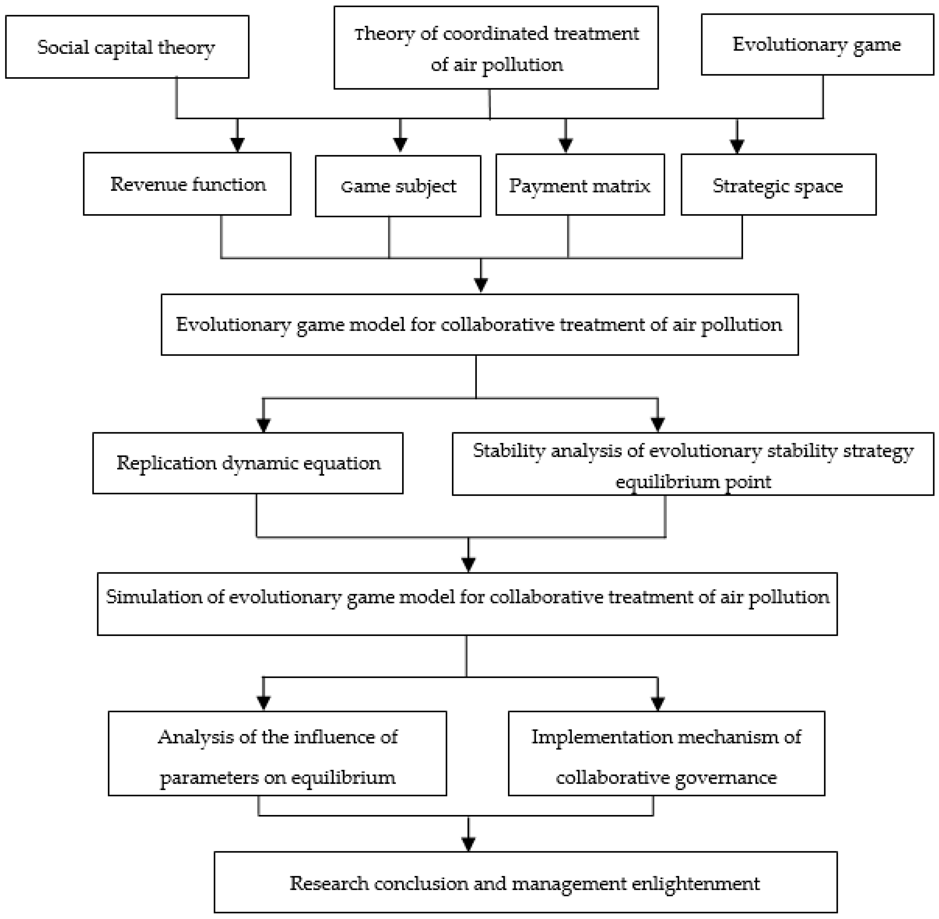
The remaining portions of this study are structured as follows. The model’s problem description and the pertinent parameter assumptions are covered in detail in Section 2. Section 3 analyzes the collaborative air pollution event management evolutionary game benefit matrix under the effect of internal factors and examines the individual government game scenarios through stability and equilibrium points. Through the use of simulations, Section 4 examines the developmental traits and shifting patterns of governmental actions in the process of cooperative air pollution management in the region. The study for this paper is summarized in Section 5, along with pertinent solutions and advice.

2. Problem Description and Parameter Setting

Pierre Bourdieu first formally put forth the idea of social capital in 1980 as a theoretical framework for elucidating the disparities between economic and social growth (Lamaison et al., 1986) [51]. Robert D. Putnam provided the classical definition of social capital as follows: “The characteristics of social organizations include social trust, social norms, and participation networks that promote cooperative behavior to improve social efficiency.” This is the framework for social capital that has been adopted by political and administrative circles (Putnam, 1994) [52].

The core component of social capital and the foundation for intergovernmental collaboration in the joint prevention and control of air pollution is social trust. Government cooperation is impossible without mutual confidence. The maximization of the public interest over individual interests is at the heart of collaborative prevention and control of air pollution. Mutual trust is necessary for interstate collaboration to continue smoothly. One of the key components of social capital and a crucial method of subject engagement is the social participation network, which serves as the conduit for communication and interaction between the social members. The formation of a network structure based on equality, trust, and cooperation is the core of intergovernmental cooperation on joint prevention and control of air pollution. In addition, it is also important to take joint action on air pollution control to maximize public interests.

The topics of cooperative air pollution control studied in this paper are limited to government subjects at the same level (the government plays an indispensable and significant role in the process of air pollution control, the government is the policy maker and the executive supervisor, the policies it promulgates and the actions it takes will be closely related to the effect of air pollution control). For example, when air pollution occurs in one region and has a direct or indirect impact on another region, different local governments in Jiangsu, Zhejiang, and Shanghai in the Yangtze River, which are members of the Cross-administrative region, work together through collaborative management to reduce the impact of air pollution and losses in order to create a win–win situation at the regional level.

Hypothesis 1 (H1).

There are three adjacent local governments in joint control of the prevention and control of air pollution, which are the main body of the evolutionary game, recorded as local government A, local government B, and local government C. The set of behavioral strategies for each local government is {Active cooperation, Passive treatment}. At a fixed time t, the proportion of local governments choosing cooperative behavioral strategies is $x,y,z$, and meets $0\le x\le 1$, $0\le y\le 1$, and $0\le z\le 1$.

Hypothesis 2 (H2).

There are some homogenous externalities between local governments in air pollution management, which indicates that one local government benefits from the pollution control of another local government. According to the social capital theory, regardless of whether actors employ cooperative methods, a specific proportion of returns (relative to the proportion of subjects actively cooperating with the three parties) can be acquired due to the liquidity of production inputs among regions (Dubos, 2017). Then, the gains of local government A, local government B, and local government C are assumed to be e₁ (x,y,z), e₂ (x,y,z), and $e_3(x,y,z)$, respectively, and $\frac{\partial e_i}{\partial x}>0$, $\frac{\partial e_i}{\partial y}>0$, $\frac{\partial e_i}{\partial z}>0$, $i=1,2,3$.

Hypothesis 3 (H3).

In air pollution control, if local governments adopt a behavioral strategy of active cooperation, they need to pay a certain cost, which is also related to the proportion of subjects with active cooperation between the three parties. Therefore, the cost of local government A is assumed to be $c_1(x,y,z)$, $\frac{\partial c_1}{\partial x}<0$, $\frac{\partial c_1}{\partial y}<0$, $\frac{\partial c_1}{\partial z}<0$. To simplify the model, assume $c_1(x,y,z)={\mu }_1-{\alpha }_{1}x-{\beta }_{1}y-{\gamma }_{1}z$. Similarly, for local government B, the cost of payment is $c_2(x,y,z)={\mu }_2-{\alpha }_{2}x-{\beta }_{2}y-{\gamma }_{2}z$, and the payment cost of local government C is $c_3(x,y,z)={\mu }_3-{\alpha }_{3}x-{\beta }_{3}y-{\gamma }_{3}z$. Among them, ${\mu }_1,{\mu }_2,{\mu }_3>0$ is a constant that represents the fixed cost for local government to choose the active cooperative behavioral strategy; ${\alpha }_i,{\beta }_i,{\gamma }_i>0,i=1,2,3$, represents the network production factors (capital, technology, and information) of local government organizations. The larger the value is, the higher the cooperation efficiency between governments will be, and the lower the cost they will pay for adopting the positive cooperation strategy.

The combined prevention and control of air pollution through intergovernmental cooperation is extremely important. Local governments can be “separated” from one another by the active participation of other local governments if they have high expectations for cross-border collaborative governance and high levels of recognition for it. This raises the cost of governing in the long run. The expense of combating air pollution can only be decreased by intergovernmental collaboration. Thus, the following is suggested for hypothesis 4:

Hypothesis 4 (H4).

When local governments adopt a non-cooperative strategy, they are subject to retaliation by local governments that choose active cooperation strategies (such as innovative technology and information sharing). The fixed opportunity cost that the uncooperative governments need to pay is constant η_i, i = 1, 2, 3. In addition, there are retaliatory losses from other local governments. The opportunity losses for local government A, local government B, and local government C to choose passive treatment strategies can be expressed as $r_1(y,z)={\eta }_1+{\tau }_{1}y+{\psi }_{1}z$, $r_2(x,z)={\eta }_2+{\tau }_{2}x+{\psi }_{2}z$, and $r_3(x,y)={\eta }_3+{\tau }_{3}x+{\psi }_{3}y$, respectively, where $\frac{\partial r_1}{\partial y}>0$, $\frac{\partial r_1}{\partial z}>0$, $\frac{\partial r_2}{\partial x}>0$, $\frac{\partial r_2}{\partial z}>0$, $\frac{\partial r_3}{\partial x}>0$, $\frac{\partial r_3}{\partial y}>0$. In particular, when only one local government chooses to cooperate actively, it retaliates against the other two local governments. When local government A chooses to cooperate, both local government B and local government C are subject to retribution from local government A. Then, the opportunity losses are $r_2(x)={\eta }_2+{\tau }_{2}x$ and $r_3(x)={\eta }_3+{\tau }_{3}x$. Similarly, $r_1(y)={\eta }_1+{\tau }_{1}y$, $r_3(y)={\eta }_3+{\psi }_{3}y$, $r_1(z)={\eta }_1+{\psi }_{1}z$, $r_2(z)={\eta }_2+{\psi }_{2}z$, where $\frac{\partial r_2}{\partial x}>0$, $\frac{\partial r_3}{\partial x}>0$, $\frac{\partial r_1}{\partial y}>0$, $\frac{\partial r_3}{\partial y}>0$, $\frac{\partial r_1}{\partial z}>0$, $\frac{\partial r_2}{\partial z}>0$ represents the flowable network production factors (funds, technology, and information) of local government organizations. The larger the value of the flowable network production the greater loss of passive treatment between governments and the greater expectation of adopting cooperative behavioral strategies.

Based on the above hypotheses, the earnings of the local government A choosing the active cooperative behavioral strategy is ${\Psi }_{11}=e_1(x,y,z)-c_1(x,y,z)$, and the earning of choosing the passive treatment behavioral strategy is ${\Psi }_{12}=e_1(x,y,z)-r_1(\otimes )$, where $\otimes$ represents whether the government chooses the active cooperative behavioral strategy. In the same way, the behavioral strategy benefits of local government B and local government C can be obtained. Based on the model assumptions and the description of related issues, the payment matrix of each local government can be obtained, as shown in

Table 3. Payment matrix of each local government.

Behavioral Policy Set	Local Government A	Local Government B	Local Government C
(1,1,1)	$e_1(x,y,z)-c_1(x,y,z)$	$e_2(x,y,z)-c_2(x,y,z)$	$e_3(x,y,z)-c_3(x,y,z)$
(1,1,0)	$e_1(x,y,z)-c_1(x,y,z)$	$e_2(x,y,z)-c_2(x,y,z)$	$e_3(x,y,z)-r_3(x,y)$
(1,0,1)	$e_1(x,y,z)-c_1(x,y,z)$	$e_2(x,y,z)-r_2(x,z)$	$e_3(x,y,z)-c_3(x,y,z)$
(1,0,0)	$e_1(x,y,z)-c_1(x,y,z)$	$e_2(x,y,z)-r_2(x)$	$e_3(x,y,z)-c_3(x,y,z)$
(0,1,1)	$e_1(x,y,z)-r_1(y,z)$	$e_2(x,y,z)-c_2(x,y,z)$	$e_3(x,y,z)-c_3(x,y,z)$
(0,1,0)	$e_1(x,y,z)-r_1(y)$	$e_2(x,y,z)-c_2(x,y,z)$	$e_3(x,y,z)-r_3(y)$
(0,0,1)	$e_1(x,y,z)-r_1(z)$	$e_2(x,y,z)-r_2(z)$	$e_3(x,y,z)-c_3(x,y,z)$
(0,0,0)	$e_1(x,y,z)-r_1(0)$	$e_2(x,y,z)-r_2(0)$	$e_3(x,y,z)-r_3(0)$

.

According to the evolutionary game theory and the above payment matrix, the replication dynamic equation of the local government A is:

$$\begin{array}{l}{G}_A(x,y,z)=x({\Psi }_{11}-{\overline{\Psi }}_1)=x(1-x)({\Psi }_{11}-{\Psi }_{12})\\ \hspace{1em}\hspace{1em}\hspace{1em}\hspace{1em}=x(1-x)[{\eta }_1-{\mu }_1+{\alpha }_{1}x+{\beta }_{1}y+{\gamma }_{1}z+{\tau }_1{y}^2+{\psi }_1{z}^2]\end{array}$$

(1)

Similarly, the replication dynamic equations for local governments B and C are:

$$\begin{array}{l}{G}_B(x,y,z)=y({\Psi }_{21}-{\overline{\Psi }}_2)=y(1-y)({\Psi }_{21}-{\Psi }_{22})\\ \hspace{1em}\hspace{1em}\hspace{1em}\hspace{1em}=y(1-y)[{\eta }_2-{\mu }_2+{\alpha }_{2}x+{\beta }_{2}y+{\gamma }_{2}z+{\tau }_2{x}^2+{\psi }_2{z}^2]\end{array}$$

(2)

$$\begin{array}{l}{G}_C(x,y,z)=z({\Psi }_{31}-{\overline{\Psi }}_3)=z(1-z)({\Psi }_{31}-{\Psi }_{32})\\ \hspace{1em}\hspace{1em}\hspace{1em}\hspace{1em}=z(1-z)[{\eta }_3-{\mu }_3+{\alpha }_{3}x+{\beta }_{3}y+{\gamma }_{3}z+{\tau }_3{x}^2+{\psi }_3{y}^2]\end{array}$$

(3)

Therefore, in the intergovernmental cooperation of joint prevention and governance of air pollution, the replication dynamic equations of various local government groups constitute the replication dynamic system of “benefit–cost” interests between networks:

$$\{\begin{array}{l}\frac{dx}{dt}=x(1-x)[{\eta }_1-{\mu }_1+{\alpha }_{1}x+{\beta }_{1}y+{\gamma }_{1}z+{\tau }_1{y}^2+{\psi }_1{z}^2]\\ \frac{dy}{dt}=y(1-y)[{\eta }_2-{\mu }_2+{\alpha }_{2}x+{\beta }_{2}y+{\gamma }_{2}z+{\tau }_2{x}^2+{\psi }_2{z}^2]\\ \frac{dz}{dt}=z(1-z)[{\eta }_3-{\mu }_3+{\alpha }_{3}x+{\beta }_{3}y+{\gamma }_{3}z+{\tau }_3{x}^2+{\psi }_3{y}^2]\end{array}$$

(4)

According to the scheme proposed by Friedman, the evolutionary stability strategy (ESS) of the system of differential equations can be obtained from the local stability analysis of the Jacobian matrix of this system. Therefore, the Jacobian matrix of the system can be obtained by replication dynamic Equation (4) as:

$$J=\left[\begin{array}{ccc}(1-2x){\Theta }_1& x(1-x)({\beta }_1+2{\tau }_{1}y)& x(1-x)({\gamma }_1+2{\psi }_{1}z)\\ y(1-y)({\alpha }_2+2{\tau }_{2}x)& (1-2y){\Theta }_2& y(1-y)({\gamma }_2+2{\psi }_{2}z)\\ z(1-z)({\alpha }_3+2{\tau }_{3}x)& z(1-z)({\beta }_3+2{\psi }_{3}y)& (1-2z){\Theta }_3\end{array}\right]$$

(5)

where

$$\begin{array}{l}{\Theta }_1={\eta }_1-{\mu }_1+{\alpha }_1+{\alpha }_{1}x+{\beta }_{1}y+{\gamma }_{1}z+{\tau }_1{y}^2+{\psi }_1{z}^2\\ {\Theta }_2={\eta }_2-{\mu }_2+{\beta }_2+{\alpha }_{2}x+{\beta }_{2}y+{\gamma }_{2}z+{\tau }_2{x}^2+{\psi }_2{z}^2\\ {\Theta }_3={\eta }_3-{\mu }_3+{\gamma }_3+{\alpha }_{3}x+{\beta }_{3}y+{\gamma }_{3}z+{\tau }_3{x}^2+{\psi }_3{y}^2\end{array}$$

In the replication dynamic system (4), when $\frac{dx}{dt}=\frac{dy}{dt}=\frac{dz}{dt}=0$, the local equilibrium points of (1,1,1,), (1,1,0), (1,0,1), (1,0,0), (0,1,1), (0,1,0), (0,0,1), and (0,0,0) can be obtained. The equilibrium point of the system is an unstable point when all the eigenvalues of the Jacobian matrix are larger than 0. The system’s equilibrium point is the gradual stable point where the eigenvalues are less than 0. The saddle point is where the system is in equilibrium whether the eigenvalues are positive or negative. For instance, for the pure strategy’s increasing stability in the local analysis method of the Jacobian matrix is used to study the Nash equilibrium point of the local equilibrium point (0,0,0), and the same method can be used to determine the gradual stability of other pure strategies. The Jacobian matrix of the local equilibrium point (0,0,0) is:

$$J_1=\left[\begin{array}{ccc}{\eta }_1-{\mu }_1+{\alpha }_1& 0& 0\\ 0& {\eta }_2-{\mu }_2+{\beta }_2& 0\\ 0& 0& {\eta }_3-{\mu }_3+{\gamma }_3\end{array}\right]$$

Therefore, the three eigenvalues of the local equilibrium point (0,0,0) are:

$${\lambda }_1={\eta }_1-{\mu }_1+{\alpha }_1$$

$${\lambda }_2={\eta }_2-{\mu }_2+{\beta }_2$$

$${\lambda }_3={\eta }_3-{\mu }_3+{\gamma }_3$$

By analogy, the Jacobian matrix eigenvalues of eight local equilibrium points can be obtained, as shown in

Table 4. Jacobian matrix eigenvalues of eight local equilibrium points.

Local Equilibrium Points	${\mathit{\lambda }}_1$	${\mathit{\lambda }}_2$	${\mathit{\lambda }}_3$
(1,1,1)	$\begin{array}{l}-[{\eta }_1-{\mu }_1+2{\alpha }_1+{\beta }_1\\ +{\gamma }_1+{\tau }_1+{\psi }_1]\end{array}$	$\begin{array}{l}-[{\eta }_2-{\mu }_2+{\alpha }_2+2{\beta }_2\\ +{\gamma }_2+{\tau }_2+{\psi }_2]\end{array}$	$\begin{array}{l}-[{\eta }_3-{\mu }_3+{\alpha }_3+{\beta }_3\\ +2{\gamma }_3+{\tau }_3+{\psi }_3]\end{array}$
(1,1,0)	$-[{\eta }_1-{\mu }_1+2{\alpha }_1+{\beta }_1+{\tau }_1]$	$-[{\eta }_2-{\mu }_2+{\alpha }_2+2{\beta }_2+{\tau }_2]$	$\begin{array}{l}{\eta }_3-{\mu }_3+{\gamma }_3+{\alpha }_3\\ +{\beta }_3+{\tau }_3+{\psi }_3\end{array}$
(1,0,1)	$-[{\eta }_1-{\mu }_1+2{\alpha }_1+{\gamma }_1+{\psi }_1]$	$\begin{array}{l}{\eta }_2-{\mu }_2+{\beta }_2+{\alpha }_2\\ +{\gamma }_2+{\tau }_2+{\psi }_2\end{array}$	$-[{\eta }_3-{\mu }_3+{\alpha }_3+2{\gamma }_3+{\tau }_3]$
(1,0,0)	$-[{\eta }_1-{\mu }_1+2{\alpha }_1]$	${\eta }_2-{\mu }_2+{\beta }_2+{\alpha }_2+{\tau }_2$	${\eta }_3-{\mu }_3+{\gamma }_3+{\alpha }_3+{\tau }_3$
(0,1,1)	$\begin{array}{l}{\eta }_1-{\mu }_1+{\alpha }_1+{\beta }_1\\ +{\gamma }_1+{\tau }_1+{\psi }_1\end{array}$	$-[{\eta }_2-{\mu }_2+2{\beta }_2+{\gamma }_2+{\psi }_2]$	$-[{\eta }_3-{\mu }_3+{\beta }_3+2{\gamma }_3+{\psi }_3]$
(0,1,0)	${\eta }_1-{\mu }_1+{\alpha }_1+{\beta }_1+{\tau }_1$	$-[{\eta }_2-{\mu }_2+2{\beta }_2]$	${\eta }_3-{\mu }_3+{\gamma }_3+{\beta }_3+{\psi }_3$
(0,0,1)	${\eta }_1-{\mu }_1+{\alpha }_1+{\gamma }_1+{\psi }_1$	${\eta }_2-{\mu }_2+{\beta }_2+{\gamma }_2+{\psi }_2$	$-[{\eta }_3-{\mu }_3+2{\gamma }_3]$
(0,0,0)	${\eta }_1-{\mu }_1+{\alpha }_1$	${\eta }_2-{\mu }_2+{\beta }_2$	${\eta }_3-{\mu }_3+{\gamma }_3$

:

The necessary and sufficient condition for the gradual stabilization of the system is that the Jacobian matrix eigenvalues of the local equilibrium points have negative real parts. According to the above assumptions and Table 2, the following theorem is established.

Theorem 1.

For the replication dynamic system (4) of the “benefit–cost” interests among intergovernmental cooperation networks for joint prevention and joint control of air pollution, ① When ${\eta }_1-{\mu }_1+2{\alpha }_1+{\beta }_1+{\gamma }_1+{\tau }_1+{\psi }_1>0$, ${\eta }_2-{\mu }_2+{\alpha }_2+2{\beta }_2+{\gamma }_2+{\tau }_2+{\psi }_2>0$, and when ${\eta }_3-{\mu }_3+{\alpha }_3+{\beta }_3+2{\gamma }_3+{\tau }_3+{\psi }_3>0$, (1,1,1) is the ESS of the dynamic system; ② When ${\eta }_1-{\mu }_1+2{\alpha }_1+{\beta }_1+{\tau }_1>0$, ${\eta }_2-{\mu }_2+{\alpha }_2+2{\beta }_2+{\tau }_2>0$, and ${\eta }_3-{\mu }_3+{\gamma }_3+{\alpha }_3+{\beta }_3+{\tau }_3+{\psi }_3<0$, (1,1,0) is the ESS of the dynamic system; ③ When ${\eta }_1-{\mu }_1+2{\alpha }_1+{\gamma }_1+{\psi }_1>0$, ${\eta }_2-{\mu }_2+{\beta }_2+{\alpha }_2+{\gamma }_2+{\tau }_2+{\psi }_2<0$, and ${\eta }_3-{\mu }_3+{\alpha }_3+2{\gamma }_3+{\tau }_3>0$, (1,0,1) is the ESS of the dynamic system; ④ When ${\eta }_1-{\mu }_1+2{\alpha }_1>0$, ${\eta }_2-{\mu }_2+{\beta }_2+{\alpha }_2+{\tau }_2<0$, and ${\eta }_3-{\mu }_3+{\gamma }_3+{\alpha }_3+{\tau }_3<0$, (1,0,0) is the ESS of the dynamic system; ⑤ When ${\eta }_1-{\mu }_1+{\alpha }_1+{\beta }_1+{\gamma }_1+{\tau }_1+{\psi }_1<0$, ${\eta }_2-{\mu }_2+2{\beta }_2+{\gamma }_2+{\psi }_2>0$, and ${\eta }_3-{\mu }_3+{\beta }_3+2{\gamma }_3+{\psi }_3>0$, (0,1,1) is the ESS of the dynamic system; ⑥ When${\eta }_1-{\mu }_1+{\alpha }_1+{\beta }_1+{\tau }_1<0$, ${\eta }_2-{\mu }_2+2{\beta }_2>0$, and ${\eta }_3-{\mu }_3+{\gamma }_3+{\beta }_3+{\psi }_3<0$, (0,1,0) is the ESS of the dynamic system; ⑦ when ${\eta }_1-{\mu }_1+{\alpha }_1+{\gamma }_1+{\psi }_1<0$, ${\eta }_2-{\mu }_2+{\beta }_2+{\gamma }_2+{\psi }_2<0$, and ${\eta }_3-{\mu }_3+2{\gamma }_3>0$, (0,0,1) is the ESS of the dynamic system; ⑧ when ${\eta }_1-{\mu }_1+{\alpha }_1<0$, ${\eta }_2-{\mu }_2+{\beta }_2<0$, and ${\eta }_3-{\mu }_3+{\gamma }_3<0$, (0,0,0) is the ESS of the dynamic system.

Proof: 

The system equilibrium point is the necessary and sufficient condition of ESS. From the Jacobian matrix eigenvalues of the local equilibrium point in Table 2, it can be seen that (1,1,1), (1,1,0), (1,0,1), (1,0,0), (0,1,1), (0,1,0), (0,0,1), and (0,0,0) are ESS of the dynamic systems when the conditions of the above theorem are satisfied. □

3. Evolutionary Path Analysis of the Evolutionary Stable Strategy (ESS)

According to the equilibrium point of the evolutionary game model and its evolutionary stable strategy (ESS), the evolution of the system is multiplicative with changing parameters. Based on the analysis of the evolution of the “benefit–cost” interest relationship between the intergovernmental cooperation networks for joint prevention and control of air pollution, the following theorem is established.

Theorem 2.

When ${\eta }_1-{\mu }_1<-[2{\alpha }_1+{\beta }_1+{\gamma }_1+{\tau }_1+{\psi }_1]$, there are four ESSs for system (4): (0,1,1), (0,1,0), (0,0,1), and (0,0,0): ① When ${\eta }_2-{\mu }_2<-[2{\beta }_2+{\gamma }_2+{\psi }_2]$, there may have two ESSs (0,0,1), and (0,0,0), (i) When ${\eta }_3-{\mu }_3<-2{\gamma }_3$, there is a unique ESS(0,0,0);(ii) When $-2{\gamma }_3<{\eta }_3-{\mu }_3<-{\gamma }_3$, there are two ESSs (0,0,1) and (0,0,0) at the same time. ② When $-[2{\beta }_2+{\gamma }_2+{\psi }_2]<{\eta }_2-{\mu }_2<-{\beta }_2$, there are four ESSs: (0,1,1), (0,1,0), (0,0,1), and (0,0,0), (i) When ${\eta }_3-{\mu }_3<-[2{\gamma }_3+{\beta }_3+{\psi }_3]$, there are two ESSs (0,1,0) and (0,0,0); (ii) When $-[2{\gamma }_3+{\beta }_3+{\psi }_3]<{\eta }_3-{\mu }_3<-{\gamma }_3$, there are four ESSs (0,1,1), (0,1,0), (0,0,1), and (0,0,0); (ⅲ) When ${\eta }_3-{\mu }_3>-{\gamma }_3$, there are two ESSs (0,1,1) and (0,0,1). ③ When ${\eta }_2-{\mu }_2>-{\beta }_2$, there are two ESSs (0,1,1) and (0,1,0), (i) When $-[{\beta }_3+2{\gamma }_3+{\psi }_3]<{\eta }_3-{\mu }_3<-[{\gamma }_3+{\beta }_3+{\psi }_3]$, there are two ESSs (0,1,1) and (0,1,0); (ii) When ${\eta }_3-{\mu }_3>-{\beta }_3$, there is a unique ESS (0,1,1).

Proof: 

From

Table 5. ESSs analysis under conditions.

Equilibrium Point	${\mathit{\eta }}_2-{\mathit{\mu }}_2<-[2{\mathit{\beta }}_2+{\mathit{\gamma }}_2+{\mathit{\psi }}_2]$
	${\mathit{\eta }}_3-{\mathit{\mu }}_3<-2{\mathit{\gamma }}_3$		$-2{\mathit{\gamma }}_3<{\mathit{\eta }}_3-{\mathit{\mu }}_3<-{\mathit{\gamma }}_3$
	Characteristic Values	ESSs	Characteristic Values	ESSs
(1,1,1)	unknown	saddle point	unknown	saddle point
(1,1,0)	unknown	saddle point	unknown	saddle point
(1,0,1)	unknown	saddle point	unknown	saddle point
(1,0,0)	unknown	saddle point	unknown	saddle point
(0,1,1)	unknown	saddle point	There are positive and negative	unstable point
(0,1,0)	unknown	saddle point	unknown	saddle point
(0,0,1)	There are positive and negative	unstable point	All are less than 0	ESS
(0,0,0)	All are less than 0	ESS	All are less than 0	ESS

(taking condition (I) as an example, ESSs under other conditions can also be obtained) and ${\eta }_1-{\mu }_1<-[{\alpha }_1+{\beta }_1+{\gamma }_1+{\tau }_1+{\psi }_1]$, Theorem 2 is valid. □

Theorem 3.

When $-[2{\alpha }_1+{\beta }_1+{\gamma }_1+{\tau }_1+{\psi }_1]<{\eta }_1-{\mu }_1<\min \{-[2{\alpha }_1+{\beta }_1+{\tau }_1],-[2{\alpha }_1+{\gamma }_1+{\psi }_1]\}$, there are five ESSs for system (4): (0,0,0), (0,0,1), (0,1,0), (0,1,1), and (1,1,1). ① When ${\eta }_2-{\mu }_2<-[{\alpha }_2+2{\beta }_2+{\gamma }_2+{\tau }_2+{\psi }_2]$, there may be two ESSs (0,0,1) and (0,0,0), (i) When ${\eta }_3-{\mu }_3<-2{\gamma }_3$, there is a unique ESS (0,0,0); (ii) When $-2{\gamma }_3<{\eta }_3-{\mu }_3<-{\gamma }_3$, there are two ESSs (0,0,1) and (0,0,0). ② When $-[{\alpha }_2+2{\beta }_2+{\gamma }_2+{\tau }_2+{\psi }_2]<{\eta }_2-{\mu }_2<-\min \{-[2{\beta }_2+{\gamma }_2+{\psi }_2],-[{\alpha }_2+2{\beta }_2+{\tau }_2]\}$, there are three ESSs for system (4): (0,0,0), (0,0,1), and (1,1,1), (i) When $-[{\alpha }_3+{\beta }_3+2{\gamma }_3+{\tau }_3+{\psi }_3]<{\eta }_3-{\mu }_3<\min \{-[{\alpha }_3+2{\gamma }_3+{\tau }_3],-[{\beta }_3+2{\gamma }_3+{\psi }_3]\}$, there is a unique ESS (1,1,1); (ii) When $\min \{-[{\alpha }_3+2{\gamma }_3+{\tau }_3],-[{\beta }_3+2{\gamma }_3+{\psi }_3]\}<{\eta }_3-{\mu }_3<-2{\gamma }_3$, t there are three ESSs (0,0,0), (0,0,1), and (1,1,1); (ⅲ) When $-2{\gamma }_3<{\eta }_3-{\mu }_3<-{\gamma }_3$, there are two ESSs (0,0,1) and (0,0,0). ③ When $\min \{-[2{\beta }_2+{\gamma }_2+{\psi }_2],-[{\alpha }_2+2{\beta }_2+{\tau }_2]\}<{\eta }_2-{\mu }_2<\max \{-[{\beta }_2+{\gamma }_2+{\psi }_2],$$-[{\alpha }_2+{\beta }_2+{\tau }_2]\}$, there are four ESSs for system (4): (0,0,0), (0,0,1), (0,1,0), and (0,1,1), (i) When ${\eta }_3-{\mu }_3<-[2{\gamma }_3+{\beta }_3+{\psi }_3]$, there are two ESSs (0,1,0) and (0,0,0); (ii) When $-[2{\gamma }_3+{\beta }_3+{\psi }_3]<{\eta }_3-{\mu }_3<-{\gamma }_3$, there are four ESSs (0,1,1), (0,1,0), (0,0,1), and (0,0,0); (ⅲ) When ${\eta }_3-{\mu }_3>-{\gamma }_3$, there are two ESSs (0,1,1) and (0,0,1). ④ When $\max \{-[{\beta }_2+{\gamma }_2+{\psi }_2],-[{\alpha }_2+{\beta }_2+{\tau }_2]\}<{\eta }_2-{\mu }_2<-2{\beta }_2$, there are two ESSs for system (4): (0,0,0) and (0,1,1), (i) When ${\eta }_3-{\mu }_3>-[{\beta }_3+2{\gamma }_3+{\psi }_3]$, there is a unique ESS (0,0,0); (ii) When $-[{\beta }_3+2{\gamma }_3+{\psi }_3]<{\eta }_3-{\mu }_3<-{\beta }_3$, there are two ESSs (0,0,0) and (0,1,1). ⑤ When $-2{\beta }_2<{\eta }_2-{\mu }_2<-{\beta }_2$, there are two ESSs (0,0,0) and (1,1,1), (i) When ${\eta }_3-{\mu }_3>-{\beta }_3$, there is a unique ESS (1,1,1); (ii) When ${\eta }_3-{\mu }_3<-{\beta }_3$, there are two ESSs (0,0,0) and (1,1,1). ⑥ When ${\eta }_2-{\mu }_2>-{\beta }_2$, there are two ESSs (0,1,0) and (1,1,1), (i) When ${\eta }_3-{\mu }_3>-{\beta }_3$, there is a unique ESS (1,1,1); (ii) When $-2{\beta }_3<{\eta }_3-{\mu }_3<-{\beta }_3$, there are two ESSs (0,1,0) and (1,1,1).

Proof: 

According to the establishment conditions of ESSs under $-[2{\alpha }_1+{\beta }_1+{\gamma }_1+{\tau }_1+{\psi }_1]<{\eta }_1-{\mu }_1<\min \{-[2{\alpha }_1+{\beta }_1+{\tau }_1],-[2{\alpha }_1+{\gamma }_1+{\psi }_1]\}$, Theorem 3 is valid. □

Theorem 4.

When $\min \{-[2{\alpha }_1+{\beta }_1+{\tau }_1],-[2{\alpha }_1+{\gamma }_1+{\psi }_1]\}<{\eta }_1-{\mu }_1<\max \{-[{\alpha }_1+{\beta }_1+{\tau }_1],-[{\alpha }_1+{\gamma }_1+{\psi }_1]\}$, assume that ${\beta }_1+{\tau }_1<{\gamma }_1+{\psi }_1$, there are five ESSs for system (4): (0,0,0), (0,0,1), (0,1,0), (1,0,1), and (1,1,1). ① When ${\eta }_2-{\mu }_2<-[{\alpha }_2+2{\beta }_2+{\gamma }_2+{\tau }_2+{\psi }_2]$, there are three ESSs (0,0,1), (0,0,0), and (1,0,1), (i) When $-[{\alpha }_3+2{\gamma }_3+{\tau }_3]<{\eta }_3-{\mu }_3<-2{\gamma }_3$. there are two ESSs (0,0,0) and (1,0,1); (ii) When $-2{\gamma }_3<{\eta }_3-{\mu }_3<-{\gamma }_3$, there are three ESSs (0,0,1), (0,0,0), and (1,0,1). ② When $-[{\alpha }_2+2{\beta }_2+{\gamma }_2+{\tau }_2+{\psi }_2]<{\eta }_2-{\mu }_2<-\min \{-[2{\beta }_2+{\gamma }_2+{\psi }_2],-[{\alpha }_2+2{\beta }_2+{\tau }_2]\}$, there are three ESSs for system (4): ESS (0,0,0), (0,0,1), and (1,1,1), (i) When $-[{\alpha }_3+{\beta }_3+2{\gamma }_3+{\tau }_3+{\psi }_3]<{\eta }_3-{\mu }_3<\min \{-[{\alpha }_3+2{\gamma }_3+{\tau }_3],-[{\beta }_3+2{\gamma }_3+{\psi }_3]\}$, there is a unique (1,1,1); (ii) When $\min \{-[{\alpha }_3+2{\gamma }_3+{\tau }_3],-[{\beta }_3+2{\gamma }_3+{\psi }_3]\}<{\eta }_3-{\mu }_3<-2{\gamma }_3$, there are three ESSs (0,0,0), (0,0,1), and (1,1,1); (ⅲ) When $-2{\gamma }_3<{\eta }_3-{\mu }_3<-{\gamma }_3$, there are two ESSs (0,0,1) and (0,0,0). ③ When $\min \{-[2{\beta }_2+{\gamma }_2+{\psi }_2],-[{\alpha }_2+2{\beta }_2+{\tau }_2]\}<{\eta }_2-{\mu }_2<\max \{-[{\beta }_2+{\gamma }_2+{\psi }_2],-[{\alpha }_2+{\beta }_2+{\tau }_2]\}$, there are four ESSs for system (4): (0,0,0), (0,0,1), (0,1,0), and (1,1,1), (i) When ${\eta }_3-{\mu }_3<-[2{\gamma }_3+{\beta }_3+{\psi }_3]$, there are two ESSs: (0,0,1) and (0,0,0); (ii) When $-2{\gamma }_3<{\eta }_3-{\mu }_3<-{\gamma }_3$, there are four ESSs: (0,0,0), (0,0,1), (0,1,0) and (1,1,1); (ⅲ) When ${\eta }_3-{\mu }_3>-{\gamma }_3$, there are two ESSs (1,1,1) and (0,0,1). ④ When $\max \{-[{\beta }_2+{\gamma }_2+{\psi }_2],-[{\alpha }_2+{\beta }_2+{\tau }_2]\}<{\eta }_2-{\mu }_2<-{\beta }_2$, there are two ESSs: (0,0,0) and (1,1,1), (i) When ${\eta }_3-{\mu }_3>-{\beta }_3$, there is a unique ESS (1,1,1);(ii) When $-[{\alpha }_3+{\beta }_3+2{\gamma }_3+{\tau }_3+{\psi }_3]<{\eta }_3-{\mu }_3<-{\beta }_3$, there are two ESSs (0,0,0) and (1,1,1). ⑤ When $-{\beta }_2<{\eta }_2-{\mu }_2$, there are two ESSs (0,1,0) and (1,1,1), (i) When ${\eta }_3-{\mu }_3>-[{\gamma }_3+{\beta }_3+{\psi }_3]$, there is a unique (1,1,1); (ii) When $-[{\alpha }_3+{\beta }_3+2{\gamma }_3+{\tau }_3+{\psi }_3]<{\eta }_3-{\mu }_3<-[{\gamma }_3+{\beta }_3+{\psi }_3]$, there are two ESSs, (0,1,0) and (1,1,1).

Proof: 

According to the establishment conditions of ESS under $\min \{-[2{\alpha }_1+{\beta }_1+{\tau }_1],-[2{\alpha }_1+{\gamma }_1+{\psi }_1]\}<{\eta }_1-{\mu }_1<\max \{-[{\alpha }_1+{\beta }_1+{\tau }_1],-[{\alpha }_1+{\gamma }_1+{\psi }_1]\}$, theorem 4 is valid. □

Theorem 5.

When $\max \{-[{\alpha }_1+{\beta }_1+{\tau }_1],-[{\alpha }_1+{\gamma }_1+{\psi }_1]\}<{\eta }_1-{\mu }_1<-{\alpha }_1$, there are four ESSs for system (4): (0,0,0), (1,0,1), (1,1,0), and (1,1,1). ① When $-[{\beta }_2+{\alpha }_2+{\gamma }_2+{\tau }_2+{\psi }_2]<{\eta }_2-{\mu }_2<-[{\alpha }_2+2{\beta }_2+{\tau }_2]$, there are two ESSs (0,0,0) and (1,1,1); (i) When ${\eta }_3-{\mu }_3>-{\beta }_3$, there is a unique ESS (1,1,1);(ii) When $-[{\alpha }_3+{\beta }_3+2{\gamma }_3+{\tau }_3+{\psi }_3]<{\eta }_3-{\mu }_3<-{\beta }_3$, there are two ESSs (0,0,0) and (1,1,1). ② When $-[{\alpha }_2+2{\beta }_2+{\tau }_2]<{\eta }_2-{\mu }_2<-[{\beta }_2+{\alpha }_2+{\gamma }_2+{\tau }_2+{\psi }_2]$, there are four ESSs: (0,0,0), (1,0,1), (1,1,0), and (1,1,1); (i) When $-[{\alpha }_3+2{\gamma }_3+{\tau }_3]<{\eta }_3-{\mu }_3<-[{\gamma }_3+{\alpha }_3+{\beta }_3+{\tau }_3+{\psi }_3]$, there are four ESSs: (0,0,0), (1,0,1), (1,1,0), and (1,1,1);(ii) When $-[{\gamma }_3+{\alpha }_3+{\beta }_3+{\tau }_3+{\psi }_3]<{\eta }_3-{\mu }_3<-{\gamma }_3$, there are three ESSs: (0,0,0), (1,0,1), and (1,1,1). ③ When $-[{\beta }_2+{\alpha }_2+{\gamma }_2+{\tau }_2+{\psi }_2]<{\eta }_2-{\mu }_2<-{\beta }_2$, there are three ESSs: (0,0,0), (1,1,0), and (1,1,1); (i) When $-[{\alpha }_3+{\beta }_3+2{\gamma }_3+{\tau }_3+{\psi }_3]<{\eta }_3-{\mu }_3<-[{\gamma }_3+{\alpha }_3+{\beta }_3+{\tau }_3+{\psi }_3]$, there are three ESSs: (0,0,0), (1,1,0), and (1,1,1); (ii) When $-[{\gamma }_3+{\alpha }_3+{\beta }_3+{\tau }_3+{\psi }_3]<{\eta }_3-{\mu }_3<-{\gamma }_3$, there are two ESSs (0,0,0), and (1,1,1);(ⅲ) When ${\eta }_3-{\mu }_3>-{\gamma }_3$, there is a unique (1,1,1). ④ When $-{\beta }_2<{\eta }_2-{\mu }_2$, there are two ESSs (1,1,0) and (1,1,1), (i) When ${\eta }_3-{\mu }_3>-[{\gamma }_3+{\alpha }_3+{\beta }_3+{\tau }_3+{\psi }_3]$, there is a unique ESS (1,1,1); (ii) When $-[{\alpha }_3+{\beta }_3+2{\gamma }_3+{\tau }_3+{\psi }_3]<{\eta }_3-{\mu }_3<-[{\gamma }_3+{\alpha }_3+{\beta }_3+{\tau }_3+{\psi }_3]$, there are two ESSs (1,1,0) and (1,1,1).

Proof: 

According to the establishment conditions of ESS under $\max \{-[{\alpha }_1+{\beta }_1+{\tau }_1],-[{\alpha }_1+{\gamma }_1+{\psi }_1]\}<{\eta }_1-{\mu }_1<-{\alpha }_1$, theorem 5 is valid. □

Theorem 6.

When ${\eta }_1-{\mu }_1>-{\alpha }_1$, here are four ESSs for system (4): (1,0,0), (1,0,1), (1,1,0), and (1,1,1). ① When $-[{\alpha }_2+2{\beta }_2+{\tau }_2]<{\eta }_2-{\mu }_2<-[{\beta }_2+{\alpha }_2+{\gamma }_2+{\tau }_2+{\psi }_2]$, there are four ESSs: (1,0,0), (1,0,1), (1,1,0), and (1,1,1); (i) When $-[{\alpha }_3+2{\gamma }_3+{\tau }_3]<{\eta }_3-{\mu }_3<-[{\gamma }_3+{\alpha }_3+{\beta }_3+{\tau }_3+{\psi }_3]$, there are four ESSs: (1,0,0), (1,0,1), (1,1,0), and (1,1,1); (ii) When $-[{\gamma }_3+{\alpha }_3+{\beta }_3+{\tau }_3+{\psi }_3]<{\eta }_3-{\mu }_3<-[{\gamma }_3+{\alpha }_3+{\tau }_3]$, there are two ESSs: (1,0,0) and (1,1,1); (ⅲ) When $-[{\gamma }_3+{\alpha }_3+{\tau }_3]<{\eta }_3-{\mu }_3$, there are two ESSs: ESS, (1,0,1) and (1,1,1). ② When $-[{\beta }_2+{\alpha }_2+{\gamma }_2+{\tau }_2+{\psi }_2]<{\eta }_2-{\mu }_2<-[{\beta }_2+{\alpha }_2+{\tau }_2]$, there are three ESSs: (1,0,0),(1,1,0), and (1,1,1). (i) When $-[{\alpha }_3+2{\gamma }_3+{\tau }_3]<{\eta }_3-{\mu }_3<-{\gamma }_3$, there are three ESSs: (1,0,0),(1,1,0), and (1,1,1);(ii) When ${\eta }_3-{\mu }_3>-{\gamma }_3$, there are two ESSs (1,0,1) and (1,1,1). ③ When $-[{\beta }_2+{\alpha }_2+{\tau }_2]<{\eta }_2-{\mu }_2$, there are two ESSs ESS, (1,1,0) and (1,1,1); (i) When $-[{\alpha }_3+{\beta }_3+2{\gamma }_3+{\tau }_3+{\psi }_3]<{\eta }_3-{\mu }_3<-[{\gamma }_3+{\alpha }_3+{\beta }_3+{\tau }_3+{\psi }_3]$, there are two ESSs (1,1,0) and (1,1,1); (ii) When ${\eta }_3-{\mu }_3>-{\gamma }_3$, there is a unique ESS (1,1,1).

Proof: 

According to the establishment conditions of ESS under ${\eta }_1-{\mu }_1>-{\alpha }_1$, Theorem 6 is valid. □

To sum up, this paper is based on evolutionary game theory, uses “bounded rational” local government as the subject of the evolutionary game for making decisions, and establishes air pollution synergy by taking into account internal factors (income heterogeneity, preference heterogeneity, and income distribution) based on the features of collaborative governance. The evolutionary game model of governance examines the evolutionary game profit matrix of cooperative governance of air pollution events under the impact of internal variables and examines the game scenario of individual government through equilibrium and stability. Based on this, the study will simulate the collaborative evolutionary game model of air pollution governance. It will investigate the influence of many parameters on the collaborative evolution of air pollution governance by altering the values of each parameter and investigate the methods that can encourage local governmental entities to take part in the collaborative governance of air pollution. Figure 1 depicts the motivating force behind the paper’s research hypothesis.

4. Numerical Experiment and Simulation

In this study, ${\eta }_1-{\mu }_1+{\alpha }_1+{\beta }_1+{\gamma }_1+{\alpha }_1+{\tau }_1+{\psi }_1={\eta }_1+{\tau }_1+{\psi }_1-({\mu }_1-2{\alpha }_1-{\beta }_1-{\gamma }_1)$ shows that the maximum revenue that local government A can receive from other local governments is when the three parties adopt an active cooperative strategy for air pollution control. According to Theorem 2, the following conclusions can be drawn: In air pollution control, when local government A chooses an active cooperative behavioral strategy, the less fixed income is higher than the local governments choose a passive behavioral strategy (when ${\eta }_1-{\mu }_1<-[2{\alpha }_1+{\beta }_1+{\gamma }_1+{\tau }_1+{\psi }_1]$, the maximum benefit local government can get at this time is less than 0). No matter how the initial state of the tripartite local government, it is strictly dominant that local government A chooses the passive strategy. Comparing the fixed revenues of the two local governments choosing the cooperative behavioral strategy with those choosing the passive strategy, when ${\eta }_2-{\mu }_2+{\beta }_2>0$, ${\eta }_3-{\mu }_3+{\beta }_3>0$, the ESS (0,1,1) appear, indicating that the other two parties will adopt cooperative behavioral strategies. However, it does not finally realize ESS (1,1,1), but only enables two local governments to adopt a cooperative behavioral strategy, which is not the original intention of the joint prevention and control of air pollution.

The following conclusions are obtained from Theorems 3–5: In air pollution control, when local governments choose active cooperative behavioral strategies, ${\eta }_1-{\mu }_1+2{\alpha }_1+{\beta }_1+{\gamma }_1+{\tau }_1+{\psi }_1>0$. Compared to the fixed income from passive treatment behavioral strategies, local governments in the other two parties can gain the most whenever they choose an active cooperative behavioral strategy. When ${\eta }_2-{\mu }_2+{\beta }_2>0$, ${\eta }_3-{\mu }_3+{\beta }_3>0$, (1,1,1) is the only evolutionary equilibrium policy of the three local governments. When comparing the fixed incomes of local governments choosing the cooperative behavioral strategy with those choosing the passive treatment behavioral strategy, if at least one party is less than 0, the evolutionary stability strategy of the system (4) may have 4–5 ESSs, and the final evolutionary stability strategy is determined by the initial cooperation probability of the three parties and other parameters.

Similar to local government A, the behavioral strategy choices of local government B and local government C are also related to the fixed income of their active cooperative behavioral strategy (passive treatment behavioral strategy). According to the previous hypotheses and the arguments of the relevant theorems, the following conclusions can be obtained combined with the relevant numerical experiments and simulations below.

Conclusion 1.

In air pollution control, an important factor for local governments to choose a cooperative behavioral strategy is fixed income. When the fixed income of the cooperative strategy is larger than that of the passive treatment behavioral strategy, (1,1,1) must be the only strategy choice for the local governments of the three parties.

According to the parameter assumptions, ${\eta }_1=5$, ${\mu }_1=8$, ${\alpha }_1=2$, ${\beta }_1=2$, ${\gamma }_1=2$, ${\tau }_1=1$, ${\psi }_1=1$, ${\eta }_2=6$, ${\mu }_2=7$, ${\beta }_2=2$, ${\eta }_3=5$, ${\mu }_3=7$, ${\beta }_3=3$, which meet the requirements of ${\eta }_1-{\mu }_1+2{\alpha }_1+{\beta }_1+{\gamma }_1+{\tau }_1+{\psi }_1>0$, ${\eta }_2-{\mu }_2+{\beta }_2>0$ and ${\eta }_3-{\mu }_3+{\beta }_3>0$. The path of its evolution is shown in Figure 1.

Figure 2 shows that the circumstances in Conclusion 1 may eventually lead the three local administrations to (active cooperation, active cooperation, and active cooperation). Therefore, the fixed opportunity cost for local governments to embrace active behavioral strategies grows while the fixed income of adopting active cooperative strategies reduces when network production variables and local government mobility are generally fixed. The three major organizations’ cooperative conduct in the joint prevention and management of air pollution can be effectively promoted by this adjustment.

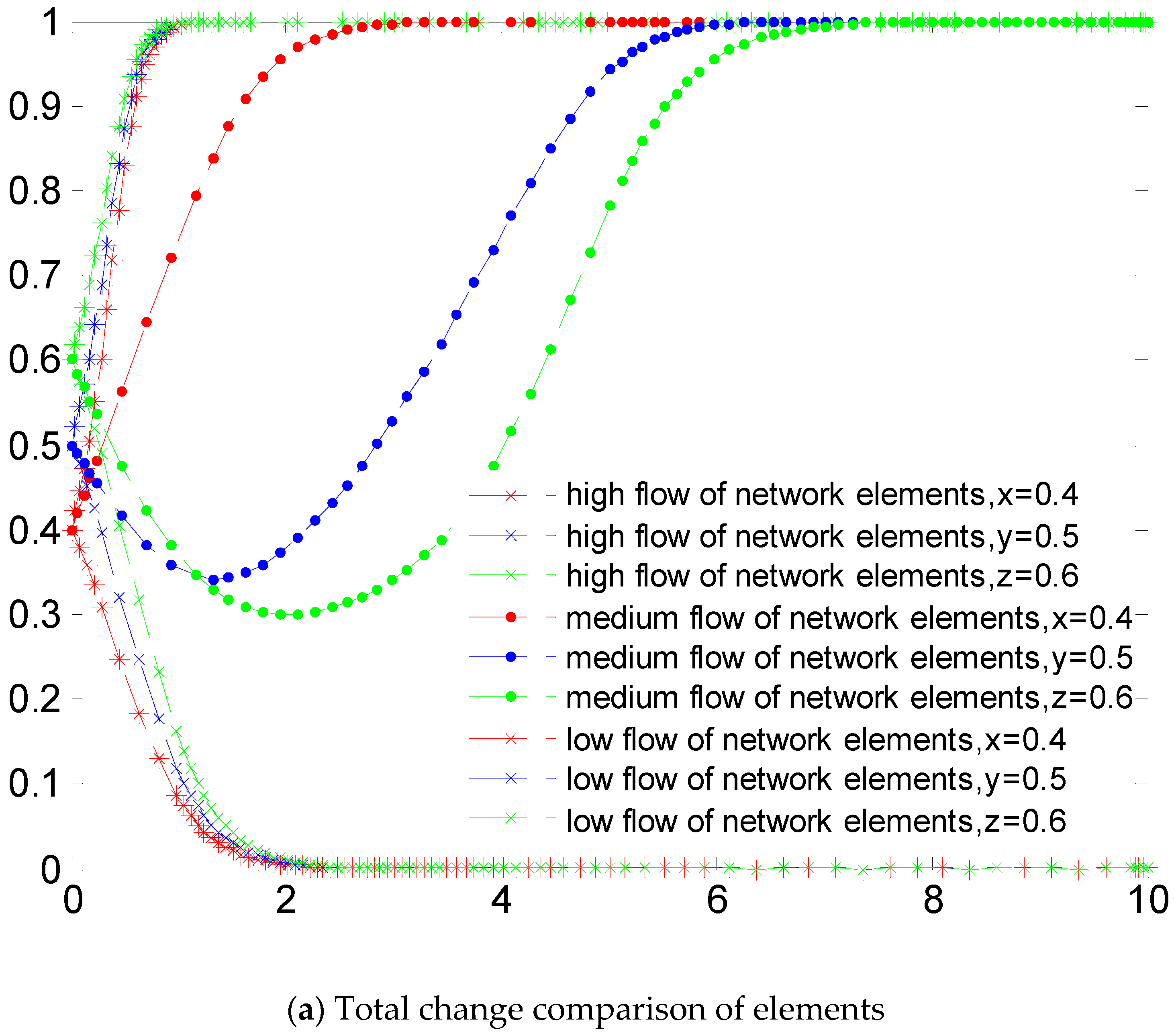
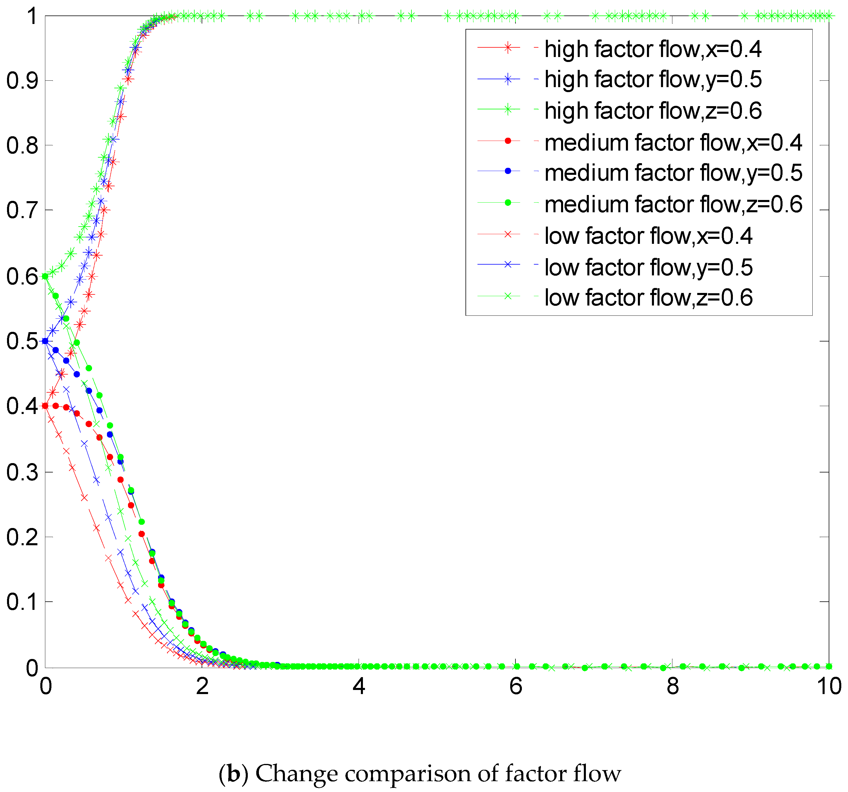
Conclusion 2.

In air pollution control, the total amount of network production factors (capital, technology, and information) and total network factors of production that can be moved production factors of local governments have a direct influence on the choice of behavioral strategies. Under the condition of the constant fixed cost of local governments, higher total network production factors and the flowable network production factors make the governments inclined to choose active cooperative behavioral strategies. Conversely, governments are inclined to choose a passive behavioral strategy. It can also be simply understood that with higher levels of air pollution control or factor spillover from local governments, the benefits of the active cooperative behavioral strategy are greater than the passive behavioral strategy. As a result, the willingness of local governments to cooperate has grown stronger.

Combined with Theorem 2–6, the choice of cooperation strategy is compared by varying the total amount of network production factors or the total amount of total network factors of production that can be moved according to the parameter assumptions, with a constant fixed cost of active cooperation and passive behavioral strategies of the three local governments. For the sake of clarity, it is assumed that all three local governments are homogeneous at high and low levels. If the fixed cost ${\eta }_i-{\mu }_i=-3,i=1,2,3$, the total number of network elements has three degrees: high ${\alpha }_i=4,{\beta }_i=2,{\gamma }_i=3$, ${\tau }_i={\psi }_i=1,i=1,2,3$; medium ${\alpha }_1=4,{\beta }_1=2,{\gamma }_1=2,{\alpha }_2=1.5,{\beta }_2=0.5,{\gamma }_2=1,{\alpha }_3=1.5,{\beta }_3=0.5$, ${\gamma }_3=1,{\tau }_i={\psi }_i=1$, $i=1,2,3$; low ${\alpha }_i=1,{\beta }_i=1,{\gamma }_i=0.5$, ${\tau }_i={\psi }_i=1,i=1,2,3$. Similarly, when setting the fixed cost to a fixed value, the flow of network elements has three degrees: high ${\alpha }_i=2,{\beta }_i=1,{\gamma }_i=1$, ${\tau }_i={\psi }_i=3,i=1,2,3$; medium ${\alpha }_i=2,{\beta }_i=1,{\gamma }_i=1,i=1,2,3$, ${\tau }_1={\psi }_1=2,{\tau }_2={\psi }_2=1.5,{\tau }_3={\psi }_3=0.5$; low ${\alpha }_i=2,{\beta }_i=1,{\gamma }_i=1$, ${\tau }_i={\psi }_i=0.3,$$i=1,2,3$. 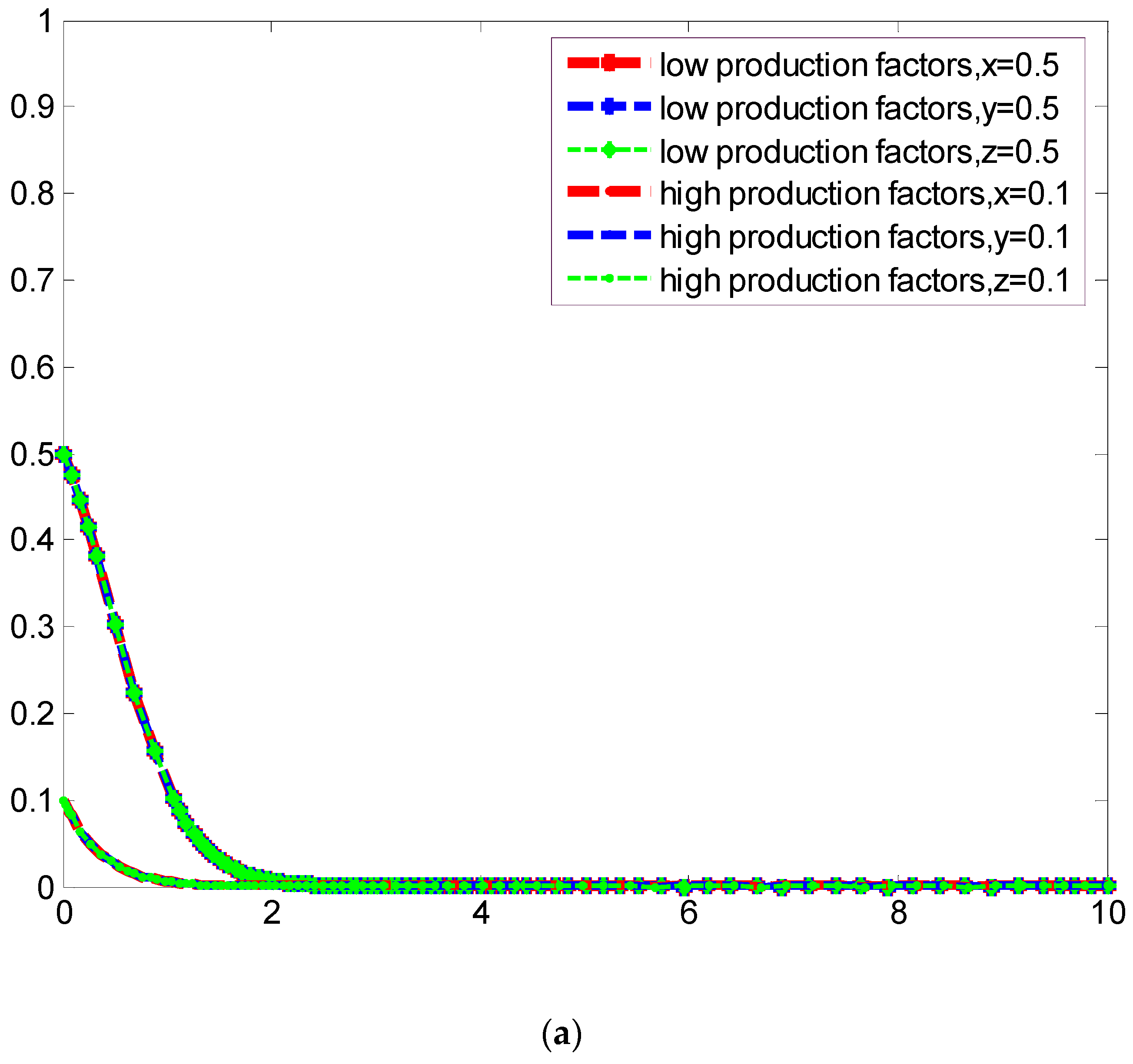The paths of its evolution are shown in Figure 3a,b.

Figure 3a,b show that, when the total amount of network production factors (pollution control level) and the total amount of network production factors that can be moved factors (openness of the government) are relatively high, the income of local governments choosing active cooperation is higher than that of local governments choosing passive treatment. This is true even when the fixed cost of local government remains constant. The primary cause is that local pollution control places more emphasis on the positive effects that environmental regulation has on the economy and external society. The three various behavioral strategies of the local governments are ultimately determined by the starting wishes and pertinent parameters of the local governments when the total network production factors of the local governments and the flowable network production factors are at a medium level. Local governments are, nevertheless, inclined to embrace active cooperative behavioral techniques when the advantages of doing so outweigh those of passive therapy. Local governments must incur certain costs for air pollution management, which results in short-term economic losses, when the total number of network production elements and the total network components of production that can be relocated by local governments are at a low level. As a result, local governments are likely to select a passive treatment strategy.

Intergovernmental collaboration is also primarily influenced by imbalances in local government pollution control and local government external transparency. In order to make up for cost losses, encourage the government to open up to the outside world, and enhance the active cooperative behavior of local governments, the state must provide certain policy incentives when local government governance is at a low level.

Conclusion 3.

According to Theorem 3–6, the initial cooperation probability of the three parties and the total production factors have an impact on the system’s ESS when local governments’ total production factors are equivalent (the pollution control level is consistent) in the intergovernmental cooperation on joint prevention and control of air pollution.

When the local government’s overall production factors are minimal or the tripartite cooperation’s original intentions are weak, the system’s ESS displays a tendency of (0,0,0). The ESS of the system is correlated with the probability of initial tripartite cooperation when the total production factors of local governments in the area are equal and at the medium level, and various evolution possibilities are possible. Therefore, the amount of regional economic development and the desire of local governments to collaborate have an impact on the effectiveness of intergovernmental cooperation in avoiding and regulating air pollution.

Theorem 3–6 states that when genuine production factors are low or when the initial willingness of the three parties is weak, parameters in joint prevention and control of air pollution take the evolutionary trend of the system ESS. The starting chance of cooperation between the three parties is set at 0.5 when production factors in the region are equal and minor. When the fixed cost is ${\eta }_i-{\mu }_i=-3,i=1,2,3$, the total network element is ${\alpha }_i=1,{\beta }_i=1,{\gamma }_i=0.5$, ${\tau }_i={\psi }_i=1,i=1,2,3$. When the production factors of the regional government are equivalent and large, set the fixed cost ${\eta }_i-{\mu }_i=-3,i=1,2,3$, the total network element is ${\alpha }_i=4,{\beta }_i=2,{\gamma }_i=3$, ${\tau }_i={\psi }_i=1,i=1,2,3$. 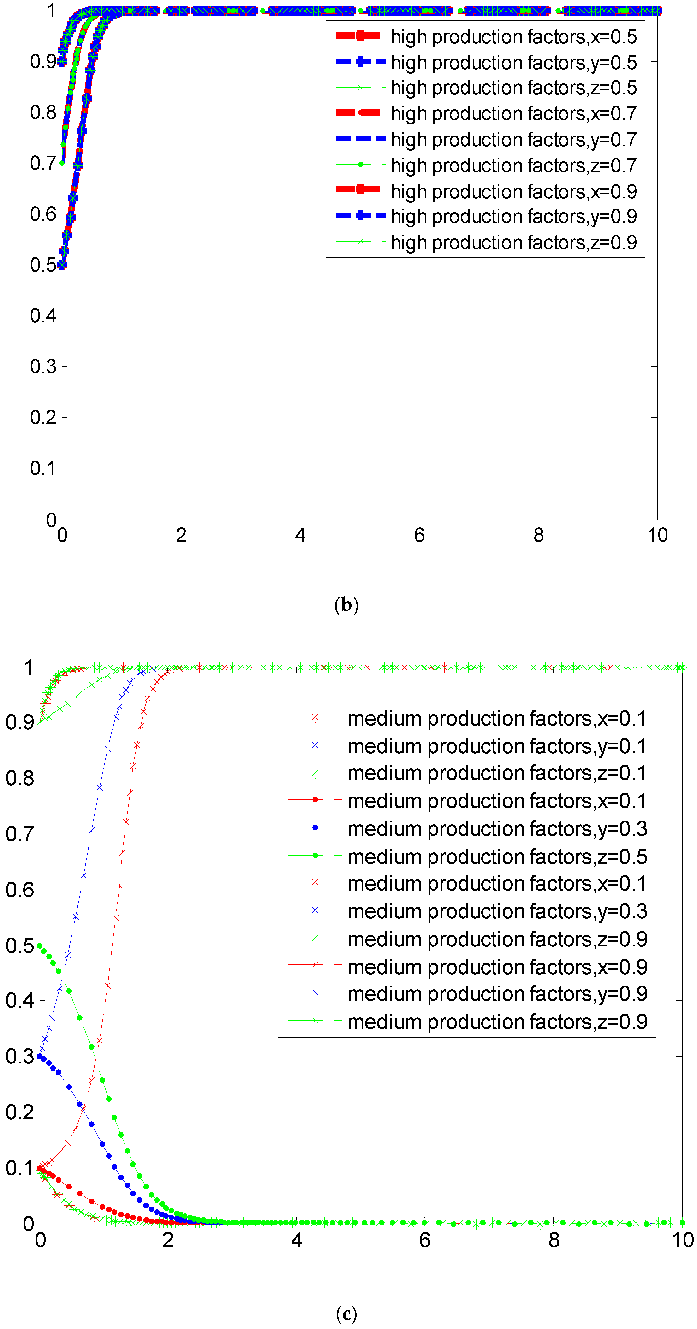However, when the initial cooperation probability of all three parties is 0.1, the evolutionary trend of the system ESS is shown in Figure 4a.

Afterward, the evolutionary trend of system ESS is simulated through parametric assumptions when the total production factors are large and the initial willingness of the three parties is strong. When the production factors of local governments are equal and large, the initial cooperation probability of the fixed three parties is 0.5, 0.7, and 0.9. When the fixed cost is ${\eta }_i-{\mu }_i=-3,i=1,2,3$, the total number of network elements is ${\alpha }_i=4,{\beta }_i=2,{\gamma }_i=3$, ${\tau }_i={\psi }_i=1,i=1,2,3$. The evolutionary trend of system ESS is shown in Figure 4b.

Finally, the parameters assume that the evolutionary trends of the simulated production factors of the system ESS are equivalent at the medium level. When the total production factors in the region are equivalent and at the medium level, the initial cooperation probability of the fixed three parties is (0.1, 0.1, 0.1), (0.1, 0.3, 0.5), (0.1, 0.3, 0.9), and (0.9, 0.9, 0.9). When a fixed cost is ${\eta }_i-{\mu }_i=-3,i=1,2,3$, the total network element is ${\alpha }_i=3,{\beta }_i=2,{\gamma }_i=2$, ${\tau }_i={\psi }_i=1,i=1,2,3$. The evolution trend of the system ESS is shown in Figure 4c:

Figure 4a–c show that the starting goal of cooperative governance in joint collaboration has a significant influence on the outcomes. If the local government initially expresses a willingness to cooperate but ultimately decides against it because there is no external incentive policy, the cost of collaborative governance is significant when the degree of local government control is at a low stage of development. Even though the governance is at the general level, local governments will eventually decide not to participate if there are no other pertinent external factors when their initial readiness to cooperate is relatively modest. Local governments have a certain initial inclination to collaborate when the level of local government governance is at a high stage of growth. Local governments will typically select collaboration because the advantages outweigh the opportunity costs. When local government control is at a general level, the local government’s ultimate behavior will depend on its initial willingness to cooperate. As a result, when the three parties’ initial willingness to collaborate is low, they will ultimately decide not to cooperate; when it is strong, they will ultimately decide to cooperate. However, there may be several evolutionary outcomes when the three parties’ initial willingness is incongruent.

As a result, in intergovernmental collaboration on joint air pollution prevention, the initial willingness to cooperate also plays a major role in influencing the final behavioral choice. Local governments must increase their initial willingness to cooperate once they have achieved a particular degree of governance through incentives or pressure from the federal government to encourage the prospect of intergovernmental collaboration.

Even though this study came to some important results, there are still issues and areas that need to be explored. In the future, we can approach things from the following angles: (1) This article solely takes the local government into account as the primary entity of collaborative governance due to space constraints. The evolutionary game concept is extended to incorporate higher-tier municipal governments, the general public, etc. (2) This paper ignores the effects of the cost of environmental protection itself and benefit income on the development of intergovernmental cooperation, focusing instead on the “benefit–cost” interest relationship between the network of intergovernmental cooperation for the joint prevention and control of air pollution. (3) Global cooperation in the prevention and control of air pollution. The environment of local intergovernmental collaboration and the environment of global coordination and cooperation for continued expansion is obviously different, even though this study has some implications for the control of air pollution.

5. Conclusions

By creating an evolutionary game model of joint prevention and control of air pollution, this research investigates the evolutionary process of local government behavioral strategy choice from the perspective of social public governance. In addition, the whole network of production elements that can be transferred, fixed capital, and the total production factors are all added to the payment matrix. Through three-dimensional dynamic system analysis and simulation, their effect on the collaboration of air pollution prevention and control is investigated. According to the pertinent numerical simulations and assessments: ① local government should consider fixed revenue and fixed cost when deciding on cooperative behavioral solutions for reducing air pollution. Collaboration must be the only tactical option for the tripartite local governments when the fixed income of the choice of cooperative behavioral strategy is higher than that of passive treatment of behavioral strategies. ② The relationship between local governments is dynamic and evolves through time as a result of elements such as total network production factors and total network production factors that are mobile. ③ In terms of preventing and controlling air pollution, the effectiveness of intergovernmental collaboration is influenced by the degree of regional governance and is strongly correlated with the local government’s willingness to cooperate. ④ The level of regional administration has a significant impact on intergovernmental collaboration in the joint prevention and control of air pollution, but so does the local government’s cooperation readiness.

The above research conclusions have a certain reference value for intergovernmental cooperation in joint prevention and control of air pollution. When formulating follow-up-related policies, on the basis of promoting the effect of joint prevention and control of air pollution and improving the level of network element spillover, local governments should be encouraged to have strong initial cooperation. willingness, and actively reduce the fixed costs of its governance. In reality, the collaborative management connection between local governments should be specified, and a collaborative management network should be built, in the collaborative air pollution management. In this process, we must first make clear which local government subjects are required to participate and provide them with a clear position based on their own willingness to cooperate, spillover level, and production factors. After that, we must allot benefits to them in accordance with the pay-and-gain principle before establishing a solid relationship, clear communication, and effective network for the collaborative management of air pollution.

Although this study came to some significant results, there are still flaws and uncharted territory, and the future can be viewed from the following angles. (1) The higher level of local government and the public can be incorporated into the evolutionary game model for future investigation. This paper solely addresses the local government as the primary body of collaborative governance due to space constraints. (2) This paper focuses on the “benefit–cost” relationship between the network of intergovernmental cooperation for the prevention and control of air pollution, but it ignores the price of environmental protection and the influence of revenue on the development of intergovernmental cooperation, both of which can be further investigated in the future. (3) Although this study has some implications for air pollution control, it can be elaborated upon by pointing out that there are important distinctions between the local intergovernmental cooperation environment and the international coordinating cooperation environment.