Abstract
Inventory management seeks to improve manufacturing by contracting inventory costs in a similar fashion to raise efficiency and profit. One approach is to develop inventory management models according to actual production systems. Furthermore, governmental policies in many countries impose many regulations on firms to fulfill the growing demand for a reduction in carbon emissions. Warm-up is a familiar concept in industrial applications. It allows the manufacturing system to work at a higher level of productivity and efficiency, as well as decreasing the number of defective items and maintenance costs. Along with fewer poor-quality items, the system has less waste as scrap items entering the environment and also requires less energy and workload to focus on reworking. The economic production quantity (EPQ) problems with a warm-up as an input parameter have been studied in a few works recently. This paper proposes a production-inventory model which considers the warm-up period as a decision variable and investigates its impact on the total cost. Furthermore, the defective rate is a decreasing linear function related to the warm-up period’s length. The production-inventory model takes into account the carbon emission tax policy. The main aim of this research is to jointly optimize both the length of the warm-up period and the production cycle in order to minimize the total cost of the production-inventory system and, therefore, reduce emitted carbon emissions. The comparison of tax prices and the effect of the proper warm-up period on the amount of carbon emissions are discussed in the sensitivity analysis.
1. Introduction
Two concerns are increasing among policymakers about the growing population: the need for more products and the global warming caused by carbon emissions. In addition, companies compete to do their best to provide better outcomes concerning powerful features such as final price, delivery time, and management policies. Achieving the balance between them can be obtained via inventory management. It is known as a critical factor in joint production and financial management, decreasing costs and in turn increasing profit.
On the one hand, climate change and global warming have disruptive impacts on human life. Many approaches are applied to control the total carbon emissions in any activity, including manufacturing systems. Decision makers suggest that governments can help this growing concern by levying taxes. As a result, some managers consider this issue as a decisive factor in their cost (Mishra et al. [1]). On the other hand, researchers developed traditional inventory management approaches for conditions such as defective items. One of these is the economic production quantity (EPQ) inventory model, which deals with the cost of production and the cost of holding items. This is the oldest and most well-known traditional model in production-inventory problems (Vidal [2]).
The concept of EPQ was structured upon some assumptions, which stand for mathematical equations, solutions, and optimizations to apply in practical situations. In most EPQ problems, the machine or manufacturing system starts from a constant rate of manufacturing in time. However, there are some machines or industries that work in different conditions. For example, a CNC (computerized numerical control) machine needs a short period to reach the predefined velocity.
Like the human body, which requires a period to prepare for a high-pressure activity, some industrial machines need warm-up time for the production cycle. For instance, Harmatys et al. [3] investigated the effect of the warm-up time on optical coordinate measuring machine measurement accuracy, and they showed that using coordinate measuring machines (CMM) is a common approach in industrial practices to check the quality of work pieces. This device can be affected by thermal expansion or other factors and has many derivations of the exact measuring. They utilized some experiments to examine the influence of the delay time from turning on the machine until it reaches a stabilized temperature. This period is used for warming up the machine in order to stabilize its temperature. They found that if there exists a lower amount of uncertainty then the machine must be warmed up.
Frigerio and Matta [4] surveyed the energy consumption of a manufacturing system according to different control policies. In CNC machining, they consider two types of warm-ups with constant and exponential functions. They assumed four states for the machine: out-of-state, warm-up, on-service, and working. The order of the states is represented in Figure 1. By considering a warm-up duration dependent on time and experimental work on the real CNC machine, one of the results is that with a shorter warm-up duration, the machine will be switched off sooner.
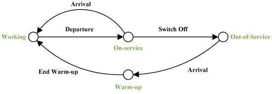
Figure 1.
The order of four states (Frigerio and Matta [4]).
Integrating warm-up into production-inventory systems gives production lines some benefits. In addition, warm-up is inevitable in many cases and is a great approach to obtain many advantages. The goal of warm-up can be divided into the three following cases:
Firstly, on the one hand, the warm-up can reduce the number of poor-quality items manufactured during the production run. This concept is well-known among ordinary people for machinery devices such as cars, which are supposed to decrease costs related to maintenance. On the other hand, working in a lower condition than the service rate enables a machine or any mechanical device to tolerate more pressure under a high serviceability period. In some cases, a period is considered to repair items and check the serviceability between the end of the warm-up and the start of the leading manufacturing process. In this period, production is interrupted for a short time with no products, so the rate of manufacturing is lower than the primary production. Afterward, the manufacturing line starts to work at the rate of the primary production (Nobil et al. [5]).
Secondly, expecting more efficiency is another consequence of providing a warm-up. Less maintenance service means fewer particles can be damaged, so the life span of machines will be extended. In addition, the serviceability of any mechanical devices and machines is related directly to oil which is used to reduce friction between two or more particles. Warm-up is a way to enable the oil to reach a specific temperature (Burke et al. [6]).
Thirdly, some industries, such as CNC machining, need to reach a fixed condition to start working. Machine tool spindles need to be heated to reach their service condition, and this time is necessary and studied (Li et al. [7]). Warm-up is an essential part of the process. As a result, with a sufficient amount of warm-up, the life span of manufacturing machines is extended and providing more efficiency and serviceability (Wang et al. [8]).
In addition, the warm-up period should not be considered a constant input parameter and the effective duration to maximize its benefits for the production system should be obtained (Frigerio and Matta [4]). Hence, this study presents an EPQ inventory model for a production system that runs with a warm-up period. The duration of the warm-up period in this system affects the fraction of poor-quality items produced and, subsequently, affects the production rate. The biggest contribution factor in this study is that the warm-up period is not a constant input parameter and was developed as a decision variable. The consideration of carbon emissions is included as a tax in the total cost of the manufacturing system. Furthermore, a mathematical function is used that has a relationship between the duration of the warm-up and the number of poor-quality items. The rest of the current paper is set as follows. Section 2 provides a literature review of the EPQ problems by focusing on the warm-up period. Section 3 presents the notation and formulation of the proposed EPQ inventory model. Section 4 develops the solution procedure to optimize the EPQ inventory problem. Section 5 solves a numerical example and does a sensitivity analysis. Finally, Section 6 includes the conclusion of this study and the future works that can be done.
2. Literature Review
The application of a warm-up in inventory management practice is very pioneering, and there are few research papers in this area. By studying the warm-up, it is necessary to define the manner of how to implement it in an EPQ inventory model and then give insights to other researchers to pay attention to this unexplored field in the production-inventory models.
The beginning of inventory management started with the fundamental inventory model proposed by Ford Whitman Harris in 1913. He presented the first economic order quantity (EOQ) inventory model with a simple assumption that demand has a constant rate. This idea was ignited in his mind due to reaching a balance between the costs of carrying inventory and ordering. Although this story was forgotten in the scientific area, the hard-working of some researchers found his work and identified his contribution to the inventory field. His inventory model is also popular with the name “square root formula”. Five years later, in 1918, Taft made a significant development in the field of inventory management and introduced a new variant of the EOQ classical concept under another assumption. This is the emersion of economic production quantity (EPQ) in technical literature. This is because of considering a finite rate of production for EOQ problems (Andriolo et al. [9]).
The new era of inventory management was created by the contributions of several researchers around the world; those inventory models have simple assumptions which are studied to understand the whole concept of this field. The focus was just on decreasing the costs related to inventory and holding of items. After a century, researchers found some weaknesses in Harris’s and Taft’s assumptions, which are not related to real-life situations. By investigating each assumption in these inventory models, a new field of study with a tremendous amount of work was created. Most recent studies of EPQ problems are categorized into the six following groups:
- (I)
- A company or firm can use a multi-item production system in its process. Multiple products help the inventory system with higher usage of machine tools utilization and overcome uncertainty related to single products such as the generation of poor-quality items. Chiu et al. [10] proposed a producer-retailer incorporated multi-product lot size problem with delayed differentiation. Nafisah et al. [11] addressed a multi-product inventory EPQ problem with time-dependent pricing and rework costs. Soleymanfar et al. [12] have another paper in this field that has considered the influence of return policy for sustainable multi-product EOQ and EPQ inventory models.
- (II)
- Several inventory systems deal with products that can deteriorate over time such as food and dairy products; some research focuses on the trade-offs of these items with the total cost. Supakar and Mahato [13] built an EPQ model with time proportion deterioration and ramp-type consumption under various payment schemes. Lu et al. [14] investigated the influence of the carbon emission policy on the optimal production-inventory decisions for deteriorating items. Barman et al. [15] published a paper on deteriorating items and evaluated the effects of preservation and green technology investments on a sustainable lot sizing model during the COVID-19 pandemic.
- (III)
- Even the highest quality machines produce a number of imperfect items. This amount is a manufacturing concern that can be reworked or scrapped. The rate of production of these items or the total number of them can be decisive in EPQ inventory models. Guatam et al. [16] determined the optimum production-inventory strategies for a flawed production system with price-reliant and advertisement demand under the rework option for defective items. Giri and Dash [17] derived an optimal batch shipment policy for a flawed production system with price, advertisement, and green-sensitive demand. Tayyab et al. [18] published an economic assessment of a serial manufacturing system with random imperfection and backorder.
- (IV)
- Demand is an essential part of each inventory system. Shortage can occur when demand increases along with the population growing day by day or when the amount of produced items cannot fulfill the defined demand. Poswal et al. [19] examined and evaluated a fuzzy EOQ inventory model for price-sensitive and stock-dependent demand under shortages. The other work is from Hou et al. [20], who considered an EPQ problem with maintenance and shortages of deteriorating items. Alarjani et al. [21] developed a sustainable optimal recycle quantity model for a flawed production system with shortages.
- (V)
- Companies utilize different policies to promote their products; one effective approach is an alternative payment method for retailers. A delay payment method is offered by the supplier to retailers as an incentive for selling more items. Trade credit policy is a common practice among most inventory systems. Wang et al. [22] proposed a two-level trade-credit mode and found the optimal trade credit and optimal order quantity through the Stackelberg game. Poswal et al. [23] developed a manufacturing model with trade credit policies. They considered some parameters such as carbon emissions and remanufacturing items to practice sustainable inventory management. Mandal et al. [24] developed an unreliable EPQ model with a two-level trade credit policy. In their model, demand is dependent on the selling price and their objective is to find the optimal profit.
- (VI)
- Another significant consequence of the development in EPQ problems is considering the environmental impact of manufacturing systems, particularly carbon emissions. Carbon emissions are produced and released into nature through any firm part (He et al. [25]). Furthermore, the amount of emission is different compared to other parts. According to Hua et al. [26], all firms should consider carbon emissions in their management. It is important to mention that the focus in this field has been increasing among researchers in recent years. Two regulations regarding carbon emissions are studied more in the literature of EPQ inventory models, cap-and-trade, and carbon tax (He et al. [25]). Dong et al. [27] conducted a case study on China’s carbon emissions. They concluded that adopting a carbon tax policy is an effective policy to mitigate the concern of growing carbon emissions in the industry sector. Moreover, this policy has less impact on economic outcomes and welfare losses. A carbon tax policy was used by 21 countries or regions in the world, more than other policies (Zhou et al. [28]). This approach is simple to apply to any sector without advanced technology and is also easy to track for governments when the amount and the growth of carbon tax over time is more important (Carattini et al. [29]). This rate should be set more carefully so as not to have negative consequences on downstream manufacturers as well as on market competition (Zhang et al. [30]). Sinha and Modak [31] proposed an EPQ inventory model considering carbon emissions. They gained benefits from the plantation and provided trees for nature, undermining the negative impact of their carbon footprint. They concluded that as well as providing plantations, firms could produce more items. A survey on the sustainable EPQ inventory model with a partial backorder and full backorder was conducted by Taleizadeh et al. [32]. Mishra et al. [1] presented an inventory model to obtain the highest profit by investing in greener technologies and preserving them. This study applies Mishra et al.’s [1] approach to calculating carbon emission cost. Daryanto and Wee [33] formulated two EPQ inventory models to reduce carbon emissions. Basically, they considered carbon cost as part of their their total cost and then developed an inventory model with a shortage. Mukhopadhyay and Goswami [34] presented an EPQ inventory model with three different types of defective items and also two types of pollution costs. Table 1 shows some recent studies that include EPQ problems with the consideration of carbon emissions. It is worth mentioning that these research works do not include a warm-up period, except for this study.
 Table 1. Comparison among the inventory models in the literature of EPQ problems with carbon emissions.
There are only four related research works regarding EPQ problems that consider warm-up in the literature, and the primary approach and decisive variables with their conclusions are described in the following.
The first scientific study that considers the effects of the warm-up period on EPQ problems is presented by Nobil et al. [5]. They proposed an EPQ inventory model with a warm-up period for a cleaner production environment. Their objective was to examine the influence of the warm-up period on a defective inventory system. In this system, defective items gain perfect quality, and this can be helpful for the environment. This approach resulted in two problems, a convex programming problem and a concave programming problem, proving that there is an optimal solution. Finally, they proposed an exact solution algorithm for both.
Imperfect items in the production process can be reworked or disposed of as waste products. Bazan et al. [35] suggest companies reduce the amount of remanufactured products from environmental aspects. Furthermore, El Saadany et al. [36] considered factors that result in a negative impact on the environment including energy consumption and waste disposal. Defective items with both scenarios, if going for rework or disposal, have negative consequences. By using an adequate warm-up period, the manufacturing system runs with fewer defective items. In addition, the effect of higher efficiency for machine tools and longer lifespan results in less maintenance cost and workload. Obviously, less energy consumption would be used on maintenance.
Another work is also by Nobil et al. [37], which is about an EPQ problem for a single-machine inventory system. They considered the warm-up period for an economic lot scheduling problem (ELSP) and divided the production system into three subsystems: two single-item EPQs and one ELSP; this division is according to the relationship with production and consumption. Their objective was to reach the optimum cycle length to reduce the system’s total cost. Finally, they suggested an exact solution.
The third related paper in this field is proposed by Ganesan and Uthayakumar [38], which is related to inventory models for an imperfect manufacturing system considering the warm-up period and partial backordering during the hybrid maintenance period. Their paper includes two types of EPQ inventory models considering four cases: the warm-up process, hybrid maintenance schedule, amount of shortage during this, and rework of defective items. They used two different rates of production for defective items. They concluded that properly selecting a warm-up period and a hybrid maintenance scheme reduces the shortages during the maintenance period and the number of defective items. In addition, they suggested that the time of reworking defective items is a decisive variable in future works.
The fourth related investigation in this field is by the same authors, Ganesan and Uthayakumar [39]. In this paper, they chose a production inventory model and considered the warm-up process, the shortage during the hybrid maintenance period, and the rework for defective items. The number of defective items produced during the warm-up and regular process comes from a bivariate random variable. They investigated the influence of the learning capabilities of workers in the production line as a decisive parameter. Because of the high dimension of nonlinearity in these models, they used a genetic algorithm to solve the problems. The conclusion of this work pointed out that learning about the production system increases the production rate and decreases the amount of time needed for producing items.
All the related papers available on the concept of EPQ and considering warm-up are mentioned, and the critical aspects of their views are described. Table 2 presents the brief details of the papers with their comparisons.
Table 2.
Comparison of the EPQ problems with a warm-up.
As can be seen from Table 2, the warm-up period is considered a fixed parameter in most studies. Even though Ganesan and Uthayakumar [38] considered that the warm-up period is a variable, it only had an impact on the total cost, and it was not a function, i.e., this variable was only considered as the period of heating the machine. It was not important how long it took. In this study, the warm-up period is considered a decision variable. Its length affects the defective rate. The defective items are produced during the manufacturing process and considered scrap items. As a result, this paper studies an EPQ problem by considering the warm-up period as a decision variable, on which the defective rate is dependent. Finally, this study calculates the optimal length of the warm-up period and the cycle time and the optimal total cost.
3. Proposed Model
The notation of the production-inventory model of the current study is described as follows:
Parameters:
: Unit production cost (currency symbol/unit)
: Unit scrapped cost (currency symbol/unit)
: Setup cost per cycle (currency symbol/setup)
: Warm-up cost per unit of time (currency symbol/unit of time)
: Unit holding cost per unit of time (currency symbol/unit/unit of time)
: Demand rate per unit of time (currency symbol/unit of time)
: Production rate per unit of time (currency symbol/unit of time); : Maximum allowable fraction of poor-quality items
: Minimum allowable fraction of poor-quality items; ()
: Maximum allowable time for the warm-up period (unit of time)
: Carbon emission unit associated with each setup process (unit of weight/setup)
: Carbon emission for the warm-up period (unit of weight/unit of time)
: Carbon emission for production per item (unit of weight/unit)
: Carbon emission for disposal scrap item (unit of weight/unit)
: Carbon emission for inventory per item per unit time (unit of weight/unit/unit of time)
: Carbon tax (currency symbol/unit of weight)
Function:
: function of the fraction of poor-quality items with respect to warm-up period
Dependent decision variables:
: Maximum on-hand inventory level per cycle (units)
: Production quantity per cycle (units)
: Production period per cycle (unit of time)
: Consumption period per cycle (unit of time)
: Total emission cost of carbon (currency symbol/unit of time)
: Total cost without emission cost of carbon (currency symbol/unit of time)
: Integrated total cost (currency symbol/unit of time)
Decision variables:
: Cycle length (unit of time)
: Warm-up period (unit of time)
The graph of the on-hand inventory level of the production-inventory model is illustrated in Figure 2. Production rate () includes two kinds of items: good and poor-quality. The poor-quality items are produced with rate. The is a function of the fraction of the poor-quality items, which depends on the length of the warm-up period. This function is linear, and it relates to the fraction of the poor-quality items with the warm-up period, which is shown in Figure 3. As shown in Figure 2, once the production period () is stopped, the maximum inventory level is shown as ; after that, consumption period () starts at inventory level to zero. The maximum on-hand inventory level, production, and consumption periods are computed as follows:
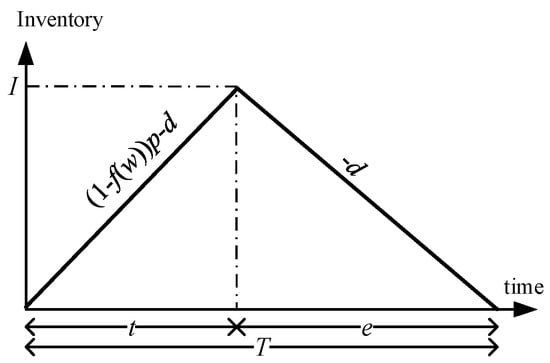
Figure 2.
Graph of the inventory level in the production-inventory model.
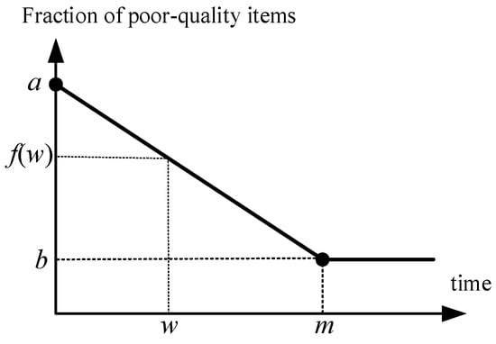
Figure 3.
Graph of the behavior of the function of the fraction of the poor-quality items.
Therefore, based on Equations (2) and (3), the cycle length is obtained as follows:
and
In this study, the warm-up period is considered a decision variable. In real-world practices, the amount of warm-up can be varied in a specified range. Neglecting a warm-up run before the main process results in a number of defective items due to the absence of the warm-up process’s benefits. As depicted in Figure 3, when the length of the warm-up period is zero, there is a maximum fraction of poor-quality items for the manufacturing system. The machine tools should run under a warm-up process for an adequate period. Surpassing the cap time does not turn into a benefit because of the intrinsic characteristics of any machine tool. Consequently, spending more than the cap time of the warm-up process results in wasting time and workload with a few imperfect items that cannot be got rid of during warm-up. In other words, the minimum fraction of poor-quality items occurs when the length of the warm-up period takes up to the maximum time allowed to warm up (). Therefore, the relation of the warm-up period with the number of imperfect items is considered with the linear function, and the function of the fraction of poor-quality items concerning the length of the warm-up period is as follows:
The total cost of the inventory system includes setup, warm-up, production, disposal, and holding costs. The calculation is shown as follows: the setup cost per cycle is monetary unit, and thus, the setup cost per unit of time becomes . The cost of the unit warm-up time is monetary unit, since the warm-up cost depends on the length of the warm-up period (), and thus, the warm-up cost per cycle is calculated as the warm-up cost multiplied by the length of the warm-up period (). Therefore, the warm-up cost per unit of time is obtained as . The production quantity in each cycle is , and is the production cost of each item. The production cost per cycle is equal to , and subsequently, the production cost per unit of time is . Now, using Equation (5), the production cost per unit of time is given by . Additionally, during the production period, there is an amount of produced items that it is not manufactured correctly and has poor quality. This amount is equal to ; thus, the disposal cost per cycle is , and the disposal cost per unit of time is Using Equation (5), the disposal cost per unit of time is computed as , where is the unit scrapped cost of each poor-quality item. The holding cost per unit of time is obtained by calculating the area of Figure 2 as . Substituting from Equation (1) into the holding cost, we have . Finally, the total cost of the inventory system without carbon emission consideration according to the setup, production, warm-up, disposal, and holding costs is as follows:
Now, the effects of carbon emission costs are added to the total cost in Equation (7) as follows: the total carbon emissions are calculated based on the carbon quantity emitted from the setup, warm-up, production, disposal, and holding processes. The carbon emission produced in each setup cost is . Thus, the unit of time’s carbon emission associated with the setup process is . Furthermore, the carbon emission of the unit warm-up time is , and thus, the carbon emission of the warm-up process is calculated as . The carbon emission emitted for manufacturing per item is , and thus, the total carbon emissions generated by manufacturing all the items is equal to . Additionally, the carbon emission produced during disposal of each poor-quality item is ; then, the total carbon emissions made for all the poor-quality items is equal to . The carbon emissions emitted from the holding process are obtained as . Therefore, the total emission cost of carbon for setup, warm-up, production, disposal, and holding processes is as follows:
Now, we can obtain the total integrated cost of the proposed model according to the total inventory cost in Equation (7) and the total emissions cost of carbon in Equation (8) as follows:
In this production system, the warm-up period happens at the end of the consumption period because after that the production period starts. Therefore, the warm-up period should be smaller than the consumption period, as follows:
Substituting from Equation (3), we have ; then, using Equation (5), this constraint is . Finally, by substituting from Equation (6), this constraint is as follows:
On the other hand, if the warm-up period is longer than the maximum allowable time, it is not practical. Therefore, the warm-up period occurs between its set limit, i.e., . Finally, based on the objective function and the constraints, we can provide the final model as follows:
where is
4. Solution Procedure
This section firstly proves the convexity of the objective function (12) using the Hessian matrix, and subsequently, according to the linear constraints, the proposed minimization model is proved, which is convex. Therefore, we calculate the partial differentiations of the model as follows:
Now, from (15), (17), and (18), the calculation of the Hessian matrix is as follows:
Theorem 1.
The hessian matrix of the objective function in (12) is positive.
Proof.
All parameters in (19) are positive. Based on the assumptions of the proposed model, , where is , then, , , , and . Therefore, all the terms in Equation (19) are positive, and subsequently, the Hessian matrix (19) is positive definite for all non-zero and .
Since the Hessian matrix of the objective function (19) is positive according to Theorem 1, the objective function (12) is convex. Subsequently, the proposed model is a convex programming problem because the model’s constraints are linear and, hereupon, convex. To obtain the optimal value of the cycle length and the warm-up period, we set Equations (14) and (16) to zero and solve the resulting concurrent equation system as follows:
□
We cannot find the optimal solutions in closed form from Equation (21), but the value of (20) can be put into (21), and hence, we can find the optimal value of the warm-up period using the Newton–Raphson method. After that, it is possible to determine the optimal value of the cycle length using (20). Additionally, we need to check the following two constraints of the problem and to make sure the solutions are feasible. Furthermore, the percentage of the defective range based on warm-up length and must be updated based on the relationship between the production rate and the demand rate to have a feasible solution. Therefore, we suggest the following solution procedure:
- Step 1.
- Check feasibility:
- Step 1.1.
- If , the problem has a feasible solution and goes to Step 1.2; otherwise, the problem has no feasible solution.
- Step 1.2.
- If , so the problem has a feasible solution and goes to Step 2; otherwise, go to Step 1.3.
- Step 1.3.
- When , we must ensure that the amount of heating length is calculated in such a way that no shortage occurs. Thus, we update the lower limit of the warm-up period as , and hence, , and go to Step 2.
- Step 2.
- Substitute (20) into (21), and hence, find the value of using the Newton–Raphson method.
- Step 3.
- If , so ; otherwise, , and go to Step 4.
- Step 4.
- Based on the value of , determine the values of and using (13) and (20), respectively.
- Step 5.
- If , so ; otherwise, , and go to Step 6.
- Step 6.
- Based on the values of and , obtain the optimal value of from (9).
5. Numerical Example and Sensitivity Analysis
To demonstrate the result of the work of this study, we apply the proposed exact solution approach to solve the following numerical example: Let /setup, /unit, /scrapped unit, units/shift, units/shift, /unit/shift, /shift, shift, /kg, kg/setup, kg/shift, kg/unit, kg/unit, kg/unit/shift, , and . We consider that the shift is 8 h.
According to the above data, the warm-up function of this system would be 0.2. Firstly, we ensure that the problem has a feasible solution as follows: . Then, using Equations (20) and (21), let us apply the Newton–Raphson method, and the length of the warm-up period is obtained as 0.149 shifts (please see this point in Figure 4). This length is less than the maximum allowable time for a warm-up period, , so that the optimal warm-up period would be equal to this length, i.e., 0.149 shifts. Then, based on the optimal value of , the value of and are computed using Equations (20) and (13), respectively. These values are 2.188 shifts and 0.212 shifts. Since , the optimal cycle length would be 2.188 shifts. Therefore, 650.814 items and the optimal value of the total carbon produced per shift () is equal to 2341.215 kg.
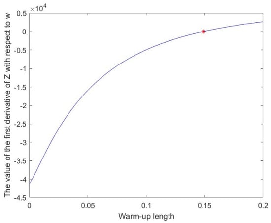
Figure 4.
Plot of the value of the first derivative of the objective function with respect to the warm-up length.
Finally, according to the optimal values obtained using Equation (12), the optimal total cost of the system is 7460.679.
Without consideration of the carbon emission amount, in this example the optimal warm-up period, optimal cycle length, and optimal total cost, respectively, are as below:
Without carbon emissions (if ), 0.196 2.919 shifts,
738.987 items, and 6182.319.
According to the results, using the carbon tax approach costs about 7460.679 − 6182.319 = 1278.36 $ for firms. This portion is meaningful when more than fifteen percent of the business’s overall cost comes from environmental impact. The governments can afford to invest in facilities or plantations to offset the negative impact of carbon emissions. In addition, managers can decide on some solutions to decrease their portion in producing pollution.
By putting 0.196 shifts and 2.919 shifts in the problem with carbon emissions, we have 739.979, 2857.404 kg, and 7611.174. Obviously, the optimal total cost obtained without carbon emissions is more than the optimal total cost derived from the consideration of carbon emissions.
Considering this problem without the warm-up period () results in a classic EPQ problem with rework, 0.898 shifts, 598.666 items, and 9412.221. Therefore, this EPQ problem with warm-up can reduce 9412.221 − 7460.679 = 1951.542. This portion is meaningful when more than twenty-five percent of the overall cost of businesses comes from the warm-up impact.
Figure 5 illustrates the plot of this numerical example’s objective function according to the limits of the variables.
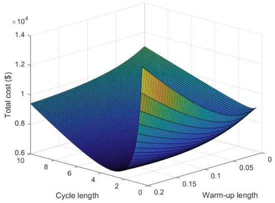
Figure 5.
Plot of the objective function of the numerical example.
5.1. Sensitivity Analysis
We consider all input parameters of the proposed model to analyze their effects on the optimal solutions. These parameters are expressed in three categories: cost, carbon emissions, and the other parameters. They are shown respectively in Table 3, Table 4 and Table 5.
Table 3.
Sensitivity analysis of the cost parameters.
Table 4.
Sensitivity analysis of the carbon emission parameters.
Table 5.
Sensitivity analysis of the other parameters.
As can be seen in Table 3, the minimum limit of the cycle length is changed moderately with direct variation of the setup cost, production cost, and scrapped cost. Furthermore, it has a moderately reverse relationship with changes in holding cost and warm-up cost, and carbon tax. The trend for the optimized warm-up period is highly dependent on changes in setup cost, production cost, and scrapped cost and has a high reverse relation with holding cost and warm-up cost and carbon tax. Optimized cycle length is slightly affected by changes in setup cost, production cost, warm-up cost, and scrapped cost. This is true with the reverse relation for holding cost and carbon tax. The production quantity has a direct relation to changes to setup cost and warm-up cost. In contrast, it is reversely affected by changes to production cost, scrapped cost, holding cost, and carbon tax. The amount of carbon emission changes with variation of setup cost, production cost, scrapped cost, holding cost, warm-up cost, and carbon tax. Optimized total cost varies slightly via changes in the following parameters: setup cost, production cost, and scrapped cost. It has a reverse response to changes in holding cost, warm-up cost, and carbon tax.
From Table 4, it is inferred that the minimum limit of the cycle length and optimized warm-up period moderately change according to the carbon emission associated with each setup process and the carbon emission for production per item and disposal per scrap item. In addition, it has a moderate reverse relation with the carbon emission for the warm-up period and inventory per item.
The optimized cycle length slightly varies according to the carbon emission associated with each setup process, warm-up period, production per item, and disposal per scrap item. It varies reversely with the carbon emission for inventory per item. The production quantity directly changes with slight differences of carbon emission associated with each setup process and the carbon emission for the warm-up period, whereas it shows the reverse effect with changes to carbon emission associated with production per item, disposal per scrap item, and inventory per item. The amount of carbon emission changes slightly with all parameters, including carbon emission associated with each setup process, the warm-up period, production per item, disposal per scrap item, and inventory per item. The optimized total cost changes considerably with variation of all parameters, including carbon emission associated with each setup process, the warm-up period, production per item, disposal per scrap item, and inventory per item.
In Table 5, the rest of the parameters are described with their effects. The minimum limit of the cycle length was highly affected by the change in maximum allowable time for the warm-up period, the minimum allowable fraction of poor-quality items, the demand rate, and the maximum allowable fraction of poor-quality items. Nevertheless, the production rate has a slight reverse relation. The optimized warm-up period moderately varies when changes occur in following parameters: the maximum allowable time for the warm-up period, the minimum allowable fraction of poor-quality items, the maximum allowable fraction of poor-quality items, and the production and demand rate. The optimized cycle length was moderately effected by variation of the maximum allowable time for the warm-up period, the minimum allowable fraction of poor-quality items, and the maximum allowable fraction of poor-quality items. This trend shows a reverse effect via changing the production rate and demand rate. The production quantity changes directly when changes occur in the maximum allowable time for the warm-up period, the minimum allowable fraction of poor-quality items, the demand rate, and the maximum allowable fraction of poor-quality items. However, a reverse effect to changes in the production rate was shown. The amount of carbon emission varies moderately when changes happen to the maximum allowable time for the warm-up period, the minimum allowable fraction of poor-quality items, the production rate, the demand rate, and the maximum allowable fraction of poor-quality items. The optimized total cost shows slight changes from all input parameters, maximum allowable time for the warm-up period, the minimum allowable fraction of poor-quality items, the production rate, the demand rate, and the maximum allowable fraction of poor-quality items.
In the actual situation, since the warm-up period usually is much lower than the production time, the effects of change in the value of the warm-up period have slightly more effect on the model than the effects of change in the value of the production time or rate and this can be seen in the tables as well.
5.2. Managerial Insights
This study helps managers to accurately define the period of production and warm-up and decrease total cost. By setting the correct period for the warm-up process, it is possible to maximize the system’s benefits. For example, based on the numerical example presented in this study, consideration of the warm-up process in the manufacturing system can provide about a 26 percent reduction in total cost. In addition, the effect of the warm-up period on the total cost was calculated, and managers can track the changes to obtain the proper value for their systems. The optimal value for cycle time and order quantity allows them to decide upon the provided equations and have a greener manufacturing system. This study gives an insight for the companies that seek minimize their cost along with considering the environmental issues. Moreover, decision makers can decide upon the consideration of carbon tax for manufacturing systems. This research made a comparison of the difference of the utilization of the tax policy for the system. The carbon tax policy costs 20 percent in this study for the system. Also, machines and devices work more efficiently with a sufficient warm-up period. As a result, a large portion of scrapped items will be diminished. In addition, the warm-up period can extend the lifespan of machines and systems. This can reduce costs related to repairs and maintenance as well as eliminating the need to spend on providing more machines. As a result, this research proposed an EPQ model that allows managers to use the concept of warm-up as well as the carbon tax policy and expend the minimized cost for their system.
5.3. Sustainability Aspects
The concept of sustainability has found great attention in the last three decades. The term “triple bottom line” has become popular in focusing on a sustainable approach consisting of three aspects: economic, social, and environmental (Glock et al. [40]). The warm-up period brings some consequences for a manufacturing system. This research performed a thorough study of the effect of a proper warm-up period on the total cost with consideration of carbon emissions. Money gained from decreasing total costs can be used to invest in new facilities such as green technology. Machine tools work more efficiently, which can diminish maintenance costs as well as production costs. The production process faces fewer scrap items. In addition, machine tools in the production line have a longer life span. With respect to the social aspect, with fewer defective items, the possibility of the occurrence of shortages will be decreased. The demand can be satisfied in time. As a result, customer and retailer satisfaction is ensured. The manufacturing line meets less workload due to fewer defective items; in addition, machine tools interrupt fewer times if they work efficiently. From the aspect of the environment, disposing of defective products requires more material for substitution, if they are considered scrap items. In this scenario, the system needs more material and items disposed of are wasted on the environment. Otherwise, they undergo a rework process that entails more energy to run. The consideration of carbon emission is the key point in this paper for sustainability performance. Applying carbon tax to the total cost results in an approach that provides optimized cost by considering the warm-up concept and carbon tax policy in an EPQ problem. It ensures the reduction of carbon emissions in this manufacturing system.
5.4. Environmental Insights
Machines work better with a sufficient warm-up period, and scrapped items are produced less. Thus, a lower amount of scrapped items will go into the environment and damage it. In addition, machines or devices nowadays work on fossil fuel or work using electricity in the best situation. Higher efficiency for these machines can reduce the fuel they need to use and reduce the pollution entering the environment. From the other aspect, utilizing the carbon emission cost in the total cost of the inventory system is a way to encourage managers to reduce their carbon emissions. This study integrated the inventory system and carbon emission approach into an EPQ problem with a warm-up period to optimize total cost.
6. Conclusions
The importance of warm-up is inevitable in many industrial practices. It can provide some features to a system, such as extending the lifespan of particles, fewer maintenance costs, and fewer defective items produced in the manufacturing line. We considered that the warm-up period is not fixed and presented mathematical equations concerning that. According to that, the defective rate was presented as a decreasing linear function of the length of the warm-up period. Thus, we formulated the EPQ problem with the warm-up function in a capacitated nonlinear programming problem. To address the most significant concern of today’s society, we considered carbon emissions in our study. The goal of this problem was to determine the optimal length of the warm-up period and the production cycle such that the total cost, including the cost of the inventory-production system and carbon emission, is minimized. Finally, we solved this model using an exact model and provided a numerical example to illustrate the applicability of the proposed problem.
The application of the warm-up period as a decision variable is a novel concept in the field of inventory management. By setting a value for the warm-up period, the cost and cycle time can be obtained. Furthermore, the effect of the carbon tax policy is applied and studied in this EPQ problem. The warm-up period can be a problematic process in the production run and provides advantages to an inventory system by increasing the effectiveness of the machine tools; in contrast, higher efficiency results in a lower number of poor-quality items. Truly, producing fewer waste products reduces the amount of the workload and the energy spent on reworking, and fewer waste products enter the environment. This study has some constraints in that setting the proper amount of warm-up is limited to the operator. Moreover, we consider that imperfect products are disposed of. For future work, the system could have a rework process for defective items. In addition, there are products that can deteriorate over time; this type of item could be considered to develop this study. Furthermore, the effect of downtime of the machine tools has not impacted on the warm-up period.
Some extensions for this study could be as follows: (a) considering several warm-up periods in each production cycle, (b) assuming the shortage is allowed, (c) investigating the effect of the machine shutdown time on the warm-up period, and (d) considering a production system with several products.
Author Contributions
Conceptualization, E.N., L.E.C.-B., I.d.J.L.-H., N.R.S., G.T.-G., A.C.-M. and A.H.N.; Methodology, E.N., L.E.C.-B., I.d.J.L.-H., N.R.S., G.T.-G., A.C.-M. and A.H.N.; Software, E.N., L.E.C.-B. and A.H.N.; Validation, L.E.C.-B.; Formal analysis, E.N., L.E.C.-B., I.d.J.L.-H., N.R.S., G.T.-G., A.C.-M. and A.H.N.; Investigation, E.N., L.E.C.-B., I.d.J.L.-H., N.R.S., G.T.-G., A.C.-M. and A.H.N.; Data curation, E.N. and L.E.C.-B.; Writing—original draft, E.N. and A.H.N.; Writing—review & editing, L.E.C.-B.; Visualization, E.N. and L.E.C.-B.; Supervision, L.E.C.-B. All authors have read and agreed to the published version of the manuscript.
Funding
This research received no external funding and the APC was funded by Tecnológico de Monterrey.
Institutional Review Board Statement
Not applicable.
Informed Consent Statement
Not applicable.
Data Availability Statement
All data are contained in the paper.
Conflicts of Interest
The authors declare no conflict of interest.
References
- Mishra, U.; Wu, J.Z.; Sarkar, B. A sustainable production-inventory model for a controllable carbon emissions rate under shortages. J. Clean. Prod. 2020, 256, 120268. [Google Scholar] [CrossRef]
- Vidal, G.H. Deterministic and Stochastic İnventory Models in Production Systems: A Review of the Literature. Process Integr. Optim. Sustain. 2022. [Google Scholar] [CrossRef]
- Harmatys, W.; Gąska, A.; Gąska, P.; Gruza, M.; Sładek, J. Impact of warm-up period on optical coordinate measuring machine measurement accuracy. Measurement 2021, 172, 108913. [Google Scholar] [CrossRef]
- Frigerio, N.; Matta, A. Energy efficient control strategy for machine tools with stochastic arrivals and time dependent warm-up. Procedia CIRP 2014, 15, 56–61. [Google Scholar] [CrossRef]
- Nobil, A.H.; Tiwari, S.; Tajik, F. Economic production quantity model considering warm-up period in a cleaner production environment. Int. J. Prod. Res. 2019, 57, 4547–4560. [Google Scholar] [CrossRef]
- Burke, R.D.; Lewis, A.J.; Akehurst, S.; Brace, C.J.; Pegg, I.; Stark, R. Systems optimisation of an active thermal management system during engine warm-up. Proc. Inst. Mech. Eng. Part D J. Automob. Eng. 2012, 226, 1365–1379. [Google Scholar] [CrossRef]
- Li, K.Y.; Luo, W.J.; Hong, X.H.; Wei, S.J.; Tsai, P.H. Enhancement of machining accuracy utilizing varied cooling oil volume for machine tool spindle. IEEE Access 2020, 8, 28988–29003. [Google Scholar] [CrossRef]
- Wang, C.C.; Ngo, T.T.; Guo, G.L. Applying rapid heating for controlling thermal displacement of CNC lathe. Arch. Mech. Eng. 2022, 69, 519–539. [Google Scholar]
- Andriolo, A.; Battini, D.; Grubbström, R.W.; Persona, A.; Sgarbossa, F. A century of evolution from Harris’ s basic lot size model: Survey and research agenda. Int. J. Prod. Econ. 2014, 155, 16–38. [Google Scholar] [CrossRef]
- Chiu, Y.; Chiu, T.; Pai, F.; Wu, H. A producer-retailer incorporated multi-item EPQ problem with delayed differentiation, the expedited rate for common parts, multi-delivery and scrap. Int. J. Ind. Eng. Comput. 2021, 12, 427–440. [Google Scholar]
- Nafisah, L.; Maharani, N.C.D.; Astanti, Y.D.; Khannan, M.S.A. Multi-item inventory policy with time-dependent pricing and rework cost. Int. J. Ind. Optim. 2021, 2, 99–111. [Google Scholar] [CrossRef]
- Soleymanfar, V.R.; Makui, A.; Taleizadeh, A.A.; Tavakkoli-Moghaddam, R. Sustainable EOQ and EPQ models for a two-echelon multi-product supply chain with return policy. Environ. Dev. Sustain. 2022, 24, 5317–5343. [Google Scholar] [CrossRef]
- Supakar, P.; Mahato, S.K. An EPQ model with time proportion deterioration and ramp type demand under different payment schemes with fuzzy uncertainties. Int. J. Syst. Sci. Oper. Logist. 2022, 9, 96–110. [Google Scholar] [CrossRef]
- Lu, C.J.; Gu, M.; Lee, T.S.; Yang, C.T. Impact of carbon emission policy combinations on the optimal production-inventory decisions for deteriorating items. Expert Syst. Appl. 2022, 201, 117234. [Google Scholar] [CrossRef]
- Barman, H.; Pervin, M.; Roy, S.K. Impacts of green and preservation technology investments on a sustainable EPQ model during COVID-19 pandemic. RAIRO-Oper. Res. 2022, 56, 2245–2275. [Google Scholar] [CrossRef]
- Gautam, P.; Maheshwari, S.; Hasan, A.; Kausar, A.; Jaggi, C.K. Optimal inventory strategies for an imperfect production system with advertisement and price reliant demand under rework option for defectives. RAIRO-Oper. Res. 2022, 56, 183–197. [Google Scholar] [CrossRef]
- Giri, B.C.; Dash, A. Optimal batch shipment policy for an imperfect production system under price-, advertisement-and green-sensitive demand. J. Manag. Anal. 2022, 9, 86–119. [Google Scholar] [CrossRef]
- Tayyab, M.; Habib, M.S.; Jajja, M.S.S.; Sarkar, B. Economic assessment of a serial production system with random imperfection and shortages: A step towards sustainability. Comput. Ind. Eng. 2022, 171, 108398. [Google Scholar] [CrossRef]
- Poswal, P.; Chauhan, A.; Boadh, R.; Rajoria, Y.K.; Kumar, A.; Khatak, N. Investigation and analysis of fuzzy EOQ model for price sensitive and stock dependent demand under shortages. Mater. Today Proc. 2022, 56, 542–548. [Google Scholar] [CrossRef]
- Hou, K.L.; Srivastava, H.M.; Lin, L.C.; Lee, S.F. The impact of system deterioration and product warranty on optimal lot sizing with maintenance and shortages backordered. Rev. Real Acad. Cienc. Exactas Físicas Naturales. Ser. A Matemáticas 2021, 115, 1–18. [Google Scholar] [CrossRef]
- AlArjani, A.; Miah, M.M.; Uddin, M.S.; Mashud, A.H.M.; Wee, H.M.; Sana, S.S.; Srivastava, H.M. A sustainable economic recycle quantity model for imperfect production system with shortages. J. Risk Financ. Manag. 2021, 14, 173. [Google Scholar] [CrossRef]
- Wang, P.; Bi, G.; Yan, X. Optimal two-level trade credit with credit-dependent demand in a newsvendor model. Int. Trans. Oper. Res. 2022, 29, 1915–1942. [Google Scholar] [CrossRef]
- Poswal, P.; Chauhan, A.; Aarya, D.D.; Boadh, R.; Rajoria, Y.K.; Gaiola, S.U. Optimal strategy for remanufacturing system of sustainable products with trade credit under uncertain scenario. Mater. Today Proc. 2022, 69, 165–173. [Google Scholar] [CrossRef]
- Mandal, A.; Pal, B.; Chaudhuri, K. Unreliable EPQ model with variable demand under two-tier credit financing. J. Ind. Prod. Eng. 2020, 37, 370–386. [Google Scholar] [CrossRef]
- He, P.; Zhang, W.; Xu, X.; Bian, Y. Production lot-sizing and carbon emissions under cap-and-trade and carbon tax regulations. J. Clean. Prod. 2015, 103, 241–248. [Google Scholar] [CrossRef]
- Hua, G.; Cheng, T.C.E.; Wang, S. Managing carbon footprints in inventory management. Int. J. Prod. Econ. 2011, 132, 178–185. [Google Scholar] [CrossRef]
- Dong, H.; Dai, H.; Geng, Y.; Fujita, T.; Liu, Z.; Xie, Y.; Wu, R.; Fujii, M.; Masui, T.; Tang, L. Exploring impact of carbon tax on China’s CO2 reductions and provincial disparities. Renew. Sustain. Energy Rev. 2017, 77, 596–603. [Google Scholar] [CrossRef]
- Zhou, X.; Wei, X.; Lin, J.; Tian, X.; Lev, B.; Wang, S. Supply chain management under carbon taxes: A review and bibliometric analysis. Omega 2021, 98, 102295. [Google Scholar] [CrossRef]
- Carattini, S.; Carvalho, M.; Fankhauser, S. Overcoming public resistance to carbon taxes. Wiley Interdiscip. Rev. Clim. Change 2018, 9, e531. [Google Scholar] [CrossRef]
- Zhang, H.; Li, P.; Zheng, H.; Zhang, Y. Impact of carbon tax on enterprise operation and production strategy for low-carbon products in a co-opetition supply chain. J. Clean. Prod. 2021, 287, 125058. [Google Scholar] [CrossRef]
- Sinha, S.; Modak, N.M. An EPQ model in the perspective of carbon emission reduction. Int. J. Math. Oper. Res. 2019, 14, 338–358. [Google Scholar] [CrossRef]
- Taleizadeh, A.A.; Soleymanfar, V.R.; Govindan, K. Sustainable economic production quantity models for inventory systems with shortage. J. Clean. Prod. 2018, 174, 1011–1020. [Google Scholar] [CrossRef]
- Daryanto, Y.; Wee, H.M. Sustainable economic production quantity models: An approach toward a cleaner production. J. Adv. Manag. Sci. 2018, 6, 206–212. [Google Scholar] [CrossRef]
- Mukhopadhyay, A.; Goswami, A. Economic production quantity models for imperfect items with pollution costs. Syst. Sci. Control Eng. Open Access J. 2014, 2, 368–378. [Google Scholar] [CrossRef]
- Bazan, E.; Jaber, M.Y.; El Saadany, A.M. Carbon emissions and energy effects on manufacturing–remanufacturing inventory models. Comput. Ind. Eng. 2015, 88, 307–316. [Google Scholar] [CrossRef]
- El Saadany, A.; Jaber, M.; Bonney, M. Environmental performance measures for supply chains. Manag. Res. Rev. 2011, 34, 1202–1221. [Google Scholar] [CrossRef]
- Nobil, A.H.; Kazemi, A.; Taleizadeh, A.A. Economic lot-size problem for a cleaner manufacturing system with warm-up period. RAIRO-Oper. Res. 2020, 54, 1495–1514. [Google Scholar] [CrossRef]
- Ganesan, S.; Uthayakumar, R. EPQ models for an imperfect manufacturing system considering warm-up production run, shortages during hybrid maintenance period and partial backordering. Adv. Ind. Manuf. Eng. 2020, 1, 100005. [Google Scholar] [CrossRef]
- Ganesan, S.; Uthayakumar, R. EPQ models with bivariate random imperfect proportions and learning-dependent production and demand rates. J. Manag. Anal. 2021, 8, 134–170. [Google Scholar] [CrossRef]
- Glock, C.H.; Jaber, M.Y.; Searcy, C. Sustainability strategies in an EPQ model with price-and quality-sensitive demand. Int. J. Logist. Manag. 2012, 23, 340–359. [Google Scholar] [CrossRef]
Disclaimer/Publisher’s Note: The statements, opinions and data contained in all publications are solely those of the individual author(s) and contributor(s) and not of MDPI and/or the editor(s). MDPI and/or the editor(s) disclaim responsibility for any injury to people or property resulting from any ideas, methods, instructions or products referred to in the content. |
© 2023 by the authors. Licensee MDPI, Basel, Switzerland. This article is an open access article distributed under the terms and conditions of the Creative Commons Attribution (CC BY) license (https://creativecommons.org/licenses/by/4.0/).