

Plant Disease Classification and Adversarial Attack Using SimAM-EfficientNet and GP-MI-FGSM

Abstract
1. Introduction
2. Deep Neural Network
2.1. Convolutional Neural Network
2.2. EfficientNet
2.3. SimAM Attention Module
2.4. SimAM-EfficientNet
3. Adversarial Examples
3.1. Adversarial Attack
3.2. FGSM
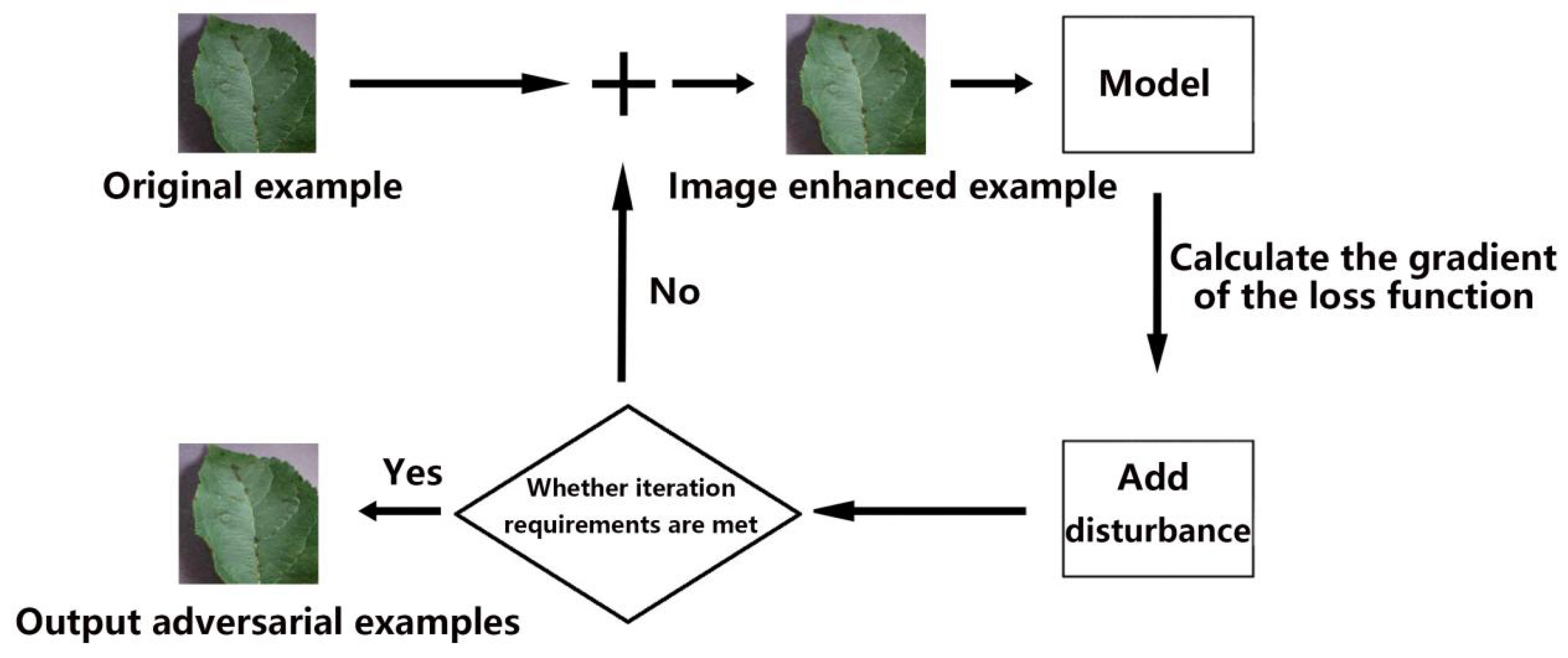
3.3. GP-MI-FGSM
3.3.1. Formulas
3.3.2. Concrete Steps
4. Model Training Strategy
4.1. Learning Rate Decay
4.2. Momentum
4.3. Weight Decay
4.4. Transfer Learning
5. Experimental Results and Analysis
5.1. Classification
5.1.1. Experimental Environment and Parameter Settings
5.1.2. Experimental Data Source
5.1.3. Performance Metrics
5.1.4. Results
5.2. Experiment of Adversarial Example
5.2.1. Experimental Data Source
5.2.2. The Benchmark Method
5.2.3. Hyperparameter Settings
5.2.4. Experimental Results
6. Conclusions
- Compared with VGG16, ResNet50, DenseNet, and EfficientNet, the recognition accuracy of SimAM-EfficientNetB0 is the highest, reaching 99.47%. It has only 3.83 M parameters and takes an average of 1.08 seconds to test a single image, slightly better than DenseNet121 and other models. Ten thousand adversarial examples generated by GP-MI-FGSM were added to the training set. After pretraining and adversarial training, the accuracy of SimAM-EfficientNetB0 reached 99.78%;
- The GP-MI-FGSM adversarial attack algorithm has two advantages in the experiment. Its attack success rate is higher than FGSM, I-FGSM, and MI-FGSM, and the perturbation is too small to be detected by human eyes.
Author Contributions
Funding
Institutional Review Board Statement
Informed Consent Statement
Data Availability Statement
Conflicts of Interest
References
- Crr, C.; Psa, A.; Mea, A.; Fn, B. Identification and recognition of rice diseases and pests using convolutional neural networks-sciencedirect. Biosyst. Eng. 2020, 194, 112–120. [Google Scholar]
- He, K.; Zhang, X.; Ren, S.; Sun, J. Deep residual learning for image recognition. In Proceedings of the International Conference on Computer Vision and Pattern Recognition, Las Vegas, NV, USA, 27–30 June 2016. [Google Scholar]
- Simonyan, K.; Zisserman, A. Very Deep Convolutional Networks for Large-Scale Image Recognition. arXiv 2015, arXiv:1409.1556. [Google Scholar]
- Huang, G.; Liu, Z.; Weinberger, K.Q. Densely connected Cconvolutional networks. In Proceedings of the 2017 IEEE Conference on Computer Vision and Pattern Recognition (CVPR), Honolulu, HI, USA, 21–26 July 2017; pp. 2261–2269. [Google Scholar]
- Durmus, H.; Gunes, E.O.; Kirci, M. A hybrid approach for noise reduction-based optimal classifier using genetic algorithm: A case study in plant disease prediction. In Proceedings of the 2017 6th International Conference on Agro-Geoinformatics, Fairfax, VA, USA, 7–10 August 2017; pp. 1–5. [Google Scholar]
- Iandola, F.N.; Moskewicz, M.W.; Ashraf, K.; Han, S.; Dally, W.J.; Keutzer, K. SqueezeNet: AlexNet-level accuracy with 50x fewer parameters and <1MB model size. arXiv 2016, arXiv:1602.07360. [Google Scholar]
- Zhang, S.W.; Kong, W.W.; Wang, Z. Plant classification method based on dictionary learning with sparse representation. Acta Agric. Zhejiangensis 2017, 29, 338–344. [Google Scholar]
- Guadarrama, L.; Paredes, C.; Mercado, O. Plant Disease Diagnosis in the Visible Spectrum. Appl. Sci. 2022, 12, 2199. [Google Scholar] [CrossRef]
- Kaur, M.; Bhatia, R. Development of an improved tomato leaf disease detection and classification method. In Proceedings of the 2019 IEEE Conference on Information and Communication Technology (CICT), Jeju, Republic of Korea, 6–18 October 2019; pp. 1–5. [Google Scholar]
- Tang, W.; Huang, Z. Lightweight model of tomato leaf diseases identification based on knowledge distillation. Jiangsu J. Agric. Sci. 2021, 37, 9. [Google Scholar]
- Yang, L.; Zhang, R.Y.; Li, L.; Xie, X. Simam: A simple, parameter-free attention module for convolutional neural networks. In Proceedings of the International Conference on Machine Learning PMLR, Virtual, 18–24 July 2021; pp. 11863–11874. [Google Scholar]
- Tan, M.; Le, Q.V. EfficientNet: Rethinking model scaling for convolutional neural networks. In Proceedings of the International Conference on Machine Learning, PMLR, Long Beach, CA, USA, 9–15 June 2019; pp. 6105–6114. [Google Scholar]
- Goodfellow, I.J.; Shlens, J.; Szegedy, C. Explaining and Harnessing Adversarial Examples. arXiv 2019, arXiv:1412.6572. [Google Scholar]
- Moosavi-Dezfooli, S.; Fawzi, A.; Frossard, P. DeepFool: A simple and accurate method to fool deep neural networks. In Proceedings of the 2016 IEEE Conference on Computer Vision and Pattern Recognition (CVPR), Las Vegas, NV, USA, 27–30 June 2016; pp. 2574–2582. [Google Scholar]
- Papernot, N.; Mcdaniel, P.; Jha, S.; Fredrikson, M.; Celik, Z.B.; Swami, A. The limitations of deep learning in adversarial settings. In Proceedings of the 2016 IEEE European Symposium on Security and Privacy (EuroS&P), Saarbrucken, Germany, 21–24 March 2016; pp. 372–387. [Google Scholar]
- Carlini, N.; Wagner, D.A. Towards evaluating the robustness of neural networks. In Proceedings of the 2017 IEEE Symposium on Security and Privacy (SP), San Jose, CA, USA, 22–26 May 2017; pp. 39–57. [Google Scholar]
- Huang, S.; Papernot, N.; Goodfellow, I.; Duan, Y.; Abbeel, P. Adversarial attacks on neural network policies. arXiv 2017, arXiv:1702.02284. [Google Scholar]
- Zhou, D. Universality of Deep Convolutional Neural Networks. arXiv 2020, arXiv:1805.10769. [Google Scholar] [CrossRef]
- O’Shea, K.; Nash, R. An introduction to convolutional neural networks. arXiv 2015, arXiv:1511.08458. [Google Scholar]
- Golhani, K.; Balasundram, S.K.; Vadamalai, G.; Pradhan, B. A review of neural networks in plant disease detection using hyperspectral data. Inf. Process. Agric. 2018, 5, 354–371. [Google Scholar] [CrossRef]
- Toda, Y.; Okura, F. How convolutional neural networks diagnose plant disease. Plant Phenomics 2019, 2019, 9237136. [Google Scholar] [CrossRef] [PubMed]
- Chen, W.; Chen, J.; Duan, R.; Fang, Y.; Ruan, Q.; Zhang, D. MS-DNet: A mobile neural network for plant disease identification. Comput. Electron. Agric. 2022, 199, 107175. [Google Scholar] [CrossRef]
- Hu, J.; Shen, L.; Albanie, S.; Sun, G.; Wu, E. Squeeze-and-Excitation Networks. IEEE Trans. Pattern Anal. Mach. Intell. 2020, 2, 2011–2023. [Google Scholar] [CrossRef] [PubMed]
- Woo, S.; Park, J.; Lee, J.Y.; Kweon, I.S. Cbam: Convolutional block attention module. In Proceedings of the European Conference on 414 Computer Vision (ECCV), Munich, Germany, 8–14 September 2018; pp. 3–19. [Google Scholar]
- Guo, C.; Gardner, J.; You, Y.; Wilson, A.G.; Weinberger, K. Simple black-box adversarial attacks. In Proceedings of the International Conference on Machine Learning, Zhuhai, China, 22–24 February 2019; pp. 2484–2493. [Google Scholar]
- Croce, F.; Hein, M. Sparse and imperceivable adversarial attacks. In Proceedings of the IEEE/CVF International Conference on Computer Vision, Seoul, Republic of Korea, 27 October–2 November 2019; pp. 4724–4732. [Google Scholar]
- Ruder, S. An overview of gradient descent optimization algorithms. arXiv 2016, arXiv:1609.04747. [Google Scholar]
- Robbins, H.E. A Stochastic Approximation Method. Ann. Math. Stat. 2007, 22, 400–407. [Google Scholar] [CrossRef]
- Yosinski, J.; Clune, J.; Bengio, Y.; Lipson, H. How transferable are features in deep neural networks? arXiv 2014, arXiv:1411.1792. [Google Scholar]


| Stage | Operator | Channels | Layers | Resolution |
|---|---|---|---|---|
| 1 | Conv3 × 3 | 32 | 1 | 224 × 224 |
| 2 | MBConv1,k3 × 3 | 16 | 1 | 112 × 112 |
| 3 | MBConv6,k3 × 3 | 24 | 2 | 112 × 112 |
| 4 | MBConv6,k5 × 5 | 40 | 2 | 56 × 56 |
| 5 | MBConv6,k3 × 3 | 80 | 3 | 28 × 28 |
| 6 | MBConv6,k5 × 5 | 112 | 3 | 14 × 14 |
| 7 | MBConv6,k5 × 5 | 192 | 4 | 14 × 14 |
| 8 | MBConv6,k3 × 3 | 320 | 1 | 7 × 7 |
| 9 | Conv1 × 1 & Pooling & FC | 1280 | 1 | 7 × 7 |
| Model | Avg Acc (%) | Avg Sen (%) | Avg Spe (%) | Avg Pre (%) | Time per Epoch (s) | Parameters (M) | Time Cost (s) |
|---|---|---|---|---|---|---|---|
| SimAM-EfficientNetB0 | 99.31% | 97.92% | 99.61% | 98.29% | 642 | 3.83 M | 1.12 |
| SimAM-EfficientNetB1 | 98.32% | 96.11% | 99.35% | 96.11% | 980 | 6.22 M | 1.18 |
| SimAM-EfficientNetB2 | 98.29% | 96.72% | 99.41% | 96.25% | 991 | 8.31 M | 1.21 |
| SimAM-EfficientNetB3 | 98.29% | 96.77% | 99.81% | 96.39% | 1190 | 10.22 M | 1.25 |
| SimAM-EfficientNetB4 | 99.22% | 96.82% | 99.33% | 97.31% | 1680 | 16.75 M | 1.28 |
| SimAM-EfficientNetB5 | 99.15% | 97.11% | 99.28% | 96.77% | 2270 | 27.05 M | 1.42 |
| SimAM-EfficientNetB6 | 99.27% | 95.16% | 99.39% | 96.38% | 2880 | 38.87 M | 1.58 |
| SimAM-EfficientNetB7 | 99.31% | 96.88% | 99.20% | 95.22% | 3580 | 60.86 M | 1.66 |
| SimAM-EfficientNetB0 (pretrained) | 99.47% | 98.11% | 99.89% | 98.78% | 642 | 3.83 M | 1.12 |
| ResNet18 | 98.31% | 93.54% | 99.32% | 96.45% | 1150 | 11.2 M | 1.14 |
| ResNet50 | 98.33% | 95.49% | 99.84% | 95.31% | 1780 | 23.5 M | 1.28 |
| VGG16 | 98.51% | 94.21% | 99.25% | 96.77% | 2880 | 134.4 M | 1.68 |
| DenseNet121 | 98.90% | 97.87% | 99.71% | 97.92% | 1560 | 6.9 M | 1.25 |
| EfficientNetB0 | 99.06% | 96.81% | 99.77% | 97.29% | 642 | 3.83 M | 1.12 |
| Class | TP | TN | FP | FN | Acc (%) | Sen (%) | Spe (%) | Pre (%) |
|---|---|---|---|---|---|---|---|---|
| Apple scab | 50 | 1900 | 0 | 0 | 100 | 100 | 100 | 100 |
| Apple Black rot | 50 | 1900 | 0 | 0 | 100 | 100 | 100 | 100 |
| Apple Cedar apple rust | 50 | 1900 | 0 | 0 | 100 | 100 | 100 | 100 |
| Apple healthy | 50 | 1900 | 0 | 0 | 100 | 100 | 100 | 100 |
| Background without leaves | 50 | 1900 | 0 | 0 | 100 | 100 | 100 | 100 |
| Blueberry healthy | 50 | 1900 | 0 | 0 | 100 | 100 | 100 | 100 |
| Cherry Powdery mildew | 50 | 1900 | 0 | 0 | 100 | 100 | 100 | 100 |
| Cherry healthy | 50 | 1900 | 0 | 0 | 100 | 100 | 100 | 100 |
| Corn Cercospora leaf spot Gray leaf spot | 50 | 1898 | 2 | 0 | 99.9 | 100 | 99.89 | 96.15 |
| Corn Common rust | 50 | 1900 | 0 | 0 | 100 | 100 | 100 | 100 |
| Corn Northern Leaf Blight | 50 | 1900 | 0 | 0 | 100 | 100 | 100 | 100 |
| Corn healthy | 50 | 1900 | 0 | 0 | 100 | 100 | 100 | 100 |
| Grape Black rot | 50 | 1900 | 0 | 0 | 100 | 100 | 100 | 100 |
| Grape Esca (Black Measles) | 50 | 1900 | 0 | 0 | 100 | 100 | 100 | 100 |
| Grape Leaf blight | 50 | 1900 | 0 | 0 | 100 | 100 | 100 | 100 |
| Grape healthy | 50 | 1900 | 0 | 0 | 100 | 100 | 100 | 100 |
| Orange Haunglongbing | 50 | 1900 | 0 | 0 | 100 | 100 | 100 | 100 |
| Peach Bacterial spot | 50 | 1898 | 2 | 0 | 99.9 | 100 | 99.89 | 96.15 |
| Peach healthy | 50 | 1900 | 0 | 0 | 100 | 100 | 100 | 100 |
| Pepper, bell Bacterial spot | 50 | 1900 | 0 | 0 | 100 | 100 | 100 | 100 |
| Pepper, bell healthy | 50 | 1900 | 0 | 0 | 100 | 100 | 100 | 100 |
| Potato Early blight | 49 | 1899 | 0 | 1 | 99.95 | 98 | 100 | 100 |
| Potato Late blight | 49 | 1899 | 0 | 1 | 99.95 | 98 | 100 | 100 |
| Potato healthy | 50 | 1900 | 0 | 0 | 100 | 100 | 100 | 100 |
| Raspberry healthy | 50 | 1900 | 0 | 0 | 100 | 100 | 100 | 100 |
| Soybean healthy | 50 | 1900 | 0 | 0 | 100 | 100 | 100 | 100 |
| Squash Powdery mildew | 50 | 1900 | 0 | 0 | 100 | 100 | 100 | 100 |
| Strawberry Leaf scorch | 50 | 1900 | 0 | 0 | 100 | 100 | 100 | 100 |
| Strawberry healthy | 50 | 1900 | 0 | 0 | 100 | 100 | 100 | 100 |
| Tomato Bacterial spot | 50 | 1900 | 0 | 0 | 100 | 100 | 100 | 100 |
| Tomato Early blight | 49 | 1899 | 0 | 1 | 99.95 | 98 | 100 | 100 |
| Tomato Late blight | 50 | 1900 | 0 | 0 | 100 | 100 | 100 | 100 |
| Tomato Leaf Mold | 50 | 1900 | 0 | 0 | 100 | 100 | 100 | 100 |
| Tomato Septoria leaf spot | 50 | 1898 | 2 | 0 | 99.9 | 100 | 99.89 | 96.15 |
| Tomato mites | 50 | 1900 | 0 | 0 | 100 | 100 | 100 | 100 |
| Tomato Target Spot | 50 | 1900 | 0 | 0 | 100 | 100 | 100 | 100 |
| Tomato Leaf Curl Virus | 50 | 1900 | 0 | 0 | 100 | 100 | 100 | 100 |
| Tomato mosaic virus | 50 | 1900 | 0 | 0 | 100 | 100 | 100 | 100 |
| Tomato healthy | 50 | 1900 | 0 | 0 | 100 | 100 | 100 | 100 |
| Algorithms | VGG16 | ResNet50 | DenseNet | EfficientNet | SimAM-EfficientNetB0 |
|---|---|---|---|---|---|
| FGSM | 92.5% | 88.1% | 87.2% | 86.9% | 86.5% |
| I-FGSM | 92.6% | 89.3% | 88.5% | 87.8% | 86.8% |
| MI-FGSM | 93.1% | 90.2% | 89.9% | 89.3% | 88.7% |
| GP-MI-FGSM | 99.2% | 97.1% | 95.3% | 92.1% | 90.6% |
| Models | mAP (%) | mAP (%) (Slow) | mAP (%) (Medium) | mAP (%) (Fast) |
|---|---|---|---|---|
| SimAM-EfficientNetB0 (adversarial trained) | 99.59% | 98.22% | 99.83% | 98.59% |
| SimAM-EfficientNetB0 (adversarial trained and pretrained) | 99.78% | 99.05% | 99.98% | 99.52% |
| ResNet18 (adversarial trained) | 98.63% | 93.74% | 99.61% | 96.71% |
| ResNet50 (adversarial trained) | 98.61% | 95.72% | 99.87% | 95.73% |
| VGG16 (adversarial trained) | 98.72% | 94.63% | 99.66% | 96.93% |
| DenseNet121 (adversarial trained) | 99.28% | 98.15% | 99.82% | 98.24% |
| EfficientNetB0 (adversarial trained) | 99.32% | 97.21% | 99.89% | 97.79% |
Disclaimer/Publisher’s Note: The statements, opinions and data contained in all publications are solely those of the individual author(s) and contributor(s) and not of MDPI and/or the editor(s). MDPI and/or the editor(s) disclaim responsibility for any injury to people or property resulting from any ideas, methods, instructions or products referred to in the content. |
© 2023 by the authors. Licensee MDPI, Basel, Switzerland. This article is an open access article distributed under the terms and conditions of the Creative Commons Attribution (CC BY) license (https://creativecommons.org/licenses/by/4.0/).
Share and Cite
You, H.; Lu, Y.; Tang, H. Plant Disease Classification and Adversarial Attack Using SimAM-EfficientNet and GP-MI-FGSM. Sustainability 2023, 15, 1233. https://doi.org/10.3390/su15021233
You H, Lu Y, Tang H. Plant Disease Classification and Adversarial Attack Using SimAM-EfficientNet and GP-MI-FGSM. Sustainability. 2023; 15(2):1233. https://doi.org/10.3390/su15021233
Chicago/Turabian StyleYou, Haotian, Yufang Lu, and Haihua Tang. 2023. "Plant Disease Classification and Adversarial Attack Using SimAM-EfficientNet and GP-MI-FGSM" Sustainability 15, no. 2: 1233. https://doi.org/10.3390/su15021233
APA StyleYou, H., Lu, Y., & Tang, H. (2023). Plant Disease Classification and Adversarial Attack Using SimAM-EfficientNet and GP-MI-FGSM. Sustainability, 15(2), 1233. https://doi.org/10.3390/su15021233