SCDNet: Self-Calibrating Depth Network with Soft-Edge Reconstruction for Low-Light Image Enhancement

Abstract

Captured low-light images typically suffer from low brightness, low contrast, and blurred details due to the scattering and absorption of light and limited lighting. To deal with these issues, we propose a self-calibrating depth network with soft-edge reconstruction for low-light image enhancement. Concretely, we first employ the soft edge reconstruction module to reconstruct the soft edge of the input image and extract the texture and detail information of the image. Afterward, we explore the convergence properties of each input via the self-calibration module to significantly improve the computational effectiveness of the method and gradually correct the inputs at each subsequent level. Finally, the low-light image is iteratively enhanced by an iterative light enhancement curve to obtain a high-quality image. Extensive experiments demonstrate that our SCDNet visually enhances the brightness and contrast, restores the actual color, and makes the image more in line with the characteristics of the human eye vision system. Meanwhile, our SCDNet outperforms the compared methods in some qualitative and quantitative metrics.

1. Introduction

With the development of science and technology, photographic equipment is becoming increasingly developed, and people’s requirements for image quality are getting higher and higher. Still, due to the influence of environmental factors, people often cannot take the right images. Additionally, often, because of the effect of backlight, uneven lighting, and low lighting, the acquisition of image information is not perfect, thereby reducing the quality of the image. Not only everyday images but other industries that require image quality, such as intelligent transportation, visual surveillance, etc., expect a high-quality image, so the quality enhancement of images is worth exploring [1,2,3]. In recent years, low-light image enhancement techniques can be roughly divided into three types: image-based enhancement, image-based restoration, and deep learning-based. Among them, deep learning-based image enhancement methods are developing particularly rapidly [4,5,6,7].

Image enhancement-based methods: Image enhancement methods generally achieve the purpose of enhancing images by directly modifying the pixel value distribution of the image [8], such as histogram equalization and other methods. Voronin et al. [9] proposed a new thermal image enhancement algorithm based on local and regional frequency domain processing, which performs log-transformed histogram match and spatial equalization on different image blocks. UEDA et al. [10] proposed a method for image enhancement of a single backlit image using histogram specifications, identifying the target shape of an intensity histogram that improves the bimodal distribution, and then performing intensity conversion through histogram specifications while maintaining hue and saturation. Pugazhenthi et al. [11] proposed a bi-Histogram Equalization based on bi-histogram equilibrium, the automatic histogram equalization algorithm, which applies image brightness normalization to reduce the absolute average brightness error. Kong et al. [12] proposed a Poisson noise-aware Retinex model, which, for the first time considered using a Poisson distribution to define the fidelity term driven by Retinex, and construct Poisson noise distribution a priori to achieve suppression and successfully realize the retention of image structure information while removing noise. Xu et al. [13] constructed a Retinex model of structural and texture perception to distinguish between light and reflection gradients. The closed-form solution of the two target variables is derived by alternating optimization and vectorization of least squares techniques. Hao et al. [14] proposed a Gaussian full-variational model for Retinex decomposition in a semi-decoupled manner for increasing brightness and suppressing noise simultaneously.

Image reproduction-based methods: Image restoration methods include using various filters to directly change the blur [15], distortion, and noise of the image. Cai et al. [16] designed a combined intrinsic and extrinsic a priori model to observe the illumination and reflectivity of images, a method that preserves structural information through shape prior, but there is insufficient enhancement. Ren et al. [17] proposed a low-light image enhancement framework that uses the response characteristics of the camera to adjust each pixel to the appropriate exposure based on the estimated exposure rate map by combining exposure estimates of exposures for illumination. To solve the overexposure phenomenon of the low-light image enhancement method, Zhang et al. [18] introduced a series of lighting constraints from different angles. They regarded the exposure correction problem as a light estimation optimization to produce the expected results with constant exposure, vivid colors, and sharp textures. Still, too many constraints make the algorithm solution cumbersome, resulting in significantly slower inference.

Based on deep learning: Deep learning is now widely used in a variety of vision processing [19,20,21], and its ease and speed in handling charges are very popular. Shen et al. [22] combined convolutional neural networks with Retinex theory to equate feed-forward convolutional neural networks with different Gaussian convolutional nuclei to multiscale Retinex, Thus, a multi-scale convolutional neural network MSR-net (Multi-scale Retinex network) is designed, and the end-to-end mapping between low-light images and normal brightness images is directly learned, and end-to-end low-light image enhancement network is obtained. Li et al. [23] proposed a trainable convolutional neural network for low-light image enhancement. They trained the network structure of the design by taking a low-light image as input and outputting its lightmap, which was then used to obtain enhanced images based on the Retinex model. While this method can achieve satisfactory enhancements on some images, there are still bad results on some challenging real-world scenes. Ren et al. [24] designed a hybrid network of two different streams that could learn both global content and clear images in a unified network to restore more accurate scene content. However, due to the problem of encoders, this method often causes the problem of loss of structural details. Tao et al. [25] proposed a low-light CNN-based learning framework, which utilizes multiscale feature maps to avoid the gradient disappearance problem, and uses SSIM loss to train the model to preserve image texture, thereby adaptively enhancing the low contrast of the light image. Lore et al. [26] used a depth autoencoder called Low-Light Net (LLNet) to perform contrast enhancement and denoising. Yang et al. [27] experimented with semi-supervised learning with low-light image enhancement. In this work, a deep recursive band representation is established to connect fully supervised and unsupervised learning frameworks and combine their strengths. In general, the advantages of deep learning methods over other methods are relatively obvious [28,29,30,31].

Overall, existing methods can improve the quality of images to some extent, but there are still some issues that are worth improving, such as insufficient enhancement, color distortion, and loss of detail. To further improve the image quality, a new low-light image enhancement method is proposed based on the self-calibration depth curve estimation of soft-edge reconstruction. Experimental results show that the proposed method has the advantages of the light network, low time consumption, and obvious enhancement effect. We summarize our contribution as follows:

(1)

We propose a self-calibrated iterative image enhancement method based on soft edge reconstruction. This method first softens the input image and then extracts the feature details, then the self-calibration module accelerates the convergence of the input and feeds it into the enhancement network, and finally iteratively enhances the low-light image according to the gloss curve to obtain a high-quality image. This method can not only better extract image details, but also accelerate the convergence speed of the network, making the output more efficient and stable.

(2)

For low-light image texture loss and detail blur, we introduce a soft edge reconstruction module to detect image features at different scales, extracting clear and sharp edge features of the image through the softening extraction of image edges and the reconstruction of image details.

(3)

This paper ensures exposure stability of the input image by introducing a self-calibration module to perform stepwise convergence of the image. Lightweight networks can significantly improve computational efficiency, thereby accelerating network convergence, which enhances image quality while reducing processing speed.

2. Proposed Method

2.1. Network Model

This paper proposes a self-calibration depth curve estimation network based on soft-edge reconstruction, and the net framework schematic is shown in Figure 1. After the original image is fed, the soft edge reconstruction is first performed, the image edge is softened and then upsampled after passing through three multi-scale Residual Blocks (MSRB) and the bottleneck layer to extract the image details, and then the results are fed into the self-calibration module for processing. The self-calibration module converges on the results and improves exposure stability, then learns the processed image of the input, estimates a best-fitting light enhancement curve, and finally iteratively enhances the given input image.

2.2. Soft-Edge Reconstruction Module

Image edge priors are one of the most productive priors, and image edges are essential to image characterization. Many edge-assisted or edge-guided image processing methods have verified the superiority and desirability of image edge prior. However, implementing some methods is more complex and has certain limitations. To this end, a productive Edge-Net is introduced to reconstruct sharp [32], super-resolution soft edges directly from low-quality images. After verification, after directly upsampling the original image, the soft edges of the image are blurry. They have much noise, and the soft edges of the image extracted after the image are reconstructed by the soft edges which are clear and sharp, improving the image texture and detail information.

For Edge-Net, a modified version of the Multi-scale Residual Network (MSRN) is adopted as its structure. MSRN can detect image features at different scales comfortably, which facilitates the extraction of soft edges of subsequent images. Image soft edges preserve a more comprehensive image edge information, which can be expressed as follows:

$$I_{Edge}=div(u_x,u_y),$$

(1)

where $u_i=\frac{{\nabla }_i=I}{\sqrt{1+{\left|\nabla I\right|}^2}}$, $x$ for the horizontal direction and $y$ for the perpendicular direction, $i\in \left\{x,y\right\}$, $\nabla$ represents the gradient operation and $div$ represents the scatter operation. The corresponding soft edges are obtained from the original image, which accurately describes the changes in the gradient domain.

2.3. Self-Calibrated Module

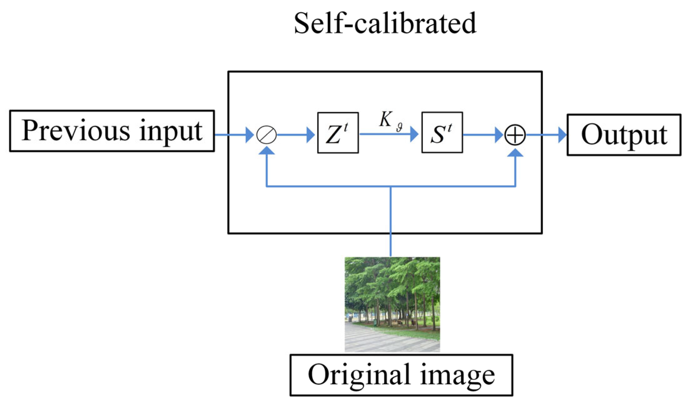
To explore the convergence characteristics of the first stage of the input and each subsequent step, a self-calibrated module was introduced [33]. The self-calibration module converges between results at each location, improving exposure stability and significantly reducing the computational burden and links between outcomes at each acceleration stage. The flow chart of the self-calibration module is shown in Figure 2, where $z^t$ is obtained after the operation of the previous input and the original image. Then, $s^t$ is obtained after the operation of $z^t$ and $K_{\vartheta }$. Finally, $s^t$ is output after the operation of $y$ to complete the self-calibration module.

The self-calibration module constructed in this paper indirectly affects the output of each stage by integrating physical principles and gradually correcting the inputs of each stage, showing the visible results of different settings. It can be seen that this paper can instantiate it with a sufficiently lightweight architecture, and more importantly, the self-calibration module is only used during the training phase. No matter what convolution number is set, the self-calibration module always produces a stable output. The output of the self-calibration module is:

$$g(x^t):\left\{\begin{array}{l}{z}^t=y\oslash x^t\hfill \\ s^t=K_{\vartheta }(z^t)\hfill \\ v^t=y+s^t\hfill \end{array}\right.,$$

(2)

where $y$ is the original image, $t\ge 1$, $x^t$ represents the input of the previous level, $v^t$ represents the output of each stage, $K$ is the introduced parameterization operator, and $\vartheta$ is the parameter with learning function.

2.4. Iteration Module

To rationalize the use of the inputs processed by the first two modules, this paper introduces the Deep Curve Estimation NET (DCE-NET), which automatically maps low-light images to enhancement curves and calculates a best-fit set of light enhancement curves for the input image. The adaptive curve parameters depend entirely on the input image. The framework then maps all pixels of the input RGB channel by iteratively applying curves to achieve the optimal enhanced image. This module can reduce the risk of oversaturation by dropping each pixel value in the normalized range of each pixel value in this module. In addition, this module is simple and can guarantee the contrast difference between adjacent pixels and the brightness of different areas. For the above process, it is used $\mathrm{LE}$ to represent the result of each iteration:

$${\mathrm{LE}}_1=\mathrm{LE}\left(I;A_1\right),$$

(3)

where ${\mathrm{LE}}_1$ represents the result of the first iteration, $I$ is the original input image, $A_1$ represents the RGB channel image after processing from the previous module, using Equation (3), the result of the $N$ th iteration can be further deduced as:

$${\mathrm{LE}}_n=\mathrm{LE}\left({\mathrm{LE}}_{n-1};A_n\right),$$

(4)

where ${\mathrm{LE}}_n$ denotes the result of the $N$ th iteration, ${\mathrm{LE}}_{n-1}$ denotes the result of $N-1$ iterations, and $A_n$ denotes the $N$ th image processed from the previous module after the RGB channel.

2.5. Loss Function

We introduce four types of loss functions to train the network, namely color constancy loss, exposure control loss, spatial consistency loss, and illumination smoothness loss. The overall loss is the additive sum of these four loss functions.

Color constancy loss: Color constancy in the grayscale world assumes that for an image with a large number of color variations, the average of its three RGB channel components converges to the same gray level [34]. Based on this theory, we introduce a color invariance loss to remove the color bias present in the enhanced image and to establish the relationship between the three adjusted channels. The loss $L_{ccl}$ can be expressed as:

$$L_{ccl}={\displaystyle \sum _{\forall (m,n)\in \epsilon }(P^m-P^n{)}^2},\epsilon =\{(R,G),(R,B),(G,B)\},$$

(5)

where $(m,n)$ denotes the color channel and $P^m$ indicates the average value of intensity of channel $m$ in the enhanced image.

Exposure control loss: To suppress underexposed or overexposed areas, exposure control loss $L_{ecl}$ is used to keep exposure levels in check. Exposure control loss gauges the relationship between the average intensity value of a local area and a good exposure level $E$. Li et al. [34] set $E$ as a gray level in RGB color space, and we tested in our experiments that $E$ did not vary much between 0.4 and 0.7, so we set the value of $E$ to 0.55 in our experiments. The loss $L_{ecl}$ can be expressed as:

$$L_{ecl}=\frac{1}{X}{\displaystyle {\sum }_{Z=1}^X\left|J_Z-E\right|},$$

(6)

where $X$ denotes the number of un-overlapping local areas of size 8 × 8, $Z$ is the number of local areas, and $J$ denotes the average strength value of the local areas in the enhanced image.

Spatial consistency loss: Spatial consistency loss promotes the improvement of the spatial consistency of the image by keeping the variance of adjacent regions between the input image and its enhanced image [34]. The loss $L_{s\mathrm{cl}}$ can be expressed as:

$$L_{s\mathrm{cl}}=\frac{1}{Z}{\displaystyle \sum _{i=1}^Z{\displaystyle \sum _{j\in \mathsf{\Omega }(i)}{(\left|(Y_i-Y_j)\right|-\left|(I_i-I_j)\right|)}^2}},$$

(7)

where $\mathsf{\Omega }(i)$ denotes the four adjacent areas (top, bottom, left, right) focused on region $i$. Denote $Y$ and $I$ as the average intensity values in the local area of the enhanced image and the input image, respectively. According to extensive experimental verification, better results are shown when the partial area size is set to 8 × 8.

Illumination smoothness loss: To maintain the relationship of adjacent pixels in monotonicity, light smoothing losses are added to each curve parameter graph [34]. The loss $L_{isl}$ can be expressed as:

$$L_{isl}=\frac{1}{N}{\displaystyle \sum _{n=1}^N{\displaystyle \sum _{c=\xi }^{}(\left|{\nabla }_x{A}_n^c\right|)}}+\left|{\nabla }_y{A}_n^c\right|{)}^2,\xi =\{\mathrm{r},\mathrm{g},\mathrm{b}\},$$

(8)

where $N$ denotes the number of iterations, $\nabla x$ and $\nabla y$ denote horizontal and visual staircase manipulation, respectively.

The overall loss is the weighted sum of all losses and can be expressed as:

$$L=L_{ccl}+L_{ecl}+W_{scl}{L}_{scl}+W_{isl}{L}_{isl},$$

(9)

where $W_{s\mathrm{cl}}$ and $W_{isl}$ are the weights of the corresponding losses, it has been verified that the value of $W_{s\mathrm{cl}}$ is set at 0.5, and the importance of $W_{isl}$ is set at 20 for the best results.

3. Experimental Results

3.1. Experimental Settings

The computer experimented with in this paper is specifically configured as an NVIDIA TeslaV100S with 32 GB of video memory. The software environment is Python 3 under the 64-bit Window10 operating system 7.

To improve the training accuracy of the network, this paper adopts a variety of dataset sequences, integrates multiple exposures and various low-light image data, and more diverse data sets can bring better visual effects. This paper selects SICE [35], DICM [36], LIME [37], VV (https://sites.google.com/site/vonikakis/datasets), and MEF [38] as part of the image data in the composition of 2000 images as a training set. The training data size of this paper is set to 512 × 512, the application batch is 8, and the batch volume is 100. This paper selected 200 images from the LOL [39] low-light dataset as the test set.

In addition, to verify the effectiveness of the proposed method, this paper conducts a large number of experimental analyses on the aspects of subjective visual evaluation and objective evaluation indicators. The proposed method is subjectively and objectively compared with seven traditional methods and three deep learning methods to verify the method’s effectiveness fully. The comparison methods include traditional methods LR3M [40], L2LP [41], BIMEF [42], FBEM [43], FEM [44], LLIE [45], and AIEM [46]; and deep learning-based methods TFFR [33], Zero-DCE [47], and Zero-DCE+ [34]. We run the provided source code by using the recommended parameters to output the best results for the different methods.

3.2. Subjective Evaluation

To verify the advantages of the methods in this document, the methods of this document are compared with various methods. Standard low-light images, global over-dimming images, locally dimmed images, extremely dark images, and locally overexposed images were selected for subjective comparison.

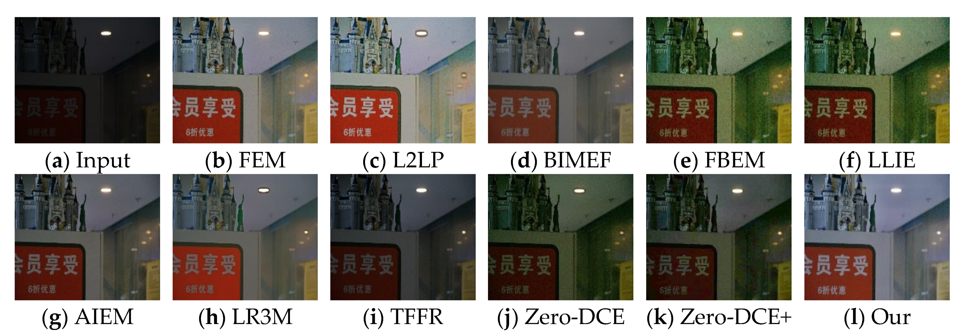
In the standard low-light images, as shown in Figure 3, due to the processing method problem of LR3M [40], and TFFR [33], there is an obvious overexposure occurring in some light areas and sunlight areas, and the problem of over-enhancement occurs. FEM [44], BIMEF [42], and FBEM [43] contrast enhancement is not satisfactory, L2LP [42], Zero-DCE [47], and Zero-DCE+ [34] have an excellent enhancement for low light images, but not as good as our method in terms of detail enhancement. Additionally, our method achieves gratifying results in terms of overall enhancement, exposure and detail enhancement.

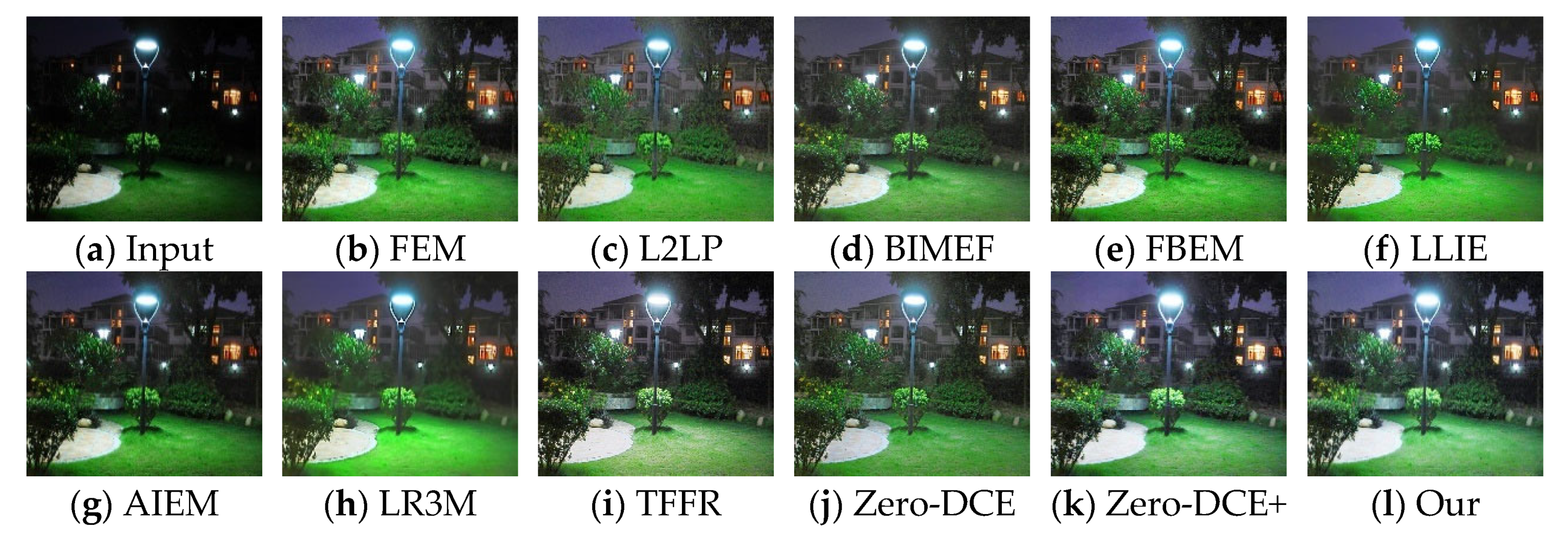
In the global over dark images, as shown in Figure 4, there is color distortion in the method processing of FBEM [43], LLIE [45], Zero-DCE [47], and Zero-DCE+ [34]; BIMEF [43], and TFFR [33] have under-enhancement issues, and while FEM [44], L2LP [41], AIEM [46], and LR3M [40] have better enhancement effects, there are artifacts, blur, and insufficient detail feature extraction in the background lighting. In contrast, our method not only enhances well but also has better results in the extraction of some feature information and texture information.

In the locally over dark images, as shown in Figure 5, FEM [44], L2LP [41], FBEM [43], LLIE [45], and TFFR [33] have serious problems with noise at the lights. AIEM [46], BIMEF [42], and LR3M [40] local areas are too dark, part of the enhancement effect is not obvious, and the detail extraction of too-dark areas is not obvious, while Zero-DCE [47], Zero-DCE+ [34] and our method achieve better results in terms of enhancement and detail extraction.

In the extremely dark images, as shown in Figure 6, FBEM [43], AIEM [46], Zero-DCE [47], and Zero-DCE+ [34] suffer from under-enhancement, in addition to under-extraction of detail information in dark areas. FEM [44], L2LP [41], and FBEM [43] have severe noise. LR3M [40], LLIE [45], and BIMEF [42] have unclear details and blurred textures.

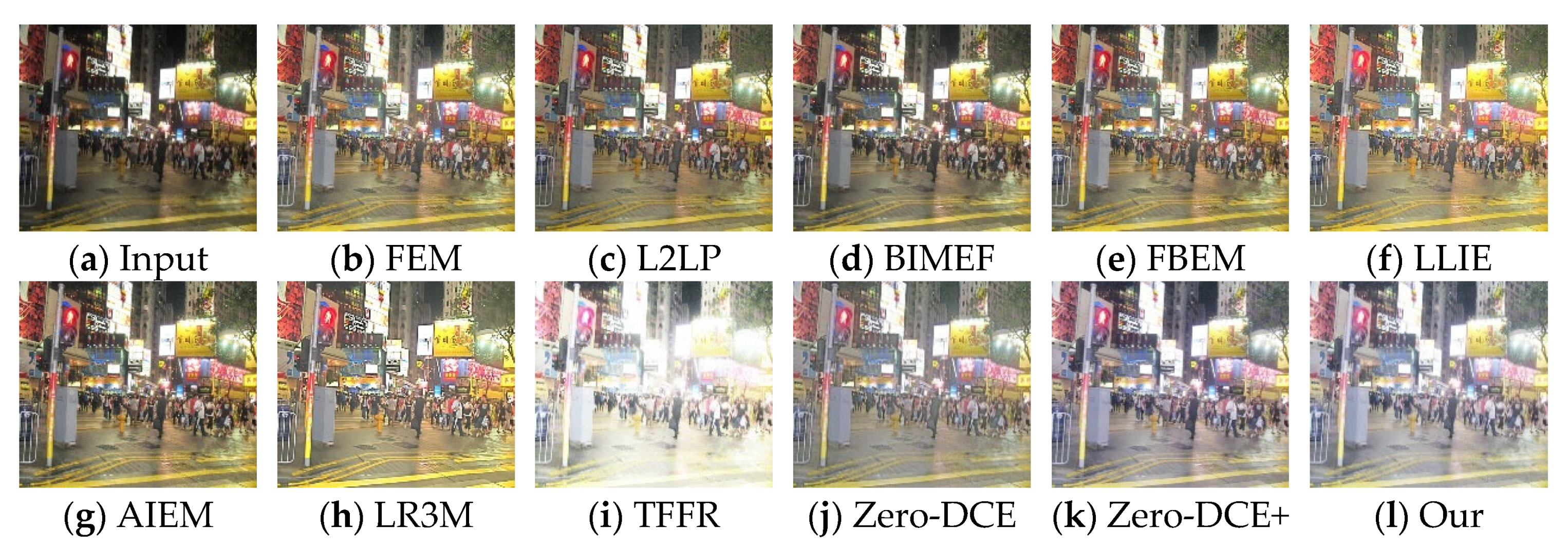
In the locally overexposed images, as shown in Figure 7, there is severe overexposure in TFFR [33] and slight overexposure in Zero-DCE [47], Zero-DCE+ [34] and our method, while our method has significant advantages in feature information extraction and detail information preservation.

3.3. Objective Evaluation

In this paper, several standard methods are selected for objective evaluation, namely information Entropy (IE), peak signal-to-noise ratio (PSNR), structural similarity (SSIM), normalized root mean square error (NRMSE) and root mean square error (RMSE). For example, as shown in

Table 1. Objective evaluation of optimal results of different methods.

Methods	IE ↑	PSNR ↑	SSIM ↑	NRMSE ↓	RMSE ↓
LR3M [40]	6.856	15.316	0.591	1.009	39.215
L2LP [41]	7.325	14.835	0.503	1.012	43.264
BIMEF [42]	7.235	15.635	0.492	1.695	43.586
FEM [44]	7.519	13.876	0.487	2.211	52.367
FBEM [43]	7.232	13.437	0.498	2.024	61.354
LLIE [45]	7.124	14.235	0.506	1.351	47.391
AIEM [46]	7.465	13.987	0.469	2.036	52.367
TFFR [33]	6.754	11.789	0.417	1.975	74.259
Zero-DCE [47]	7.544	13.849	0.478	1.857	52.152
Zero-DCE+ [34]	7.635	12.954	0.389	1.956	59.367
Our	7.873	15.642	0.673	0.360	42.113

, the best result is in red and the second best result is in blue under each case.

As shown in Table 1, the objective evaluation metrics of the optimal result images are derived after we run the LOL [39] public dataset using the parameters recommended by the source code of each method. As can be seen from the objective evaluation in Table 1, compared with the comparative methods, our method obtained the best results in IE, PSNR, SSIM, and NRMSE, and the second-best results in RMSE. As shown by the objective evaluation metrics, our method performs well in the enhancement of low-light images at different quality levels.

As shown in

Table 2. Objective evaluation of different methods.

Methods	IE ↑	PSNR ↑	SSIM ↑	NRMSE ↓	RMSE ↓
LR3M [40]	6.657	14.909	0.531	1.175	44.529
L2LP [41]	6.960	14.083	0.534	1.348	46.694
BIMEF [42]	7.018	15.251	0.460	1.808	45.193
FEM [44]	7.318	13.493	0.404	2.623	57.106
FBEM [43]	7.018	13.232	0.472	2.131	69.154
LLIE [45]	6.966	13.983	0.452	1.877	51.743
AIEM [46]	7.256	13.520	0.395	2.542	58.878
TFFR [33]	6.353	11.089	0.367	2.183	76.629
Zero-DCE [47]	7.104	13.459	0.412	2.003	55.519
Zero-DCE+ [34]	7.152	12.352	0.359	2.274	62.720
Our	7.832	15.194	0.655	0.434	44.840

, the overall resultant image objective evaluation metrics are derived after we ran the LOL [39] public dataset using the parameters recommended by the source code of each method, our method achieves the best results for IE, SSIM, and NRMSE our method, and the second-best results for PSNR and RMSE our method compared with the comparison methods. In summary, our method has good enhanced performance in objective evaluation metrics.

3.4. Ablation Study

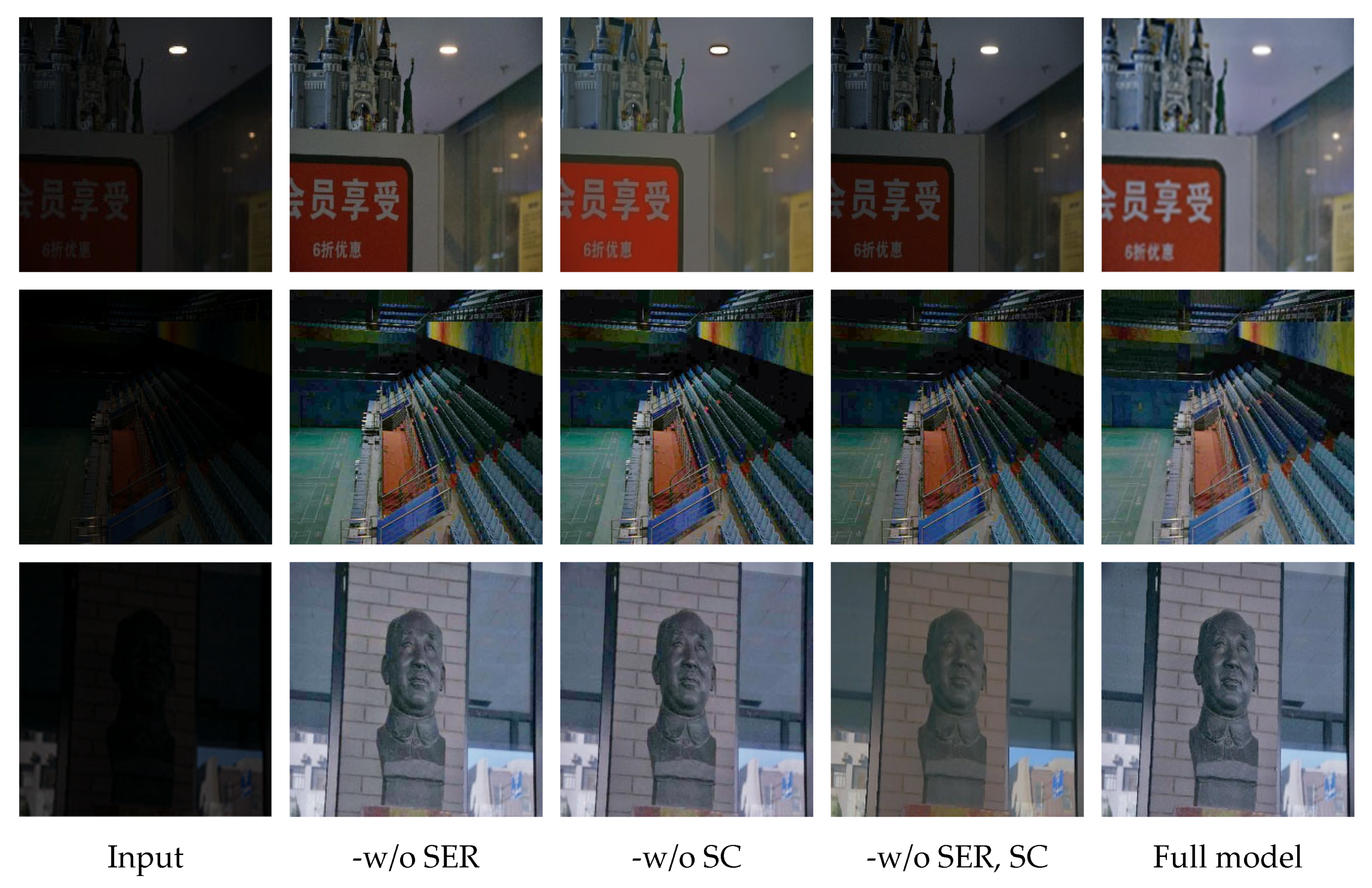
To prove the effectiveness of the various modules of this network, this paper conducts an ablation study. Specifically, (1) our model has no soft edge reconstruction module (-w/o SER), (2) our model has no self-calibration module (-w/o SC), and (3) our model has no soft edge reconstruction module, no self-calibration module (-w/o SER, SC). As shown in

Table 3. Ablation experimental results.

Methods	IE↑	PSNR ↑	SSIM ↑	NRMSE ↓	RMSE ↓
-w/o SER	7.179	11.078	0.321	2.531	72.924
-w/o SC	7.176	10.838	0.313	2.640	74.772
-w/o SER, SC	7.122	11.854	0.341	2.309	66.709
Full model	7.832	15.194	0.655	0.434	44.840

, the verification results are compared after the multiple modules of this method are disassembled and carried out for experiments.

As can be seen from Table 3, the complete network model has superior performance in all aspects when compared to the incomplete network model. The experimental results verify that the simultaneous introduction of software reconstruction and self-calibration still has a large impact on the final results. Although the improvement in information entropy is not much, the performance is improved by about 50% in PSNR, almost doubled in SSIM, and a considerable improvement in normalized root-mean-square error and root-mean-square error is seen. As can be seen from Figure 8, the enhancement effect is significantly worse when both SER and SC modules are not available, and there is a significant improvement in the visual effect with the addition of SER and SC modules. This shows that the soft-edge reconstruction module and the self-calibration module can indeed significantly improve the image details, thus leading to enhanced image enhancement.

In addition to the ablation experiments of the model module, we also conducted ablation experiments of the losses. Specifically, a comparison of the absence of one of the four loss functions and the full loss function, respectively.

As can be seen in

Table 4. Loss ablation experiment results.

Losses	IE↑	PSNR ↑	SSIM ↑	NRMSE ↓	RMSE ↓
$-\mathrm{w}/\mathrm{o} L_{ccl}$	7.514	14.297	0.395	0.725	54.648
$-\mathrm{w}/\mathrm{o} L_{ecl}$	7.431	13.173	0.357	2.516	63.374
$-\mathrm{w}/\mathrm{o} L_{s\mathrm{cl}}$	7.145	12.572	0.403	1.363	46.729
$-\mathrm{w}/\mathrm{o} L_{isl}$	7.334	13.425	0.449	1.373	50.304
$-\mathrm{w}/\mathrm{o} L_{}$ (full loss)	7.832	15.194	0.655	0.434	44.840

, each of our loss functions is critical, and the absence of any one of them leads to less than satisfactory results, with exposure control loss being particularly important; without it, four of our five metrics show poor results.

Finally, we also added a runtime comparison. Since our comparison tests were run on different platforms, we could only run the time comparison on the same computer.

From

Table 5. Running time comparison results.

Methods	Platform	Time	Methods	Platform	Time
LR3M [40]	Matlab	0.579	AIEM [46]	Matlab	0.529
L2LP [41]	Matlab	0.076	TFFR [33]	Python	0.117
BIMEF [42]	Matlab	32.429	Zero-DCE [47]	Python	0.259
FEM [44]	Matlab	3.742	Zero-DCE+ [34]	Python	0.143
FBEM [43]	Matlab	0.246	Our	Python	0.093
LLIE [45]	Matlab	0.932

, although our model borrows from Zero-DCE+ [26], our runtime is even superior due to our addition of the self-calibration module, and our results rank second in overall runtime, which is better than most of the methods.

4. Conclusions

This paper’s efficient low-light image enhancement method relies on a self-calibrated depth curve estimation network for soft-side reconstruction. First, the soft edge reconstruction module is used to reconstruct the edges and details of the input image, extract the more prominent edge features in the image, and ensure that the details and texture information of the result is enhanced. Secondly, the lightweight self-calibration module accelerates the convergence operation of each input image. It iteratively enhances the input image through the iterative enhancement curve, thereby improving the enhanced quality of the low-light image. Enhancement experiments on various low-light images show that the proposed method has achieved apparent visual effects in detail enhancement and color reproduction and is superior to other similar methods.

Although the method in this paper has achieved positive results in a large number of experiments and has certain advantages in processing speed, it still has some shortcomings. First of all, although the proposed method is efficient, it still has poor results for some specific image processing; secondly, although our model is exposure-stabilized in the self-calibration module, it still suffers from overexposure after processing in some specific scenes (e.g., sky, etc.). In future work, the focus will be on addressing these issues.

References

1. Hu, Z.; Yin, Z.; Qin, L.; Xu, F. A Novel Method of Fault Diagnosis for Injection Molding Systems Based on Improved VGG16 and Machine Vision. Sustainability 2022, 14, 14280. [Google Scholar] [CrossRef]
2. Zhang, W.; Wang, Y.; Li, C. Underwater Image Enhancement by Attenuated Color Channel Correction and Detail Preserved Contrast Enhancement. IEEE J. Ocean. Eng. 2022, 47, 718–735. [Google Scholar] [CrossRef]
3. Liu, Y.; Yan, Z.; Tan, J.; Li, Y. Multi-Purpose Oriented Single Nighttime Image Haze Removal Based on Unified Variational Retinex Model. IEEE Trans. Circuits Syst. Video Technol. 2022. [Google Scholar] [CrossRef]
4. Li, J.; Zhang, X.; Feng, P. Detection Method of End-of-Life Mobile Phone Components Based on Image Processing. Sustainability 2022, 14, 12915. [Google Scholar] [CrossRef]
5. Qi, Q.; Li, K.; Zheng, H.; Gao, X.; Hou, G.; Sun, K. SGUIE-Net: Semantic Attention Guided Underwater Image Enhancement with Multi-Scale Perception. IEEE Trans. Image Process. 2022, 31, 6816–6830. [Google Scholar] [CrossRef] [PubMed]
6. Zhang, W.; Dong, L.; Xu, W. Retinex-Inspired Color Correction and Detail Preserved Fusion for Underwater Image Enhancement. Comput. Electron. Agric. 2022, 192, 106585. [Google Scholar] [CrossRef]
7. Zhang, W.; Dong, L.; Zhang, T.; Xu, W. Enhancing Underwater Image via Color Correction and Bi-Interval Contrast Enhancement. Signal Process. Image Commun. 2021, 90, 116030. [Google Scholar] [CrossRef]
8. Chen, L.; Zhang, S.; Wang, H.; Ma, P.; Ma, Z.; Duan, G. Deep USRNet Reconstruction Method Based on Combined Attention Mechanism. Sustainability 2022, 14, 14151. [Google Scholar] [CrossRef]
9. Voronin, V.; Tokareva, S.; Semenishchev, E.; Agaian, S. Thermal Image Enhancement Algorithm Using Local and Global Logarithmic Transform Histogram Matching with Spatial Equalization. In Proceedings of the 2018 IEEE Southwest Symposium on Image Analysis and Interpretation (SSIAI), Las Vegas, NV, USA, 8–10 April 2018; pp. 5–8. [Google Scholar]
10. Ueda, Y.; Moriyama, D.; Koga, T.; Suetake, N. Histogram Specification-Based Image Enhancement for Backlit Image. In Proceedings of the 2020 IEEE International Conference on Image Processing (ICIP), Abu Dhabi, United Arab Emirates, 25–28 October 2020; pp. 958–962. [Google Scholar]
11. Pugazhenthi, A.; Kumar, L.S. Image Contrast Enhancement by Automatic Multi-Histogram Equalization for Satellite Images. In Proceedings of the 2017 Fourth International Conference on Signal Processing, Communication and Networking (ICSCN), Chennai, India, 16–18 March 2017; pp. 1–4. [Google Scholar]
12. Kong, X.-Y.; Liu, L.; Qian, Y.-S. Low-Light Image Enhancement via Poisson Noise Aware Retinex Model. IEEE Signal Process. Lett. 2021, 28, 1540–1544. [Google Scholar] [CrossRef]
13. Xu, J.; Hou, Y.; Ren, D.; Liu, L.; Zhu, F.; Yu, M.; Wang, H.; Shao, L. Star: A Structure and Texture Aware Retinex Model. IEEE Trans. Image Process. 2020, 29, 5022–5037. [Google Scholar] [CrossRef]
14. Hao, S.; Han, X.; Guo, Y.; Xu, X.; Wang, M. Low-Light Image Enhancement with Semi-Decoupled Decomposition. IEEE Trans. Multimed. 2020, 22, 3025–3038. [Google Scholar] [CrossRef]
15. Zhang, Z.; Su, Z.; Song, W.; Ning, K. Global Attention Super-Resolution Algorithm for Nature Image Edge Enhancement. Sustainability 2022, 14, 13865. [Google Scholar] [CrossRef]
16. Cai, B.; Xu, X.; Guo, K.; Jia, K.; Hu, B.; Tao, D. A Joint Intrinsic-Extrinsic Prior Model for Retinex. In Proceedings of the IEEE International Conference on Computer Vision, Venice, Italy, 22–29 October 2017; pp. 4000–4009. [Google Scholar]
17. Ren, Y.; Ying, Z.; Li, T.H.; Li, G. LECARM: Low-Light Image Enhancement Using the Camera Response Model. IEEE Trans. Circuits Syst. Video Technol. 2018, 29, 968–981. [Google Scholar] [CrossRef]
18. Zhang, Q.; Yuan, G.; Xiao, C.; Zhu, L.; Zheng, W.-S. High-Quality Exposure Correction of Underexposed Photos. In Proceedings of the 26th ACM International Conference on Multimedia, Seoul, Republic of Korea, 22–26 October 2018; pp. 582–590. [Google Scholar]
19. Mariani, P.; Quincoces, I.; Haugholt, K.H.; Chardard, Y.; Visser, A.W.; Yates, C.; Piccinno, G.; Reali, G.; Risholm, P.; Thielemann, J.T. Range-Gated Imaging System for Underwater Monitoring in Ocean Environment. Sustainability 2018, 11, 162. [Google Scholar] [CrossRef] [Green Version]
20. Shen, L.; Yue, Z.; Feng, F.; Chen, Q.; Liu, S.; Ma, J. Msr-Net: Low-Light Image Enhancement Using Deep Convolutional Network. arXiv 2017, arXiv:1711.02488. [Google Scholar]
21. Guo, H.; Lu, T.; Wu, Y. Dynamic Low-Light Image Enhancement for Object Detection via End-to-End Training. In Proceedings of the 2020 25th International Conference on Pattern Recognition (ICPR), Milan, Italy, 10–15 January 2021; pp. 5611–5618. [Google Scholar]
22. Al Sobbahi, R.; Tekli, J. Low-Light Homomorphic Filtering Network for Integrating Image Enhancement and Classification. Signal Process. Image Commun. 2022, 100, 116527. [Google Scholar] [CrossRef]
23. Li, C.; Guo, J.; Porikli, F.; Pang, Y. LightenNet: A Convolutional Neural Network for Weakly Illuminated Image Enhancement. Pattern Recognit. Lett. 2018, 104, 15–22. [Google Scholar] [CrossRef]
24. Ren, W.; Liu, S.; Ma, L.; Xu, Q.; Xu, X.; Cao, X.; Du, J.; Yang, M.-H. Low-Light Image Enhancement via a Deep Hybrid Network. IEEE Trans. Image Process. 2019, 28, 4364–4375. [Google Scholar] [CrossRef]
25. Tao, L.; Zhu, C.; Xiang, G.; Li, Y.; Jia, H.; Xie, X. LLCNN: A Convolutional Neural Network for Low-Light Image Enhancement. In Proceedings of the 2017 IEEE Visual Communications and Image Processing (VCIP), St. Petersburg, FL, USA, 10–13 December 2017; pp. 1–4. [Google Scholar]
26. Lore, K.G.; Akintayo, A.; Sarkar, S. LLNet: A Deep Autoencoder Approach to Natural Low-Light Image Enhancement. Pattern Recognit. 2017, 61, 650–662. [Google Scholar] [CrossRef] [Green Version]
27. Yang, W.; Wang, S.; Fang, Y.; Wang, Y.; Liu, J. From Fidelity to Perceptual Quality: A Semi-Supervised Approach for Low-Light Image Enhancement. In Proceedings of the IEEE/CVF Conference on Computer Vision and Pattern Recognition, Seattle, WA, USA, 13–19 June 2020; pp. 3063–3072. [Google Scholar]
28. Zhang, W.; Zhuang, P.; Sun, H.-H.; Li, G.; Kwong, S.; Li, C. Underwater Image Enhancement via Minimal Color Loss and Locally Adaptive Contrast Enhancement. IEEE Trans. Image Process. 2022, 31, 3997–4010. [Google Scholar] [CrossRef]
29. Zhuang, P.; Wu, J.; Porikli, F.; Li, C. Underwater Image Enhancement with Hyper-Laplacian Reflectance Priors. IEEE Trans. Image Process. 2022, 31, 5442–5455. [Google Scholar] [CrossRef] [PubMed]
30. Liang, Z.; Ding, X.; Wang, Y.; Yan, X.; Fu, X. Gudcp: Generalization of Underwater Dark Channel Prior for Underwater Image Restoration. IEEE Trans. Circuits Syst. Video Technol. 2021, 32, 4879–4884. [Google Scholar] [CrossRef]
31. Al Sobbahi, R.; Tekli, J. Comparing Deep Learning Models for Low-Light Natural Scene Image Enhancement and Their Impact on Object Detection and Classification: Overview, Empirical Evaluation, and Challenges. Signal Process. Image Commun. 2022, 109, 116848. [Google Scholar] [CrossRef]
32. Fang, F.; Li, J.; Zeng, T. Soft-Edge Assisted Network for Single Image Super-Resolution. IEEE Trans. Image Process. 2020, 29, 4656–4668. [Google Scholar] [CrossRef] [PubMed]
33. Ma, L.; Ma, T.; Liu, R.; Fan, X.; Luo, Z. Toward Fast, Flexible, and Robust Low-Light Image Enhancement. In Proceedings of the IEEE/CVF Conference on Computer Vision and Pattern Recognition, New Orleans, LA, USA, 19–20 June 2022; pp. 5637–5646. [Google Scholar]
34. Li, C.; Guo, C.; Loy, C.C. Learning to Enhance Low-Light Image via Zero-Reference Deep Curve Estimation. IEEE Trans. Pattern Anal. Mach. Intell. 2022, 44, 4225–4238. [Google Scholar] [CrossRef]
35. Cai, J.; Gu, S.; Zhang, L. Learning a Deep Single Image Contrast Enhancer from Multi-Exposure Images. IEEE Trans. Image Process. 2018, 27, 2049–2062. [Google Scholar] [CrossRef]
36. Lee, C.; Lee, C.; Kim, C.-S. Contrast Enhancement Based on Layered Difference Representation of 2D Histograms. IEEE Trans. Image Process. 2013, 22, 5372–5384. [Google Scholar] [CrossRef]
37. Guo, X.; Li, Y.; Ling, H. LIME: Low-Light Image Enhancement via Illumination Map Estimation. IEEE Trans. Image Process. 2016, 26, 982–993. [Google Scholar] [CrossRef]
38. Ma, K.; Zeng, K.; Wang, Z. Perceptual Quality Assessment for Multi-Exposure Image Fusion. IEEE Trans. Image Process. 2015, 24, 3345–3356. [Google Scholar] [CrossRef]
39. Wei, C.; Wang, W.; Yang, W.; Liu, J. Deep Retinex Decomposition for Low-Light Enhancement. arXiv 2018, arXiv:1808.04560. [Google Scholar]
40. Ren, X.; Yang, W.; Cheng, W.-H.; Liu, J. LR3M: Robust Low-Light Enhancement via Low-Rank Regularized Retinex Model. IEEE Trans. Image Process. 2020, 29, 5862–5876. [Google Scholar] [CrossRef]
41. Fu, G.; Duan, L.; Xiao, C. A Hybrid L2 − Lp Variational Model for Single Low-Light Image Enhancement with Bright Channel Prior. In Proceedings of the 2019 IEEE International Conference on Image Processing (ICIP), Taipei, Taiwan, 22–25 September 2019; pp. 1925–1929. [Google Scholar]
42. Ying, Z.; Li, G.; Gao, W. A Bio-Inspired Multi-Exposure Fusion Framework for Low-Light Image Enhancement. arXiv 2017, arXiv:1711.00591. [Google Scholar]
43. Fu, X.; Zeng, D.; Huang, Y.; Liao, Y.; Ding, X.; Paisley, J. A Fusion-Based Enhancing Method for Weakly Illuminated Images. Signal Process. 2016, 129, 82–96. [Google Scholar] [CrossRef]
44. Wang, Q.; Fu, X.; Zhang, X.-P.; Ding, X. A Fusion-Based Method for Single Backlit Image Enhancement. In Proceedings of the 2016 IEEE International Conference on Image Processing (ICIP), Phoenix, AZ, USA, 25–28 September 2016; pp. 4077–4081. [Google Scholar]
45. Li, M.; Liu, J.; Yang, W.; Sun, X.; Guo, Z. Structure-Revealing Low-Light Image Enhancement via Robust Retinex Model. IEEE Trans. Image Process. 2018, 27, 2828–2841. [Google Scholar] [CrossRef] [PubMed]
46. Wang, W.; Chen, Z.; Yuan, X.; Wu, X. Adaptive Image Enhancement Method for Correcting Low-Illumination Images. Inf. Sci. 2019, 496, 25–41. [Google Scholar] [CrossRef]
47. Guo, C.; Li, C.; Guo, J.; Loy, C.C.; Hou, J.; Kwong, S.; Cong, R. Zero-Reference Deep Curve Estimation for Low-Light Image Enhancement. In Proceedings of the IEEE/CVF Conference on Computer Vision and Pattern Recognition, Seattle, WA, USA, 13–19 June 2020; pp. 1780–1789. [Google Scholar]
Figure 1. Flowchart of the network framework. The left side is the soft edge reconstruction network, the soft-edge reconstruction network mainly extracts the image details. The blue module in the middle is the self-calibration module, the self-calibration module especially improves the exposure stability and calculation efficiency, and the input results are fed to the DCE-NET, which is iteratively enhanced in the RGB channel after a skip connection.
Sustainability 15 01029 g001
Figure 2. Flowchart of the self-calibration module. To achieve convergence, the self-calibration module calculates the upper input image with the original image.
Sustainability 15 01029 g002
Figure 3. Comparison of standard low-light images.
Sustainability 15 01029 g003
Figure 4. Global over dark images comparison.
Sustainability 15 01029 g004
Figure 5. Comparison of locally over dark images.
Sustainability 15 01029 g005
Figure 6. Comparison of extremely dark images.
Sustainability 15 01029 g006
Figure 7. Comparison of locally overexposed images.
Sustainability 15 01029 g007
Figure 8. Ablation sample enhancement images.
Sustainability 15 01029 g008