
Groundwater Quality Assessment Based on the Random Forest Water Quality Index—Taking Karamay City as an Example


 and
and
Abstract
:1. Introduction
- (1)
- A data-driven water quality assessment method has been developed specifically for groundwater.
- (2)
- The utilization of the random forest method and formula-based calculations to determine indicator weights has significantly reduced the interference of subjectivity in water quality assessment results.
- (3)
- By comparing the effectiveness of different weighted aggregation functions in assessing groundwater, the optimal aggregation function has been identified.
- (4)
- New water quality assessment rules suitable for groundwater have been proposed.
2. Materials and Methods
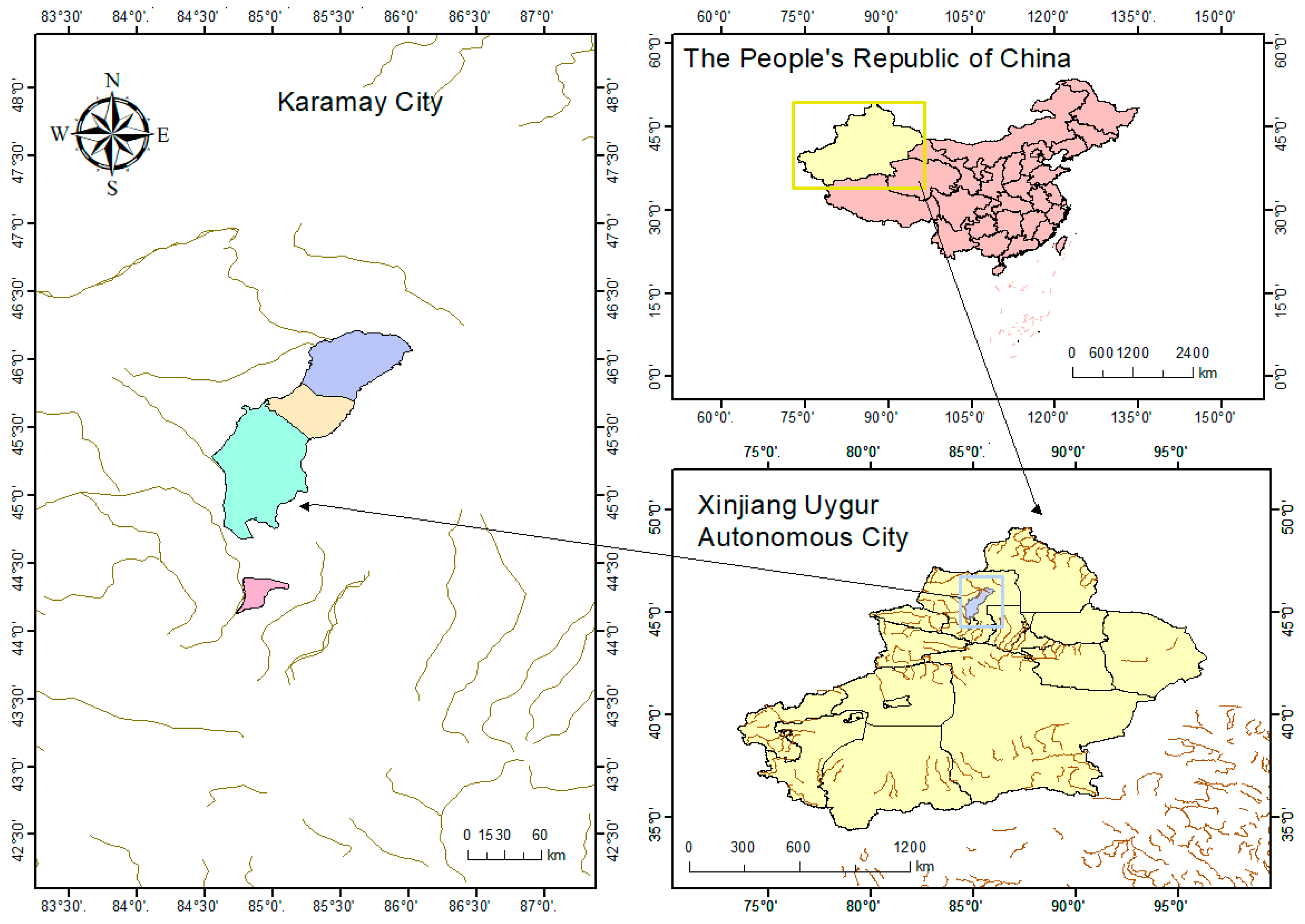
2.1. Overview of the Study Area
2.1.1. Study Area
2.1.2. Climate and River Characteristics
2.2. Data Collection
2.3. The Establishment of RFWQI Model
2.3.1. Indicator Selection
2.3.2. The Process of Determining Weight
Random Forest Model
Data Processing
Model Training
Hyperparameter Tuning
Random Forest Model Validation
2.3.3. Sub-Index Functions
2.3.4. Aggregation Function in WQI
2.3.5. Evaluation Disciplines
3. Results
3.1. Results of Indicator Selection
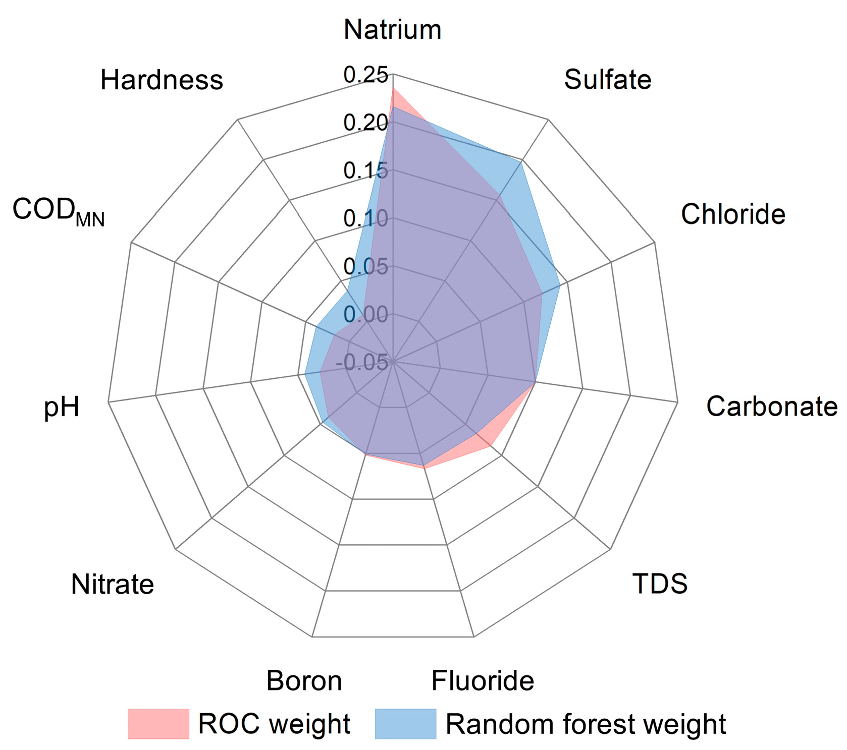
3.2. Weighting Calculation
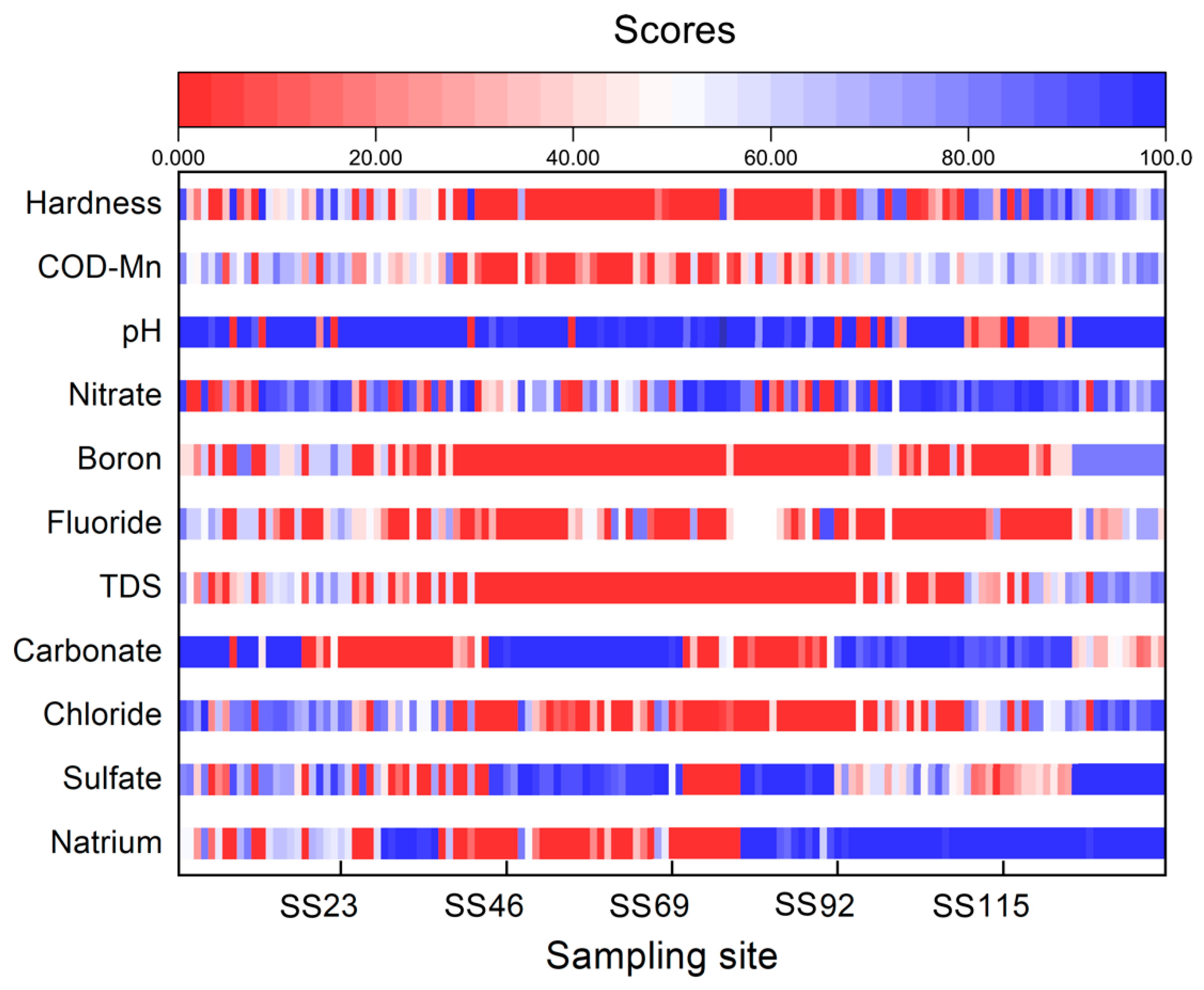
3.3. Indicator Scoring Results
3.4. Aggregate Function Calculation Results
3.5. Water Quality Evaluation Results
4. Discussion
4.1. Objective Selection of Indicators
4.2. Discussion of Weights Based on the Random Forest Model
4.2.1. Comparison of Different Weighting Methods
4.2.2. Hyperparameter Tuning for Random Forest Models
4.2.3. Random Forest Model Validation
4.3. The Effect of the Application of the Improved Sub-Indicator Function
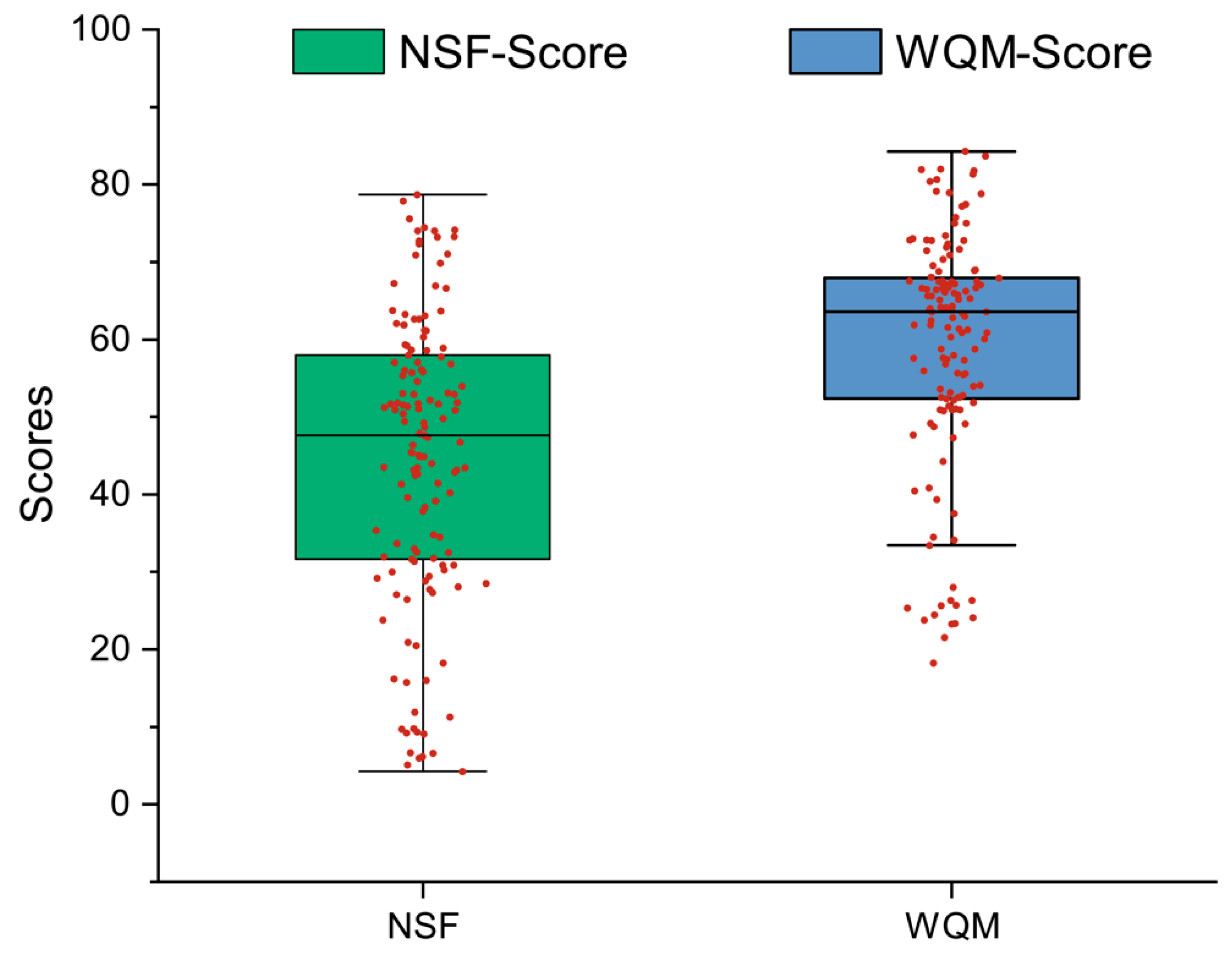
4.4. Comparison of Aggregation Effects of NSF and WQM
4.5. Comparison of Water Quality Evaluation Results
4.6. Comparison of Water Quality Evaluation Results
5. Conclusions
Supplementary Materials
Author Contributions
Funding
Institutional Review Board Statement
Informed Consent Statement
Data Availability Statement
Conflicts of Interest
References
- Li, N.; Lyu, H.; Xu, G.; Chi, G.; Su, X. Hydrogeochemical Changes during Artificial Groundwater Well Recharge. Sci. Total Environ. 2023, 900, 165778. [Google Scholar] [CrossRef]
- Uddin, M.G.; Nash, S.; Rahman, A.; Agnieszka, I. Olbert A Comprehensive Method for Improvement of Water Quality Index (WQI) Models for Coastal Water Quality Assessment. Water Res. 2022, 219, 118532. [Google Scholar] [CrossRef] [PubMed]
- Salehi, M. Global Water Shortage and Potable Water Safety; Today’s Concern and Tomorrow’s Crisis. Environ. Int. 2022, 158, 106936. [Google Scholar] [CrossRef] [PubMed]
- Jonsdottir, H.; Eliasson, J.; Madsen, H. Assessment of Serious Water Shortage in the Icelandic Water Resource System. Physics and Chemistry of the Earth, Parts A/B/C 2005, 30, 420–425. [Google Scholar] [CrossRef]
- Yang, P.; Zhang, S.; Xia, J.; Chen, Y.; Zhang, Y.; Cai, W.; Wang, W.; Wang, H.; Luo, X.; Chen, X. Risk Assessment of Water Resource Shortages in the Aksu River Basin of Northwest China under Climate Change. J. Environ. Manag. 2022, 305, 114394. [Google Scholar] [CrossRef] [PubMed]
- Zhao, K.; Fang, Z.; Li, J.; He, C. Spatial-Temporal Variations of Groundwater Storage in China: A Multiscale Analysis Based on GRACE Data. Resour. Conserv. Recycl. 2023, 197, 107088. [Google Scholar] [CrossRef]
- Sarami-Foroushani, T.; Balali, H.; Movahedi, R.; Kurban, A.; Värnik, R.; Stamenkovska, I.J.; Azadi, H. Importance of Good Groundwater Governance in Economic Development: The Case of Western Iran. Groundw. Sustain. Dev. 2023, 21, 100892. [Google Scholar] [CrossRef]
- Yang, T.; Zhu, Y.; Li, Y.; Zhou, B. Achieving Win-Win Policy Outcomes for Water Resource Management and Economic Development: The Experience of Chinese Cities. Sustain. Prod. Consum. 2021, 27, 873–888. [Google Scholar] [CrossRef]
- Wei, F.; Zhang, X.; Xu, J.; Bing, J.; Pan, G. Simulation of Water Resource Allocation for Sustainable Urban Development: An Integrated Optimization Approach. J. Clean. Prod. 2020, 273, 122537. [Google Scholar] [CrossRef]
- Zhao, E.; Kuo, Y.-M.; Chen, N. Assessment of Water Quality under Various Environmental Features Using a Site-Specific Weighting Water Quality Index. Sci. Total Environ. 2021, 783, 146868. [Google Scholar] [CrossRef]
- Akkoyunlu, A.; Akiner, M.E. Pollution Evaluation in Streams Using Water Quality Indices: A Case Study from Turkey’s Sapanca Lake Basin. Ecol. Indic. 2012, 18, 501–511. [Google Scholar] [CrossRef]
- Yang, X.; Chen, Z. A Hybrid Approach Based on Monte Carlo Simulation-VIKOR Method for Water Quality Assessment. Ecol. Indic. 2023, 150, 110202. [Google Scholar] [CrossRef]
- Barrie, A.; Agodzo, S.K.; Frazer-Williams, R.; Awuah, E.; Bessah, E. A Multivariate Statistical Approach and Water Quality Index for Water Quality Assessment for the Rokel River in Sierra Leone. Heliyon 2023, 9, e16196. [Google Scholar] [CrossRef] [PubMed]
- Benaissa, C.; Bouhmadi, B.; Rossi, A. An Assessment of the Physicochemical, Bacteriological Quality of Groundwater and the Water Quality Index (WQI) Used GIS in Ghis Nekor, Northern Morocco. Sci. Afr. 2023, 20, e01623. [Google Scholar] [CrossRef]
- Karangoda, R.C.; Nanayakkara, K.G.N. Use of the Water Quality Index and Multivariate Analysis to Assess Groundwater Quality for Drinking Purpose in Ratnapura District, Sri Lanka. Groundw. Sustain. Dev. 2023, 21, 100910. [Google Scholar] [CrossRef]
- Lee, H.; Park, S.; V-Minh Nguyen, H.; Shin, H.-S. Proposal for a New Customization Process for a Data-Based Water Quality Index Using a Random Forest Approach. Environ. Pollut. 2023, 323, 121222. [Google Scholar] [CrossRef] [PubMed]
- Mishra, M.; Singhal, A.; Srinivas, R. Effect of Urbanization on the Urban Lake Water Quality by Using Water Quality Index (WQI). Mater. Today Proc. 2023, in press. [Google Scholar] [CrossRef]
- Krishnamoorthy, N.; Thirumalai, R.; Lenin Sundar, M.; Anusuya, M.; Manoj Kumar, P.; Hemalatha, E.; Mohan Prasad, M.; Munjal, N. Assessment of Underground Water Quality and Water Quality Index across the Noyyal River Basin of Tirupur District in South India. Urban Clim. 2023, 49, 101436. [Google Scholar] [CrossRef]
- Uddin, M.G.; Nash, S.; Rahman, A.; Olbert, A.I. Performance Analysis of the Water Quality Index Model for Predicting Water State Using Machine Learning Techniques. Process Saf. Environ. Prot. 2023, 169, 808–828. [Google Scholar] [CrossRef]
- Uddin, M.G.; Nash, S.; Olbert, A.I. A Review of Water Quality Index Models and Their Use for Assessing Surface Water Quality. Ecol. Indic. 2021, 122, 107218. [Google Scholar] [CrossRef]
- Pesce, S.F.; Wunderlin, D.A. Use of Water Quality Indices to Verify the Impact of Córdoba City (Argentina) on Suquía River. Water Res. 2000, 34, 2915–2926. [Google Scholar] [CrossRef]
- Zhu, M.; Wang, J.; Yang, X.; Zhang, Y.; Zhang, L.; Ren, H.; Wu, B.; Ye, L. A Review of the Application of Machine Learning in Water Quality Evaluation. Eco-Environ. Health 2022, 1, 107–116. [Google Scholar] [CrossRef]
- Changfu, X.; Hongxian, L.; Genbao, Q.; Jianhua, Q. Microcosmic Mechanisms of Water-Oil Displacement in Conglomerate Reservoirs in Karamay Oilfield, NW China. Pet. Explor. Dev. 2011, 38, 725–732. [Google Scholar] [CrossRef]
- Cao, J.; Ma, S.; Yuan, W.; Wu, Z. Characteristics of Diurnal Variations of Warm-Season Precipitation over Xinjiang Province in China. Atmos. Ocean. Sci. Lett. 2022, 15, 100113. [Google Scholar] [CrossRef]
- Jha, M.K.; Shekhar, A.; Jenifer, M.A. Assessing Groundwater Quality for Drinking Water Supply Using Hybrid Fuzzy-GIS-Based Water Quality Index. Water Res. 2020, 179, 115867. [Google Scholar] [CrossRef] [PubMed]
- Prabagar, S.; Thuraisingam, S.; Prabagar, J. Sediment Analysis and Assessment of Water Quality in Spacial Variation Using Water Quality Index (NSFWQI) in Moragoda Canal in Galle, Sri Lanka. Waste Manag. Bull. 2023, 1, 15–20. [Google Scholar] [CrossRef]
- Wu, L.; Zhang, Y.; Wang, Z.; Geng, M.; Chen, Y.; Zhang, F. Method for Screening Water Physicochemical Parameters to Calculate Water Quality Index Based on These Parameters’ Correlation with Water Microbiota. Heliyon 2023, 9, e16697. [Google Scholar] [CrossRef]
- Karabadji, N.E.I.; Amara Korba, A.; Assi, A.; Seridi, H.; Aridhi, S.; Dhifli, W. Accuracy and Diversity-Aware Multi-Objective Approach for Random Forest Construction. Expert Syst. Appl. 2023, 225, 120138. [Google Scholar] [CrossRef]
- Hoarau, A.; Martin, A.; Dubois, J.-C.; Le Gall, Y. Evidential Random Forests. Expert Syst. Appl. 2023, 230, 120652. [Google Scholar] [CrossRef]
- Wang, S.; Qian, G.; Hopper, J. Integrated Logistic Ridge Regression and Random Forest for Phenotype-Genotype Association Analysis in Categorical Genomic Data Containing Non-Ignorable Missing Values. Appl. Math. Model. 2023, 123, 1–22. [Google Scholar] [CrossRef]
- Guo, W.; Gao, Z.; Guo, H.; Cao, W. Hydrogeochemical and Sediment Parameters Improve Predication Accuracy of Arsenic-Prone Groundwater in Random Forest Machine-Learning Models. Sci. Total Environ. 2023, 897, 165511. [Google Scholar] [CrossRef]
- GB/T14848-2017; Standard for Groundwater Quality. General Administration of Quality Supervision, Inspection and Quarantine of the PRC: Beijing, China, 2017.
- Ditton, E.; Swinbourne, A.; Myers, T. Selecting a Clustering Algorithm: A Semi-Automated Hyperparameter Tuning Framework for Effective Persona Development. Array 2022, 14, 100186. [Google Scholar] [CrossRef]
- Farhangi, F. Investigating the Role of Data Preprocessing, Hyperparameters Tuning, and Type of Machine Learning Algorithm in the Improvement of Drowsy EEG Signal Modeling. Intell. Syst. Appl. 2022, 15, 200100. [Google Scholar] [CrossRef]
- Gupta, S.C.; Goel, N. Predictive Modeling and Analytics for Diabetes Using Hyperparameter Tuned Machine Learning Techniques. Procedia Comput. Sci. 2023, 218, 1257–1269. [Google Scholar] [CrossRef]
- Kumar Ravi, N.; Kumar Jha, P.; Varma, K.; Tripathi, P.; Kumar Gautam, S.; Ram, K.; Kumar, M.; Tripathi, V. Application of Water Quality Index (WQI) and Statistical Techniques to Assess Water Quality for Drinking, Irrigation, and Industrial Purposes of the Ghaghara River, India. Total Environ. Res. Themes 2023, 6, 100049. [Google Scholar] [CrossRef]
- Ghosh, A.; Bera, B. Hydrogeochemical Assessment of Groundwater Quality for Drinking and Irrigation Applying Groundwater Quality Index (GWQI) and Irrigation Water Quality Index (IWQI). Groundw. Sustain. Dev. 2023, 22, 100958. [Google Scholar] [CrossRef]
- Rajkumar, H.; Naik, P.K.; Rishi, M.S. A Comprehensive Water Quality Index Based on Analytical Hierarchy Process. Ecol. Indic. 2022, 145, 109582. [Google Scholar] [CrossRef]
- Gupta, S.; Gupta, S.K. A Critical Review on Water Quality Index Tool: Genesis, Evolution and Future Directions. Ecol. Inform. 2021, 63, 101299. [Google Scholar] [CrossRef]
- Chandrajith, R.; Bandara, U.G.C.; Diyabalanage, S.; Senaratne, S.; Barth, J.A.C. Application of Water Quality Index as a Vulnerability Indicator to Determine Seawater Intrusion in Unconsolidated Sedimentary Aquifers in a Tropical Coastal Region of Sri Lanka. Groundw. Sustain. Dev. 2022, 19, 100831. [Google Scholar] [CrossRef]
- Haggerty, R.; Sun, J.; Yu, H.; Li, Y. Application of Machine Learning in Groundwater Quality Modeling—A Comprehensive Review. Water Res. 2023, 233, 119745. [Google Scholar] [CrossRef]
- Pan, B.; Han, X.; Chen, Y.; Wang, L.; Zheng, X. Determination of Key Parameters in Water Quality Monitoring of the Most Sediment-Laden Yellow River Based on Water Quality Index. Process Saf. Environ. Prot. 2022, 164, 249–259. [Google Scholar] [CrossRef]
- Jiang, M.; Wang, J.; Hu, L.; He, Z. Random Forest Clustering for Discrete Sequences. Pattern Recognit. Lett. 2023, 174, 145–151. [Google Scholar] [CrossRef]
- Josso, P.; Hall, A.; Williams, C.; Le Bas, T.; Lusty, P.; Murton, B. Application of Random-Forest Machine Learning Algorithm for Mineral Predictive Mapping of Fe-Mn Crusts in the World Ocean. Ore Geol. Rev. 2023, 162, 105671. [Google Scholar] [CrossRef]
- Sun, Z.; Wang, G.; Li, P.; Wang, H.; Zhang, M.; Liang, X. An Improved Random Forest Based on the Classification Accuracy and Correlation Measurement of Decision Trees. Expert Syst. Appl. 2024, 237, 121549. [Google Scholar] [CrossRef]
- Li, L.; Spratling, M. Understanding and Combating Robust Overfitting via Input Loss Landscape Analysis and Regularization. Pattern Recognit. 2023, 136, 109229. [Google Scholar] [CrossRef]
- Kim, J.; Park, H. Limited Discriminator GAN Using Explainable AI Model for Overfitting Problem. ICT Express 2023, 9, 241–246. [Google Scholar] [CrossRef]


| Indicator | Unit | WHO | Standard for Groundwater Quality |
|---|---|---|---|
| - | GB/T 14848-2017 [32] | ||
| pH | - | 6.5~8.5 | 6.5~8.5 |
| Total hardness 1 | mg/L | 500 | 450 |
| Sulfate | mg/L | 250 | 250 |
| Nitrate 2 | mg/L | 50 | 20 |
| Fluorine | mg/L | 1.5 | 1 |
| Natrium (Na) | mg/L | - | 200 |
| Chloride | mg/L | 250 | 250 |
| Carbonate | mg/L | - | 150 |
| Total dissolved solid | mg/L | 1000 | 1000 |
| Boron | mg/L | 0.3 | 0.5 |
| CODMN | mg/L | - | 3 |
| Confusion | Predicted Value | ||
|---|---|---|---|
| Negative | Positive | ||
| True Value | Negative | True Negative | False Positive |
| Positive | False Negative | True Positive | |
| Aggregate Function Name | Calculation Formula |
|---|---|
| NSF index (Weighted Arithmetic Mean) | |
| Weighted Quadratic Mean (WQM) |
| WQI Models | Evaluation Catagories |
|---|---|
| NSF index | (1) excellent (90~100) (2) good (70~89) (3) medium (50~69) (4) bad (25~49) (5) very bad (0~24) |
| CCME | (1) excellent (95~100) (2) good (80~94) (3) medium (65~79) (4) bad (45~65) (5) very bad (0~44) |
| Hanh Index | (1) excellent (91~100) (2) good (76~90) (3) medium (51~75) (4) bad (26~50) (5) very bad (<25) |
| RFWQI | (1) excellent (92~100) (2) good (70~91) (3) medium (51~69) (4) poor (26~50) (5) unacceptable (0~25) |
| Hyperparameter | Default Results | Tuning Results |
|---|---|---|
| N_estimators | Default value | 120 |
| Max_depth | Default value | 4 |
| Min_sample_split | Default value | 2.1 |
| Min_sample_leaf | Default value | 1.05 |
| Accuracy | 0.86 | 0.96 |
| RMSE | 0.377 | 0.188 |
| Iteration | Evaluating Indicator | |||
|---|---|---|---|---|
| Accuracy | AUC | RMSE | F1-Score | |
| 1 | 0.893 | 0.75 | 0.327 | 0.936 |
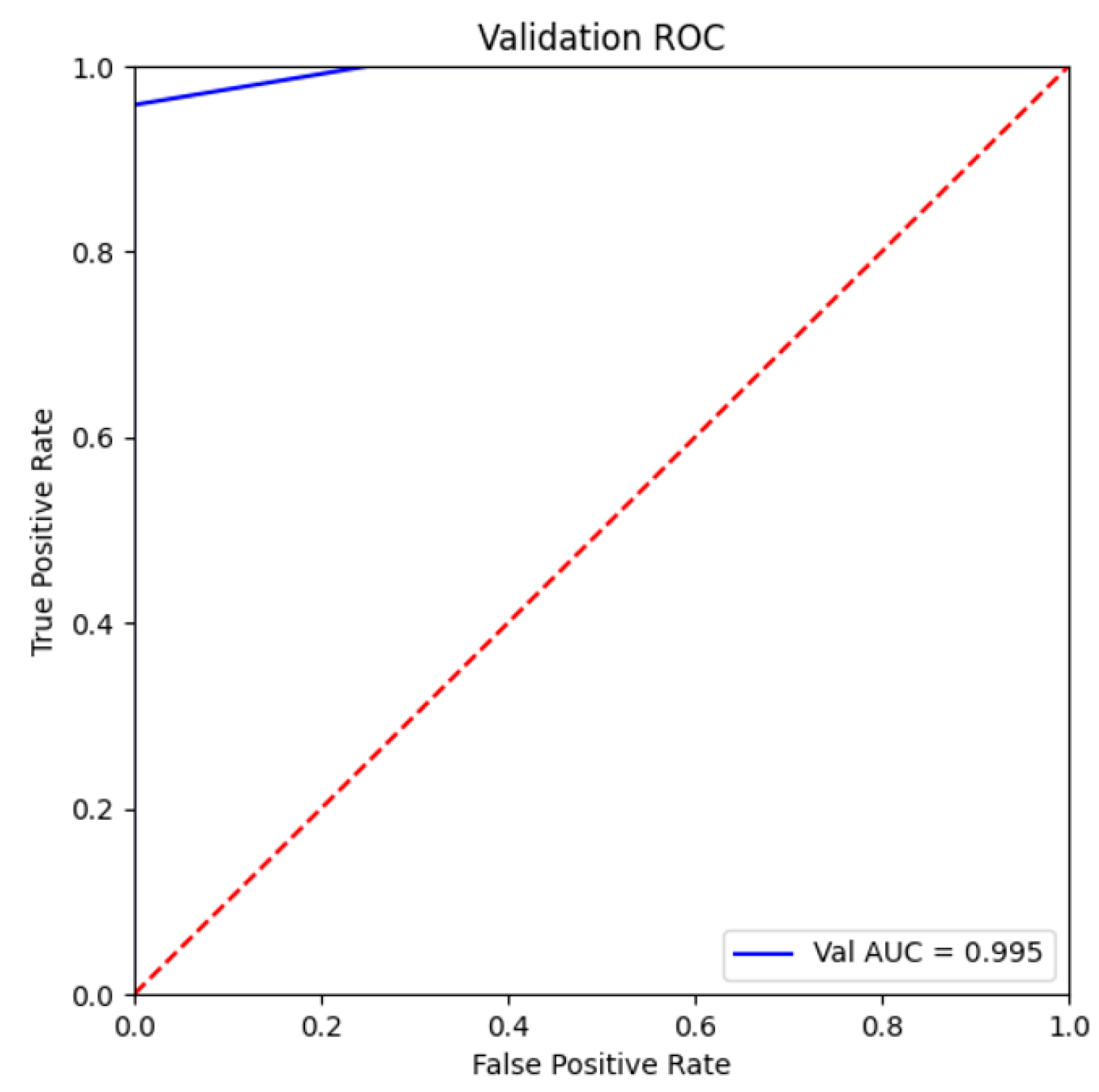
| 2 | 0.964 | 0.995 | 0.189 | 0.98 |
| 3 | 0.964 | 0.995 | 0.189 | 0.98 |
| 4 | 0.928 | 0.8 | 0.267 | 0.958 |
| 5 | 0.964 | 0.995 | 0.189 | 0.98 |
| Mean value | 0.94 | 0.91 | 0.232 | 0.967 |
| Aggregation Functions | Groundwater Quality Classifications | |||||||
|---|---|---|---|---|---|---|---|---|
| NSF | Good (8) * | Medium (49) | Poor (54) | Unacceptable (20) | ||||
| U | O | U | O | U | O | U | O | |
| 0 (0%) | 0 (0%) | 8 (16.3%) | 0 (0%) | 10 (18.5%) | 0 (0%) | 4 (20%) | 0 (0%) | |
| WQM | Good (8) | Fair (103) | Marginal (13) | Poor (13) | ||||
| U ** | O | U | O | U | O | U | O | |
| 0 (0%) | 0 (0%) | 16 (15.5%) | 43 (41.7%) | 4 (30.7%) | 6 (46.1%) | 2 (15.4%) | 0 (0%) | |
Disclaimer/Publisher’s Note: The statements, opinions and data contained in all publications are solely those of the individual author(s) and contributor(s) and not of MDPI and/or the editor(s). MDPI and/or the editor(s) disclaim responsibility for any injury to people or property resulting from any ideas, methods, instructions or products referred to in the content. |
© 2023 by the authors. Licensee MDPI, Basel, Switzerland. This article is an open access article distributed under the terms and conditions of the Creative Commons Attribution (CC BY) license (https://creativecommons.org/licenses/by/4.0/).
Share and Cite
Xiong, Y.; Zhang, T.; Sun, X.; Yuan, W.; Gao, M.; Wu, J.; Han, Z. Groundwater Quality Assessment Based on the Random Forest Water Quality Index—Taking Karamay City as an Example. Sustainability 2023, 15, 14477. https://doi.org/10.3390/su151914477
Xiong Y, Zhang T, Sun X, Yuan W, Gao M, Wu J, Han Z. Groundwater Quality Assessment Based on the Random Forest Water Quality Index—Taking Karamay City as an Example. Sustainability. 2023; 15(19):14477. https://doi.org/10.3390/su151914477
Chicago/Turabian StyleXiong, Yanna, Tianyi Zhang, Xi Sun, Wenchao Yuan, Mingjun Gao, Jin Wu, and Zhijun Han. 2023. "Groundwater Quality Assessment Based on the Random Forest Water Quality Index—Taking Karamay City as an Example" Sustainability 15, no. 19: 14477. https://doi.org/10.3390/su151914477
APA StyleXiong, Y., Zhang, T., Sun, X., Yuan, W., Gao, M., Wu, J., & Han, Z. (2023). Groundwater Quality Assessment Based on the Random Forest Water Quality Index—Taking Karamay City as an Example. Sustainability, 15(19), 14477. https://doi.org/10.3390/su151914477