Modeling the Hydraulic Performance of Pilot Green Roofs Using the Storm Water Management Model: How Important Is Calibration?

Abstract

Green roofs are low-impact development (LID) that assist in regulating stormwater runoff by reducing the peak flow rate and total runoff volume, among other benefits. In this study, the hydraulic performance of green roofs was modeled using the SWMM 5.2 software, taking field data into account for calibration purposes. A Storm Water Management Model (SWMM) was built using field data from pilot green roofs installed at the Instituto Superior Técnico Campus, University of Lisbon, Portugal. The simulated results with and without calibration were compared, as well as the results obtained in the field studies. The results from the uncalibrated model were unsatisfactory. After calibration, the average Nash–Sutcliffe model efficiency (NSE) was 0.72, and the volume error was 5.9%, with most of the results classified as very good and good. This study shows relevant insights on the use of the SWMM to model green roofs, demonstrating the crucial importance of the calibration process for the correct prediction of hydraulic performance and indicating the porosity parameter as one of the most sensitive to the results. In addition, it provides estimates of LID parameters that can help in the development of projects carried out in the Mediterranean climate.

1. Introduction

1.1. Background

In a context of growing urbanization and increasing impervious areas, stormwater management represents a major challenge for cities [1]. The implementation of urban green infrastructure, in parallel with existing gray infrastructure, is a way to benefit urban areas, namely with the reduction in urban surface runoff. These green solutions, also called low-impact development (LID), are source control measures, which are considered an effective strategy in stormwater management [2,3].

Green roofs are one of the LID measures, and they have become increasingly popular as they assist in regulating stormwater runoff by reducing the peak flow rate and total runoff volume [4,5,6,7].

In order to effectively design and manage green roofs for stormwater management purposes, it is important to understand how different factors influence their hydrological performance. Several studies have focused on understanding the impact of different factors on green roof performance, such as substrate characteristics and composition [8,9,10]; roof geometry [4,11]; and natural factors, such as weather conditions and precipitation patterns [12,13]. The large number of factors affecting the performance of green roofs explains the high variability of retention results that are reported in studies [14]. Retention is defined by the difference between the total depth of precipitation and the total depth of runoff, divided by the total depth of precipitation [1]. When comparing the results of three different studies on green roofs, the retention performances ranged between 10% and 91% for rainfall depths ranging from 0.13 to 41.6 mm [1,15,16]. This variability found in research makes it difficult to estimate the retention performance of green roofs, even when field data are present [14,17].

Thus, even though the positive effects of green roofs are proven, it can be challenging to estimate their precise quantitative impact as the performance per green roof per rainfall event varies greatly [18]. A possible estimation approach could be using a hydraulic–hydrologic model that simulates the green roof and its runoff, peak flow, and retention volume. This would also allow green roofs to be modeled as part of a local city’s comprehensive stormwater management plan [19]. Having a more accurate prediction on the green roof performance would contribute to decision making regarding NBS investments in urban areas.

There are a number of studies available about the Storm Water Management Model (SWMM), a software commonly used for hydraulic–hydrological models, applied on green roofs. However, the retention results considerably vary. The performance of the model is strongly conditioned by its location, due to the impact of layer materials, vegetation, physical substrate properties, design specifications, and climatic conditions [15,20,21,22]. Therefore, as pointed out by Iffland et al. [22] and Cipolla [15], field research analyzing hydraulic modeling should be carried out in different climate zones to investigate the effect of climate on parameter optimization. The type of model chosen varies within the literature as well. Within the SWMM, there are two options to model a green roof: using the bioretention cell LID control or green roof LID control [20]. Some studies discuss the use of bioretention cells [15,20,23,24], whereas others consider green roof function [14,22,25,26,27]. Jeffers et al. [19] used both. Among the same LID controls, sometimes different conclusions are reached. An example is Burszta and Mrowiec [20] and Cipolla [15], who reached divergent conclusions despite having used the bioretention cell LID control.

Although there are several studies regarding green roofs in Mediterranean climates [1,28,29,30,31,32,33,34,35,36,37,38], only a small number of articles involve modeling analyses, such as the studies by Palla et al. [35] and Barnhart et al. [38], and even fewer have used the SWMM [30,34,39]. Thus, there are only a few studies that have validated the capability of models that represent the hydrological performance of extensive green roofs in response to extreme or frequent rainfall events in Mediterranean climates.

Mediterranean climates have particular characteristics. Normally, they have very dry summers with short, intense rainfall periods concentrated in the winter [1,16,28,39].

This paper aims to fill the knowledge gap in modeling the hydrological performance of green roofs in Mediterranean climates. Therefore, the goal is to evaluate the accuracy of the latest version of the SWMM (SWMM 5.2) and demonstrate the importance of the calibration process to model the hydraulic performance of green roofs with the SWMM software, providing practical insights into the use of this LID technique in projects located in Mediterranean climates. To achieve these objectives, field data from extensive pilot green roofs located in the city of Lisbon, Portugal, were used for model calibration and validation. A comparison between the modeled and field-measured runoff was performed. An additional comparison was made between the calibrated model and a second, uncalibrated model that uses the default SWMM values to quantify the impact of calibration on model performance.

1.2. Hydraulic–Hydrologic Modeling: SWMM

There are many different software that support green roof modeling. In this paper, the Storm Water Management Model (SWMM) software was used. The SWMM software is developed by the United States Environmental Protection Agency and is used worldwide by both academics and regulatory bodies [19].

The SWMM is an open source dynamic rainfall–runoff simulation model used to predict contributing sub-basin flows and analyze wastewater and stormwater flow in piped systems [40].

The first version of the SWMM was released in 1971, and it has been continually updated ever since [26]. In 2010, an LID module was implemented that allows for the simulation of bioretention cells, permeable sidewalks, and infiltration [41]. In 2014, the SWMM green roof LID module was first introduced [14].

The SWMM green roof LID is composed of three layers, namely the surface layer, the soil layer, and the drainage layer, which represent the typical green roof layers [40]. Each layer is defined by a set of parameters that influence the hydraulic behavior of green roofs.

The conceptual model of LID controls is shown in Figure 1. In the left model, the top left arrow represents the inflow, in the present case, the artificial rainfall, which is evenly distributed over the soil. The top right arrow shows the surface runoff. This was not considered in the present case, as low-intensity rainfalls were simulated, and the berm height was 100 mm. The bottom blue arrow represents the drainage outflow. As is shown in the right model, runoff flows over the entire width of the sub-catchment.

In the green roof LID control, the drainage of the green roof is governed by Manning’s equation (Equation (1)) [40].

$$Q_3=\frac{1}{n}\sqrt{S}\left(\frac{W}{A_{LID}}\right){\varphi }_3{\left(d_3\right)}^{\frac{5}{3}},$$

(1)

where $Q_3$ is the drainage layer outflow, n is the drainage layer roughness, S is the slope of the green roof, W is the total length along the edge of the roof where runoff is collected, $A_{LID}$ is the area of the LID control, $d_3$ is the hydraulic head in the drainage layer, and ${\varphi }_3$ is the drainage layer void fraction.

Since monitoring large-scale green roof installations presents several obstacles for high-accuracy measurements, such as unpredictable weather and antecedent moisture conditions, this study used small-scale green roofs, where the environment could be more controlled, which gives the opportunity to quickly test and measure several different rainfall patterns and antecedent moisture initial conditions [19].

The model was built considering the physical dimensions and properties of the pilot green roofs located at the Instituto Superior Técnico (IST) Campus, University of Lisbon, Portugal. Unknown parameters were mainly based on findings in the literature.

1.3. Sensitivity Analysis

The unknown parameters were explored through sensitivity analysis and calibration. A sensitivity analysis of the SWMM parameters helps to understand the parameters and their effect on the model outputs, namely the total runoff volume and peak flow. In this section, five different sensitivity analyses are examined, all executed by different authors [19,24,25,26,27]. These outcomes are used to calibrate the model since they show which parameters should be prioritized and ignored during the calibration process.

Limos et al. [24] and Peng and Stovin [25] calculated parameter sensitivity with Equation (2) [42]. In this equation, the condition number (CN) is calculated. Larger values of CN mean a higher sensitivity of the parameter

$$\mathrm{CN}=\frac{k∆c}{c∆k}$$

(2)

In Equation (2), k is the base parameter value, c is the corresponding base runoff, $∆k$ is the change in parameter, and $∆c$ is the change in runoff prediction. A positive value implies that there is a direct relationship between the parameter and the output, whereas a negative CN implies that there is an inverse relationship.

Krebs et al. [26] calculated the parameter sensitivity using the generalized likelihood uncertainty estimation (GLUE) procedure. They ran the model over 50,000 times. All parameters were analyzed, except for the three physical parameters berm height, slope, and soil thickness. Jeffers et al. [19] performed a sensitivity analysis on both the Green Roof and the bioretention cell LID control using the sensitivity-based radio tuning calibration (SRTC) tool in Personal Computer SWMM, varying parameters one by one between a range of 50% and 200%. Paithankar and Taji [27] repeated simulations each time, adjusting a single parameter at a time and observing its effect on the model outputs. During this process, Paithankar and Taji [27] changed the values of the parameter over a range of ±30% of their original value. The findings of all five studies are summarized in

Table 1. SWMM parameters for green roofs (adapted from [43]).

Parameter	Limos et al. [24]		Peng and Stovin [25]		Krebs et al. [26]	Jeffers, Garner et al. [19]		Leimgruber et al. [44]
	RV	PF	RV	PF	RV&PF	RV	PF	RV	PF
Porosity	NS	-	S	S	S	S	S	S	-
Soil thickness	NS	-	-	-	-	S	S	S	-
Surface roughness	NS	-	NS	NS	NS	NS	NS	NS	-
Void fraction	NS	-	NS	NS	S	NS	S	NS	-
Surface slope	NS	-	NS	NS	-	NS	S	NS	-
Conductivity slope	NS	-	S	S	S	S	S	-	-
Hydraulic width	NS	-	-	-	-	NS	S	-	-
Vegetation cover	NS	-	-	-	NS	S	S	NS	-
Wilting point	S	-	S	S	S	S	NS	-	-
Soil conductivity	NS	-	-	-	S	NS	NS	-	-
Surface roughness	NS	-	-	-	-	NS	NS	-	-
Field capacity	S	-	S	S	S	S	NS	S	-
Suction head	NS	-	NS	NS	NS	NS	NS	NS	-
Thickness (mat)	NS	-	-	-	-	NS	NS	NS	-
Berm height	NS	-	-	-	-	NS	NS	NS	-
Roughness (mat)	NS	-	-	-	S	NS	S	NS	-
Evaporation rate	S	-	S	S	S	-	-	-	-

RV—runoff volume, PF—peak flow, NS—not sensitive, S—sensitive.

.

Table 1 shows sensitivity analysis results for the parameters’ porosity, soil thickness, conductivity slope, wilting point, field capacity, and evaporation rate. The latter was not considered in the present study as evaporation was not measured. Limos et al. [24] and Leimgruber et al. [44] only focused on the total runoff volumes and did not run a sensitivity analysis considering peak flows. From the other studies, however, it can be concluded that 10 out of 16 times, the sensitivity analysis using peak flows tends to have approximately the same results as the sensitivity analysis using runoff volumes. Exceptions are on the parameters’ void fraction, surface slope, hydraulic width, wilting point, field capacity, and roughness of the drainage mat.

2. Materials and Methods

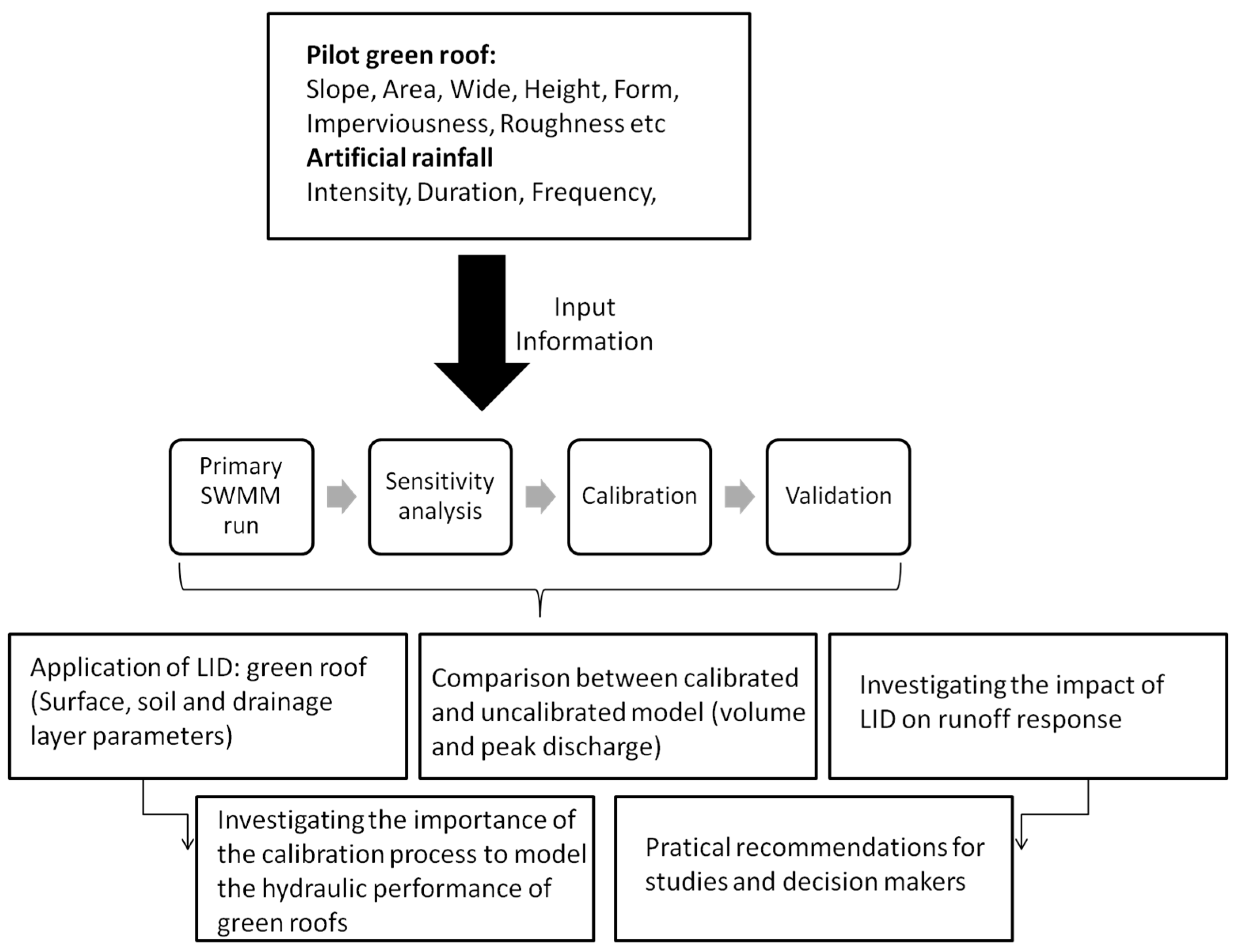
2.1. Research Steps

The process of this research followed the steps shown in Figure 2. In the first step, the input data for the SWMM were collected through field measurements, using artificial rainfall on a pilot green roof. In the subsequent step, these data were used to build a draft model in the SWMM. The calibration and validation processes were supported by previously mentioned sensitivity analyses.

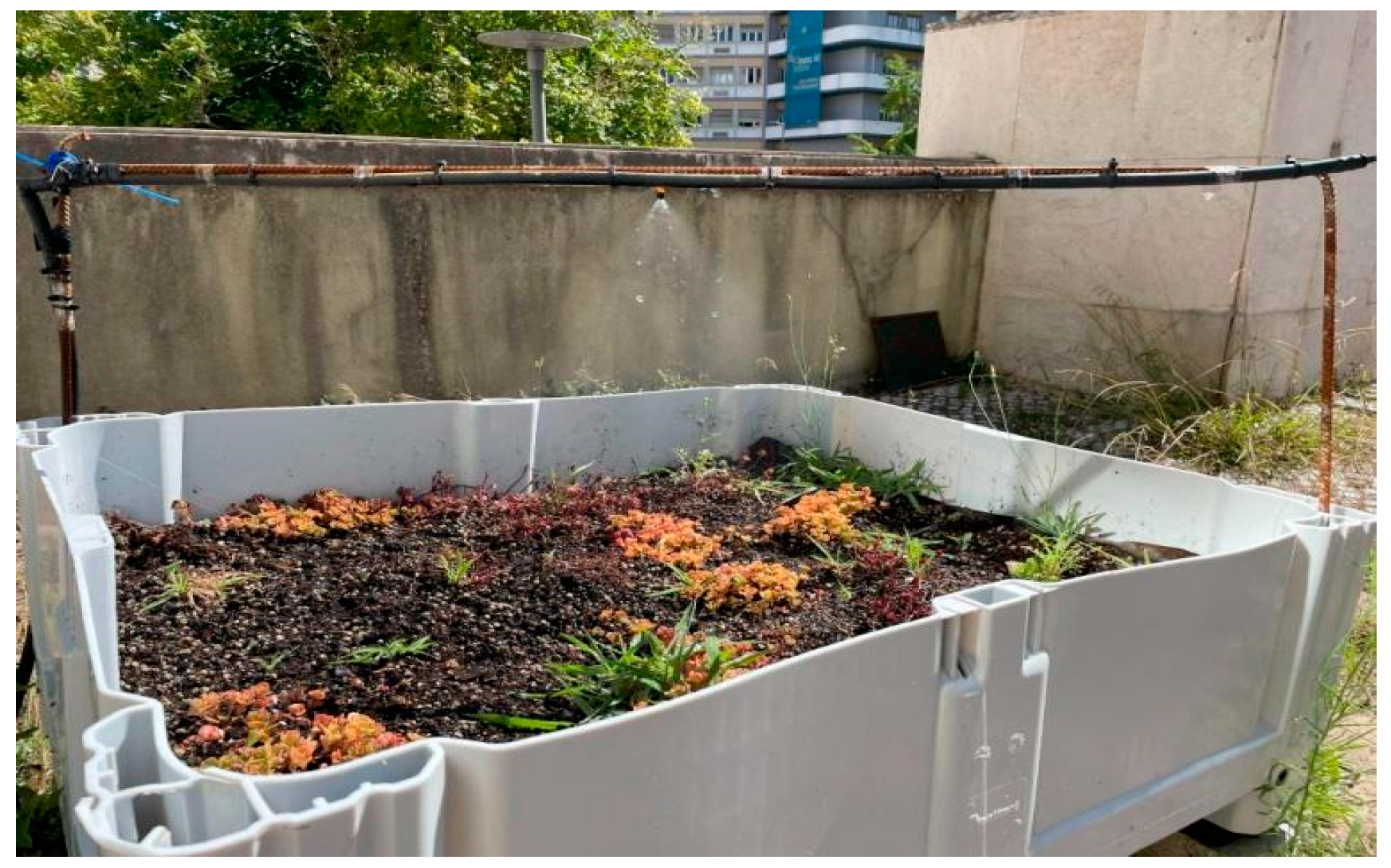
2.2. Pilot Green Roofs

The field data were collected from an extensive pilot green roof, located at the Instituto Superior Técnico (IST) Campus. The test beds were built in December 2020, as described in a study by Santos et al. [16], using a 676 L HDPE pallet box with external dimensions of 1.20 × 1.00 × 0.78 m (internal dimensions are 1.12 × 0.92 × 0.61 m), 10 cm depth, and 2° slope, and included a discharge channel at the lowest point of the green roof for the runoff to exit, against the side wall. The structure of the green roof is multilayered. It consists of vegetation, substrate, filtering layer, drainage layer, and protective blanket. The drainage layer was composed of modular drainage panels from Floradrain FD25, ZinCo International (Hereford, UK). These panels, made from recycled polyolefin material, have a thickness of 25 mm [45]. The material of the box is waterproof, fulfilling the function of the waterproofing membrane, which is a layer commonly present in the structure of green roofs. The substrate consists of 21% organic matter with vegetation of mixed species (Sedum album, Sedum sexangular, Sedum spurium, Sedum spurium tricolor, Sedum coral reef, Sedum oreganum, and Sedum forsteriamum) that are well adapted to the Mediterranean climate. An overview of the substrate characteristics is shown in

Table 2. Substrate characteristics of the green roof test beds.

Parameters	Substrate
pH (H2O)	7.1
Nitric nitrogen (mg/L)	3.3
Extractable phosphorus (mg/L)	<1.0
Extractable potassium (mg/L)	35.9
Organic matter (%)	20.9
Dry matter (%)	54.4
Density (g/cm3)	0.53
Fine fraction (%)	26.2
Coarse fraction (%)	73.8
Sand fraction (%)	45.1
Slime fraction (%)	34.3
Clay fraction (%)	20.6

.

Lisbon is located in a typical Mediterranean climate zone, which is characterized by dry and hot summers and wet winters [46]. The long-term (1960–2022) average total precipitation in Lisbon is 766.9 mm [47], but precipitation is concentrated mainly in winter, between the months of October and April [46]. In 2022, for example, 70% of the year’s precipitation occurred in the last four months of the year [46]. The average number of days without rain, considering the period from 1960 to 2022, was approximately 255 days, and the average annual temperature for the same period was 17.2 °C [47].

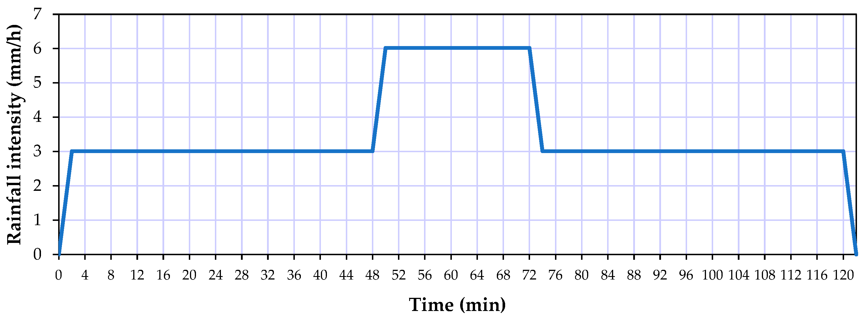
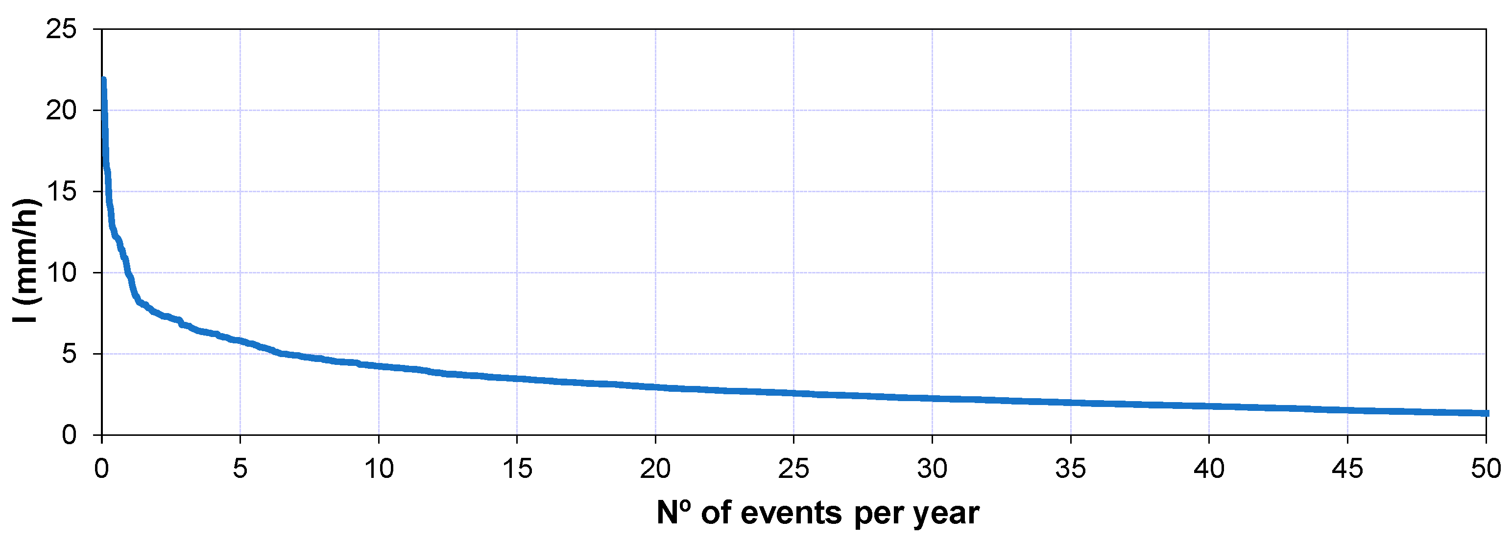
2.3. Data Collection

For this research, two experimental campaigns were carried out. The first campaign occurred between April and August 2022 and the second in April 2023.

In the first campaign, artificial rainfalls were of medium and high intensity, between 40 and 92 mm/hour, with constant durations of 20 min (simulating strong storms according to the Portuguese Institute of Sea and Atmosphere (IPMA)). Constant rainfall intensities were considered, as usually applied for the design of hydraulic urban infrastructures in small catchments, according to the national legislation (Regulatory Decree No 23/95 of 23 August). Consequently, a constant intensity for these short rainfall durations was maintained. The second campaign consisted of 2 h artificial rainfalls that varied in intensity over time. This rainfall distribution pattern is shown in Figure 3. As depicted in the graph, the rainfall pattern can be divided into three different blocks: two 48 min blocks with a 24 min peak in between. The middle block has twice the intensity of the first and third blocks. For this second campaign, low rainfall intensities were used, with an average of 3.46 mm/h. The experiments approximately simulated typical critical rainfall events of Lisbon’s small catchments: rainfall events with a frequency of about fifteen times a year. The characteristics of these rainfall events were set based on data from intensity–duration–frequency (IDF) curves (Figure 4) for relatively low-intensity rainfalls [48].

Rainfall was simulated using a garden irrigation sprayer mounted on a hose, which was attached to a cast iron frame placed above the test bed (Figure 5). Water supply from the public water network was used. Before each experiment, the system’s flow was measured so that the selected artificial rainfall intensity was ensured. The runoff was collected and weighed in five-minute intervals. The measured runoff of all events can be found in the Supplementary Materials of this paper in Tables S1–S15. Because the pilot beds were small (1.03 m²), the homogenous distribution of the artificial rainfall could be controlled. Furthermore, throughout all experiments, people were present to oversee and supervise the rainfall distribution and runoff collection. For this second campaign, low intensities were used, with an average of 3.46 mm/h. The experiments simulated typical rainfall events of Lisbon: rainfall events with a frequency of fifteen times a year. The characteristics of these rainfall events were set based on data from intensity–duration–frequency (IDF) curves (Figure 4) for relatively low-intensity rainfalls [49].

To ensure wet conditions and replicate the impact of rainfall events after wet periods (the ones with more impact in terms of flooding risks), the substrates were saturated twelve hours before testing. This was carried out by ponding the pilot bed before letting the water drain out.

The soil humidity of the pilot green roofs was measured 24 h before, at time zero, immediately after a rainfall event, 24 h after, 3 days after, and 7 days after the experiment to obtain accurate estimates of the soil conditions. A humidity sensing probe (Campbell Scientific (North Logan, UT, USA)—HydroSence II) was used. The measurements were taken at five surface points, and then the measurements were averaged.

In the SWMM, soil moisture should be set to the same condition as measured in pilot beds before executing experiments. However, as Jeffers et al. [19] pointed out, the SWMM has a limitation regarding the initial soil moisture conditions. If one tries to set the initial soil moisture of the green roof soil, the moisture content of the drainage layer is affected as well. As a result, in the simulation the runoff occurs immediately, which does not happen in reality. A way to bypass this problem is adding an extra rainfall event, which will saturate the soil. This approach is also used in the research of Jeffers et al. [19]. The volume of pre-rainfall was dependent on the measured humidity of the test beds prior to each experiment.

Measuring the performance of green roofs during critical soil moisture conditions is important because flood events normally occur after preceding days of rain.

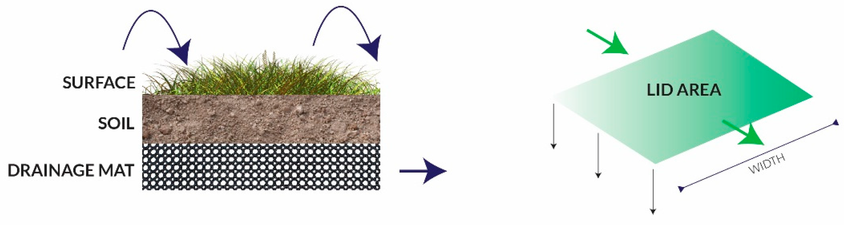
2.4. Applying SWMM 5.2

2.4.1. Fixed Model Settings

In the SWMM, a green roof was modeled by placing a green roof LID control on top of an entire sub-catchment. The area of the LID control therefore corresponded to the area of the sub-catchment. The model parameters were based on the physical properties of the pilot green roof, with values taken from the literature and through the calibration of the model. An overview of all the fixed parameters is shown in

Table 3. Fixed SWMM parameters: values and units.

Parameter	Value	Unit	Obtained through:
Area sub-catchment	0.000103	ha	Field measurement
Slope	2	%	Field measurement
Berm height	110	mm	Field measurement
Vegetation volume fraction	0.1	m3/m3	SWMM Reference Manual
Surface roughness (Manning’s n)	0.1	-	SWMM Reference Manual
Soil thickness	101	mm	Field measurement
Porosity	0.457	m3/m3	Field measurement
Conductivity	5555	mm/h	Field measurement
Suction head	88.9	mm	SWMM Reference Manual
Drainage mat thickness	25	mm	Field measurement
Void fraction	0.5	m3/m3	Field measurement
Hydraulic width	1	m	Field measurement

. General settings are also worth noting. Flow units were set to cubic meters per second (CMS), so SI units were used throughout. The infiltration model was set to the modified Green–Ampt method. The flow routing was the dynamic wave.

2.4.2. Model Calibration and Validation

The parameters conductivity slope, wilting point, and field capacity showed a significant sensitivity and were selected for calibration. Other parameters that showed a particular sensitivity were soil thickness, hydraulic width, and porosity. However, these parameters could be physically measured and therefore did not require calibration. Parameters that were not found to be sensitive and that could not be measured using the physical pilot beds were based on the literature.

The SWMM was manually calibrated using data from twelve experiments of different rainfall intensities. The objective functions for calibration were the Nash–Sutcliffe efficiency (NSE) coefficient and the volume error (VE). The NSE coefficient is a statistical measure commonly used in hydrological or hydrodynamic models. It compares the observed values to the predicted and quantifies the model’s ability to reproduce the observed data. The NSE coefficient ranges from negative infinity to 1, with 1 indicating a perfect prediction of the model. Modeling NSE results for different rainfall events can be analyzed using the following scale, also used by other authors [19,50]: Very good, >0.75; Good, 0.65–0.75; Satisfactory, 0.5–0.65; and Unsatisfactory, <0.5. The coefficient is calculated with Equation (3), where $\underset{\_}{Q_o}$ represents the observed runoff, and $Q_{m, i }$ is the modeled runoff [51].

$$\mathrm{NSE}=\frac{{\sum }_{i=1}^n{\left(Q_{o, i }- Q_{m, i}\right)}^2}{{\sum }_{i=1}^n{{(Q}_{o, i }- \underset{\_}{Q_o})}^2}$$

(3)

The VE is another statistical measure used to assess the accuracy of hydrological or hydrodynamic models. It quantifies the difference between the predicted and observed volumes of runoff water over a specified period. A lower volume error indicates better model performance, with values close to 0 indicating a good match between the model’s predicted volume and the observed volume. Acceptable values are in the range between −20% and 20%. The VE is calculated with Equation (4) [14,51], where $V_{o }$ is the observed volume runoff, and $V_m$ is the modeled volume runoff.

$$\mathrm{VE}=\frac{V_{o }-V_m}{V_{o }}\times 100$$

(4)

To validate the model, it was tested on seven different rainfall experiments: three with two hours of duration and low-intensity rainfall (more frequent rainfalls in Lisbon) and the others with twenty minutes of duration with higher rainfall intensities. The model was run with the same parameter settings, only changing the time series. The NSE coefficient and the VE were again used to evaluate the model.

2.4.3. Comparing Calibrated and Uncalibrated Simulation Approaches

To evaluate the accuracy of the SWMM, and to demonstrate and quantify the importance of the calibration process, two different green roof LID controls were compared:

• One calibrated LID control based on the geometric and physical measured characteristics of the test beds, including the measured hydraulic conductivity and porosity;
• One uncalibrated LID control based on the geometric and physical measured characteristics but with the remaining parameters, including the hydraulic conductivity and porosity, set to the default settings of SWMM 5.2.

The objective of using these approaches was to compare the results provided by each model with the results observed in the pilot green roofs, determining the NSE and the VE for both scenarios. We also aimed to evaluate to what extent the use of a calibrated model, with all the work that it requires, is justified and translates into a significant improvement of the results obtained by modeling when compared to the use of an uncalibrated model. This is useful, especially for field practitioners who often face limitations when calibrating and validating models.

3. Results and Discussion

3.1. Calibration and Validation Results

Ten experiments of 20 min duration with medium and high rainfall intensities (ranging from 45 to 92 mm/h) were selected for the calibration process, and five experiments with low and medium intensities (ranging from 3.5 to 56 mm/h) were selected for validation purposes. The final parameter values found in the calibration process, as well as its lower and upper limits (minimum and maximum) [26], are shown in

Table 4. Calibrated parameters.

Parameter	Value	Unit	Min–Max
Field capacity	0.31	m3/m3	0.11–0.34
Wilting point	0.004	m3/m3	0–0.1
Conductivity slope	53	-	0.1–40
Roughness (Manning’s number)	0.4	-	0.001–2

. In

Table 5. NSE and volume error results for calibration and validation.

Date	Average Rainfall Intensity (mm/h)	Rainfall Duration (Minutes)	Test Type	NSE	VE (%)
03-05-22	92.0	20	Calibration	0.98	2.98
27-04-22	55.2	20	Calibration	0.64	17.87
13-04-22	71.3	20	Calibration	0.70	10.71
12-04-22	44.8	20	Calibration	0.61	0.88
14-04-22	92.0	20	Calibration	0.58	6.19
05-05-22	55.2	20	Calibration	0.66	3.00
18-08-22	73.8	20	Calibration	0.72	6.45
19-08-22	92.0	20	Calibration	0.74	7.16
22-08-22	92.0	20	Calibration	0.83	2.49
24-08-22	77.1	20	Calibration	0.76	1.68
25-08-22	40.0	20	Validation	0.59	4.55
30-08-22	55.8	20	Validation	0.69	0.18
18-04-23	3.5	120	Validation	0.91	−5.50
21-04-23	3.5	120	Validation	0.89	1.00
25-04-23	3.5	120	Validation	0.72	−4.24

, the NSE and volume errors for calibration and validation are presented.

Around 73% of the events were rated very good and good according to the previously mentioned scale. The average NSE value for calibration was approximately 0.72, and the volume error was around 5.9%, which is considered very good. For validation, the average NSE increased to 0.76, and the VE reached approximately 3.1%. When considering all events together, the average values were around 0.73 and 5% for NSE and VE, respectively.

According to this scale, the results of the calibration and validation process were successful for rainfall events of different durations and intensities. An interesting aspect of this research is that this calibrated model was also validated (e.g., complying with the error criteria) when simulating the low-intensity rainfalls (out of the calibration rainfall intensity data range). Varying results have been presented in the literature for similar approaches. Some authors found good values for both calibration and validation, having most NSE scores above 0.5 [14,52,53]. Not only their NSE scores but also their VE show promising results, with ranges between 3% and 29% [51]. On the other hand, there are also studies that reach the opposite conclusion, showing that, even with good values for calibration, for validation, the model still has NSE scores lower than 0.5 [19,20,26]. It should be noted that negative values were also obtained with calibration.

To calibrate the model in this study, high-intensity rainfall events were used, and then validation was performed for less intense events. The result of this validation showed a good fit for the less intense events (events on 18, 21, and 25 April 2023) (Table 4), with NSE values of 0.91, 0.89, and 0.72.

The study by Johannessen et al. [14], which assessed the SWMM’s transferability, concluded that transferability was better from models calibrated with high-intensity rainfall to drier locations than the other way around.

The findings of these authors, as well as the result verified in this study, demonstrate that there is a potential for the transferability of models calibrated with intense rainfall events, such as the one developed in this study, to other locations with less intense rainfall. However, it must be emphasized that green roofs with similar characteristics should be used.

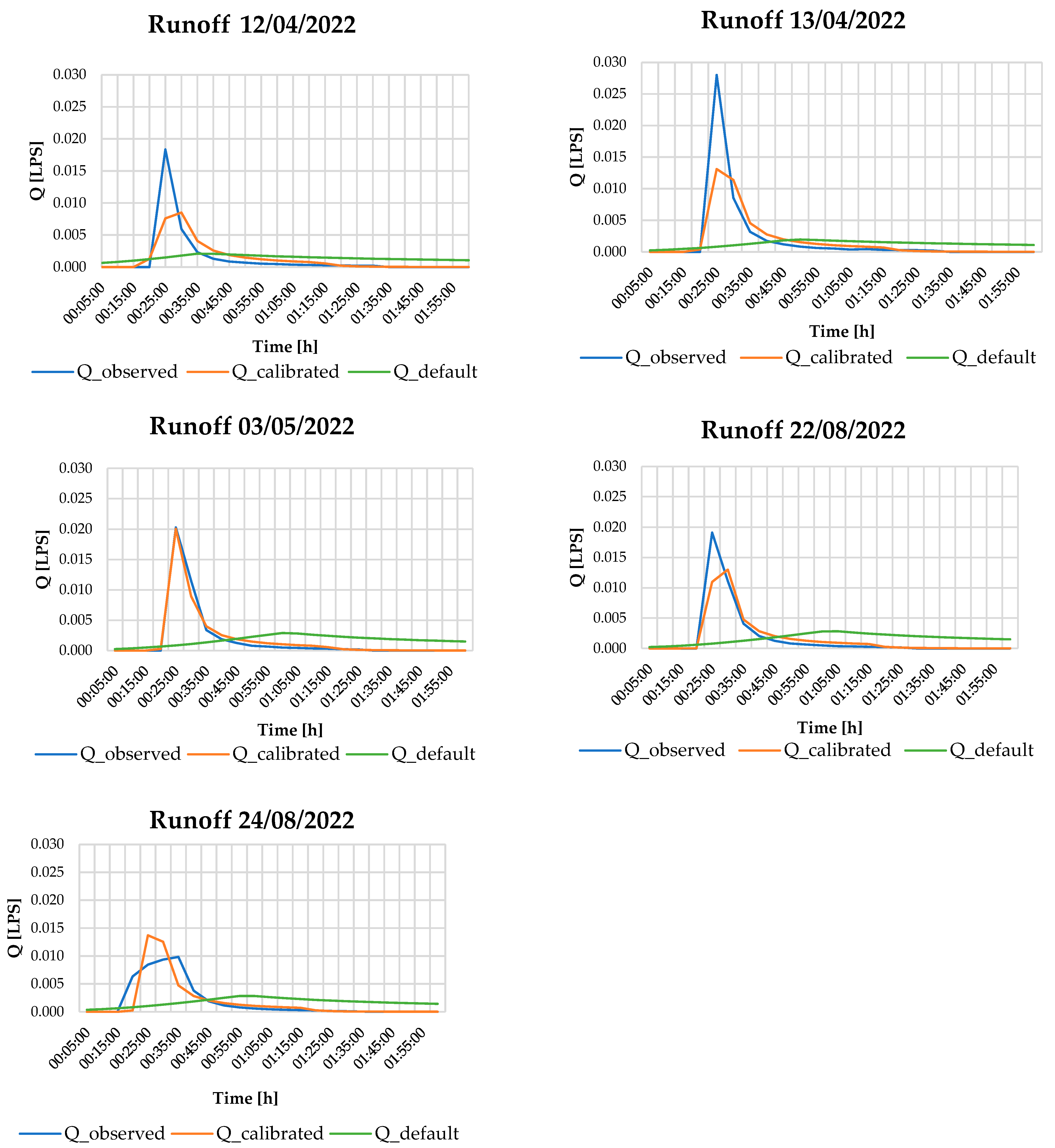
3.2. Comparison of Calibrated and Uncalibrated Model Results

A second, default model was run for five of the twenty-minute rainfall events, with their parameter settings shown in

Table 6. Differences in settings between the calibrated and default models.

Parameter (Units)	Calibrated	Default
Vegetation volume fraction (m3/m3)	0.1	0.0
Surface roughness (Mannings n)	0.1	0.1
Porosity (m3/m3)	0.457	0.5
Field capacity (m3/m3)	0.31	0.2
Wilting point (m3/m3)	0.004	0.1
Conductivity (mm/h)	5555	12.7
Conductivity slope (-)	53	10
Roughness drainage mat (Mannings n)	0.4	0.1

, to emphasize the importance of the calibration process. The NSE and VE scores are compared between both models and presented in

Table 7. NSE and VE scores: comparison of the calibrated and uncalibrated models.

Date	Calibrated		Default
	NSE	VE	NSE	VE
12-04-22	0.61	0.88%	0.15	67.52%
13-04-22	0.70	10.71%	0.05	50.19%
03-05-22	0.98	2.98%	−0.11	58.81%
22-08-22	0.83	2.49%	−0.13	63.65%
24-08-22	0.76	1.68%	−0.03	61.41%

.

There were significant differences between NSE results and the volume error for the calibrated and uncalibrated models. The mean NSE and VE of these events without calibration were −0.014 and 60.3%, respectively. These results were classified as unsatisfactory. With calibration, the mean NSE and VE of these events improved to 0.78 and 3.8%, respectively.

An improvement in the results after the calibration of the SWMM for green roofs was also verified in the study by Hamouz and Muthana [52], who observed an improvement in NSE from 0.44 to 0.88 after calibration.

In Figure 6, the experimentally observed runoff, the runoff resulting from the calibrated model, and the runoff resulting from the model with default settings of the five events are presented.

A comparison of the graphs and the previous results reveals that the peak flows of the default model are much lower and later in time than those observed in field measurements. This means that, in this case, the default model overestimated the hydraulic performance of the green roofs. These differences likely resulted from differences in porosity, wilting point, and field capacity.

The wilting point is defined as the amount of water in the soil, expressed as a ratio, which cannot be absorbed by the plants because it is being held very tightly by the soil. The wilting point is dependent on several variables, including the plant type. A higher wilting point leads to higher runoff volume and runoff peak flow, and consequently to lower hydraulic efficiency of the green roof. In the model with default settings, the wilting point was higher than the calibrated model, which would impair its hydraulic performance [43].

Field capacity is the volume of pore water relative to the total volume after the soil has fully drained. Below this level, the vertical drainage of water through the soil layer does not occur [43]. Therefore, a higher field capacity leads to a higher retention capacity and thus a better hydraulic performance of the green roof. After calibration, a field capacity of 0.31 was found, closer to the maximum limit, instead of 0.2 of the SWMM default settings, which would result in a lower performance.

This being the case, the main parameter causing this overestimation is likely to be the porosity, which is directly related to the field capacity, which was found to be a sensitive parameter during the calibration process. As shown in Table 6, the porosity has a higher value in the default model. A higher porosity value helps to increase the hydraulic performance of green roofs since it has more voids available to be filled by water in rainfall events.

In the literature, different results have been found in studies that have also compared the performance of a calibrated model with an uncalibrated one [21,22]. While Rosa et al. [21] concluded that the runoff simulated using the uncalibrated model was underestimated, Iffland et al. [22] revealed that the results of their default model overestimated the runoff. It should also be noted that Iffland et al. [22] used different parameter values for their default model. Instead of taking the values pre-filled by the SWMM, they based their default settings on a parameter range provided by Krebs et al. [26], in combination with the SWMM Reference Manual [43]. This includes parameters that were considered in their sensitivity analysis.

In summary, although the default model in this research showed a higher wilting point value and a lower field capacity value, which could impair the hydraulic performance of green roofs, the results showed that its runoff volume and runoff peak flow were lower than those of the calibrated model. Thus, this overestimation of the hydraulic performance of the model is attributed to the porosity parameter, which was higher in the default model than in the calibrated model, in which a value measured in the field was used.

The results found here demonstrate that the SWMM green roof module, if properly calibrated, can be successfully used to predict the hydraulic behavior of green roofs with known physical measurements. Palla and Gnecco [54] and Peng and Stovin [25] reached the same conclusion in their study. However, they also pointed out that, although their calibration results are reasonable, the calibrated parameters are only valid for a green roof that has the same characteristics as the one used in their study.

By comparing both models with the observed runoff, it became clear that calibration is necessary to obtain reliable model predictions. When using the suggested parameter values of the SWMM, the model in this case overestimated the performance of green roofs.

This research stresses the need for calibration and serves as a warning to practitioners about the potential large discrepancies when using default settings, in terms of risks of under-sizing green roof volumes, particularly in the Mediterranean climate. As emphasized by Niazi et al. [55], the lack of guidance on parameter estimation is still a shortcoming of the SWMM, and special attention should be paid to this aspect.

In addition, the LID parameter values found in this research can serve as points of reference for practitioners in the field.

4. Conclusions

In this paper, we evaluated the accuracy of the latest version of the SWMM 5.2 software for modeling the hydraulic performance of green roofs. For this, two campaigns of experiments with artificial rainfall were performed on pilot green roofs, installed in Lisbon, Portugal.

The calibrated model was able to simulate the runoff with a very good fit, having NSE values up to 0.91 and VE as small as 0.18%. The uncalibrated model performed poorly, with the mean NSE and VE being −0.014 and 60.3%, respectively. From this, it can be concluded that a calibration process is necessary for proper model predictions. The results of the uncalibrated model were, in general, overestimated if compared to the results observed in the experimental tests. The parameter that seems to have the greatest influence on the final result is the field capacity/porosity, which had a higher value for the model with the default settings.

Thus, the need for the calibration of the SWMM for projects and decision making is highlighted. In this case, predictions of the uncalibrated default model showed a significantly stronger decrease in peak flow than what occurs in reality.

For future studies, the use of continuous real rainfall events is recommended, so that a simulated pre-rainfall step would not be needed, which the necessity of this step was a limitation of this research. In addition, using large-scale green roofs is also recommended, to better understand the possibility of upscaling the calibrated model.

References

1. Brandão, C.; Cameira, M.d.R.; Valente, F.; Cruz de Carvalho, R.; Paço, T.A. Wet season hydrological performance of green roofs using native species under Mediterranean climate. Ecol. Eng. 2017, 102, 596–611. [Google Scholar] [CrossRef]
2. Fletcher, T.D.; Shuster, W.; Hunt, W.F.; Ashley, R.; Butler, D.; Arthur, S.; Viklander, M. SUDS, LID, BMPs, WSUD and more—The evolution and application of terminology surrounding urban drainage. Urban Water J. 2015, 12, 525–542. [Google Scholar] [CrossRef]
3. Orta-Ortiz, M.S.; Geneletti, D. What variables matter when designing nature-based solutions for stormwater management? A review of impacts on ecosystem services. Environ. Impact Assess. Rev. 2022, 95, 106802. [Google Scholar] [CrossRef]
4. Carson, T.B.; Marasco, D.E.; Culligan, P.J.; McGillis, W.R. Hydrological performance of extensive green roofs in New York City: Observations and multi-year modeling of three full-scale systems. Environ. Res. Lett. 2013, 8, 13. [Google Scholar] [CrossRef]
5. Manso, M.; Teotónio, I.; Silva, C.M.; Cruz, C.O. Green roof and green wall benefits and costs: A review of the quantitative evidence. Renew. Sustain. Energy Rev. 2021, 135, 110111. [Google Scholar] [CrossRef]
6. Zhang, Z.; Liu, D.; Zhang, R.; Li, J.; Wang, W. The impact of rainfall change on rainwater source control in Beijing. Urban Clim. 2021, 37, 100841. [Google Scholar] [CrossRef]
7. Qin, H.P.; Li, Z.X.; Fu, G. The effects of low impact development on urban flooding under different rainfall characteristics. J. Environ. Manag. 2013, 129, 577–585. [Google Scholar] [CrossRef]
8. Eksi, M.; Rowe, D.B. Green roof substrates: Effect of recycled crushed porcelain and foamed glass on plant growth and water retention. Urban For. Urban Green. 2016, 20, 81–88. [Google Scholar] [CrossRef]
9. Schultz, I.; Sailor, D.J.; Starry, O. Effects of substrate depth and precipitation characteristics on stormwater retention by two green roofs in Portland OR. J. Hydrol. Reg. Stud. 2018, 18, 110–118. [Google Scholar] [CrossRef]
10. Soulis, K.X.; Ntoulas, N.; Nektarios, P.A.; Kargas, G. Runoff reduction from extensive green roofs having different substrate depth and plant cover. Ecol. Eng. 2017, 102, 80–89. [Google Scholar] [CrossRef]
11. Hakimdavar, R.; Culligan, P.J.; Finazzi, M.; Barontini, S.; Ranzi, R. Scale dynamics of extensive green roofs: Quantifying the effect of drainage area and rainfall characteristics on observed and modeled green roof hydrologic performance. Ecol. Eng. 2014, 73, 494–508. [Google Scholar] [CrossRef]
12. Alfredo, K.; Montalto, F.; Goldstein, A. Observed and Modeled Performances of Prototype Green Roof Test Plots Subjected to Simulated Low- and High-Intensity Precipitations in a Laboratory Experiment. J. Hydrol. Eng. 2010, 15, 444–457. [Google Scholar] [CrossRef]
13. Stovin, V.; Vesuviano, G.; Kasmin, H. The hydrological performance of a green roof test bed under UK climatic conditions. J. Hydrol. 2012, 414–415, 148–161. [Google Scholar] [CrossRef]
14. Johannessen, B.G.; Hamouz, V.; Gragne, A.S.; Muthanna, T.M. The transferability of SWMM model parameters between green roofs with similar build-up. J. Hydrol. 2019, 569, 816–828. [Google Scholar] [CrossRef]
15. Cipolla, S.S.; Maglionico, M.; Stojkov, I. A long-term hydrological modelling of an extensive green roof by means of SWMM. Ecol. Eng. 2016, 95, 876–887. [Google Scholar] [CrossRef]
16. Santos, M.L.; Silva, C.M.; Ferreira, F.; Matos, J.S. Hydrological Analysis of Green Roofs Performance under a Mediterranean Climate: A Case Study in Lisbon, Portugal. Sustainability 2023, 15, 1064. [Google Scholar] [CrossRef]
17. Stovin, V.; Vesuviano, G.; De-Ville, S. Defining green roof detention performance. Water J. 2015, 14, 574–588. [Google Scholar] [CrossRef]
18. Czemiel Berndtsson, J. Green roof performance towards management of runoff water quantity and quality: A review. Ecol. Eng. 2010, 36, 351–360. [Google Scholar] [CrossRef]
19. Jeffers, S.; Garner, B.; Hidalgo, D.; Daoularis, D.; Warmerdam, O.; Warmerdam, O. Insights into green roof modeling using SWMM LID controls for detention-based designs. Artic. J. Water Manag. Model. 2022, 30, 484. [Google Scholar] [CrossRef]
20. Burszta-Adamiak, E.; Mrowiec, M. Modelling of green roofs’ hydrologic performance using EPA’s SWMM. Water Sci. Technol. 2013, 68, 36–42. [Google Scholar] [CrossRef]
21. Rosa, D.J.; Clausen, J.C.; Dietz, M.E. Calibration and Verification of SWMM for Low Impact Development. JAWRA J. Am. Water Resour. Assoc. 2015, 51, 746–757. [Google Scholar] [CrossRef]
22. Iffland, R.; Förster, K.; Westerholt, D.; Pesci, M.H.; Lösken, G. Robust vegetation parameterization for green roofs in the EPA stormwater management model (SWMM). Hydrology 2021, 8, 12. [Google Scholar] [CrossRef]
23. Worthen, L.L.; Davidson, C.I. Sensitivity Analysis Using the SWMM LID Control for an Extensive Green Roof in Syracuse, NY. In Proceedings of the 7th International Building Physics Conference, IBPC2018, Syracuse, NY, USA, 23–26 September 2018. [Google Scholar]
24. Limos, A.G.; Mallari, K.J.B.; Baek, J.; Kim, H.; Hong, S.; Yoon, J. Assessing the significance of evapotranspiration in green roof modeling by SWMM. J. Hydroinform. 2018, 20, 588–596. [Google Scholar] [CrossRef]
25. Peng, Z.; Stovin, V. Independent Validation of the SWMM Green Roof Module. J. Hydrol. Eng. 2017, 22, 04017037. [Google Scholar] [CrossRef]
26. Krebs, G.; Kuoppamäki, K.; Kokkonen, T.; Koivusalo, H. Simulation of green roof test bed runoff. Hydrological processes. Hydrol. Process. 2016, 30, 250–262. [Google Scholar] [CrossRef]
27. Paithankar, D.N.; Taji, S.G. Investigating the hydrological performance of green roofs using storm water management model. Mater. Today Proc. 2020, 32, 943–950. [Google Scholar] [CrossRef]
28. Palermo, S.A.; Turco, M.; Principato, F.; Piro, P. Hydrological effectiveness of an extensive green roof in Mediterranean climate. Water 2019, 11, 1378. [Google Scholar] [CrossRef]
29. Cristiano, E.; Urru, S.; Farris, S.; Ruggiu, D.; Deidda, R.; Viola, F. Analysis of potential benefits on flood mitigation of a CAM green roof in Mediterranean urban areas. Build. Environ. 2020, 183, 107179. [Google Scholar] [CrossRef]
30. Fioretti, R.; Palla, A.; Lanza, L.G.; Principi, P. Green roof energy and water related performance in the Mediterranean climate. Build. Environ. 2010, 45, 1890–1904. [Google Scholar] [CrossRef]
31. Razzaghmanesh, M.; Beecham, S. The hydrological behaviour of extensive and intensive green roofs in a dry climate. Sci. Total Environ. 2014, 499, 284–296. [Google Scholar] [CrossRef]
32. Buccola, N.; Spolek, G. A pilot-scale evaluation of greenroof runoff retention, detention, and quality. Water Air Soil Pollut. 2011, 216, 83–92. [Google Scholar] [CrossRef]
33. Piro, P.; Carbone, M.; De Simone, M.; Maiolo, M.; Bevilacqua, P.; Arcuri, N. Energy and Hydraulic Performance of a Vegetated Roof in Sub-Mediterranean Climate. Sustainability 2018, 10, 3473. [Google Scholar] [CrossRef]
34. Doménech, I.; Perales-Momparler, S.; Morales-Torres, A.; Escuder-Bueno, I. Hydrological Performance of Green Roofs at Building and City Scales under Mediterranean Conditions. Sustainability 2018, 10, 3105. [Google Scholar] [CrossRef]
35. Palla, A.; Sansalone, J.J.; Gnecco, I.; Lanza, L.G. Storm water infiltration in a monitored green roof for hydrologic restoration. Water Sci. Technol. 2011, 64, 766–773. [Google Scholar] [CrossRef] [PubMed]
36. Schroll, E.; Lambrinos, J.; Righetti, T.; Sandrock, D. The role of vegetation in regulating stormwater runoff from green roofs in a winter rainfall climate. Ecol. Eng. 2011, 37, 595–600. [Google Scholar] [CrossRef]
37. Rocha, B.; Paço, T.A.; Luz, A.C.; Palha, P.; Milliken, S.; Kotzen, B.; Branquinho, C.; Pinho, P.; de Carvalho, R.C. Are biocrusts and xerophytic vegetation a viable green roof typology in a mediterranean climate? A comparison between differently vegetated green roofs in water runoff and water quality. Water 2021, 13, 94. [Google Scholar] [CrossRef]
38. Barnhart, B.; Pettus, P.; Halama, J.; McKane, R.; Mayer, P.; Djang, K.; Brookes, A.; Moskal, L.M. Modeling the hydrologic effects of watershed-scale green roof implementation in the Pacific Northwest, United States. J. Environ. Manag. 2021, 277, 111418. [Google Scholar] [CrossRef] [PubMed]
39. Garofalo, G.; Palermo, S.; Principato, F.; Theodosiou, T.; Piro, P. The Influence of Hydrologic Parameters on the Hydraulic Efficiency of an Extensive Green Roof in Mediterranean Area. Water 2016, 8, 44. [Google Scholar] [CrossRef]
40. Rossman, L.; Huber, W. Storm Water Management Model Reference Manual Volume I, Hydrology. USEPA Office of Research and Development. Washington 2015, DC. EPA/600/R-15/162A. Available online: https://nepis.epa.gov/Exe/ZyPURL.cgi?Dockey=P100NYRA.Txt (accessed on 5 June 2023).
41. Rossman, L.A. Storm Water Management Model User’s Manual Version 5.0. EPA/600/R-05/040; US EPA National Risk Management Research Laboratory: Cincinnati, OH, USA, 2010. [Google Scholar]
42. Chapra, S.C. Surface Water-Quality Modeling; Waveland Press: Long Grove, IL, USA, 1997; pp. 327–341. [Google Scholar]
43. Rossman, L.A. Storm Water Management Model User’s Manual Version 5.2. EPA/600/R-22/030; US EPA National Risk Management Research Laboratory: Cincinnati, OH, USA, 2022. [Google Scholar]
44. Leimgruber, J.; Krebs, G.; Camhy, D.; Muschalla, D. Sensitivity of model-based water balance to low impact development parameters. Water 2018, 10, 1838. [Google Scholar] [CrossRef]
45. ZinCo, I. Cobertura Ecológica Extensiva “Tapete Sedum”. 2022. Available online: https://zinco.pt/sistemas/extensivas/tapete_sedum.php (accessed on 21 August 2023).
46. IPMA. Boletim Anual 2022. Available online: https://www.ipma.pt/resources.www/docs/im.publicacoes/edicoes.online/20230328/RLuazVlyZulVPByQUNey/cli_20220101_20221231_pcl_aa_co_pt.pdf (accessed on 2 July 2023).
47. Pordata. Available online: https://www.pordata.pt/db/portugal/ambiente+de+consulta/tabela (accessed on 5 July 2023).
48. Regulatory Decree nº 23/95-Regulamento Geral dos Sistemas Públicos e Prediais de Distribuição de Água e de Drenagem de Águas Residuais, Portugal, August 1995. Available online: https://diariodarepublica.pt/dr/detalhe/decreto-regulamentar/23-1995-431873 (accessed on 21 August 2023).
49. Ferreira, F. Modelação e Gestão Integrada de Sistemas de Águas Residuais. Dissertação de Doutoramento em Engenharia Civil, IST/UNL, Lisboa, Portugal, 2006. [Google Scholar]
50. Hossain, S.; Hewa, G.A.; Wella-Hewage, S. A Comparison of Continuous and Event-Based Rainfall–Runoff (RR) Modelling Using EPA-SWMM. Water 2019, 11, 611. [Google Scholar] [CrossRef]
51. Moriasi, D.N.; Arnold, J.G.; Van Liew, M.W.; Bingner, R.L.; Harmel, R.D.; Veith, T.L. Model evaluation guidelines for systematic quantification of accuracy in watershed simulations. Trans. ASABE 2007, 50, 885–900. [Google Scholar] [CrossRef]
52. Hamouz, V.; Muthanna, T.M. Hydrological modelling of green and grey roofs in cold climate with the SWMM model. J. Environ. Manag. 2019, 249, 109350. [Google Scholar] [CrossRef] [PubMed]
53. Arjenaki, M.O.; Sanayei, H.; Heidarzadeh, H.; Mahabadi, N. Modeling and investigating the effect of the LID methods on collection network of urban runoff using the SWMM model (case study: Shahrekord City). Model. Earth Syst. Environ. 2021, 7, 1–16. [Google Scholar] [CrossRef]
54. Palla, A.; Gnecco, I. Hydrologic modeling of Low Impact Development systems at the urban catchment scale. J. Hydrol. 2015, 528, 361–368. [Google Scholar] [CrossRef]
55. Niazi, M.; Nietch, C.; Maghrebi, M.; Jackson, N.; Bennett, B.R.; Tryby, M.; Massoudieh, A. Storm water management model: Performance review and gap analysis. J. Sustain. Water Built Environ. 2017, 3, 04017002. [Google Scholar] [CrossRef]
Figure 1. The conceptual model of the green roof LID control in SWMM 5.2.
Sustainability 15 14421 g001
Figure 2. Consecutive steps of the research methodology.
Sustainability 15 14421 g002
Figure 3. Artificial rainfall intensity of the second campaign in April 2023.
Sustainability 15 14421 g003
Figure 4. Intensity–duration–frequency curves for low rainfall intensities in Lisbon (adapted from Ferreira [49]).
Sustainability 15 14421 g004
Figure 5. Artificial rainfall system installed on the test-bed pilot units.
Sustainability 15 14421 g005
Figure 6. Hydrographs with observed runoff, calibrated model runoff, and default model runoff.
Sustainability 15 14421 g006