Examination of Single- and Hybrid-Based Metaheuristic Algorithms in ANN Reference Evapotranspiration Estimating

Abstract

Hydrological resource management, including crop watering and irrigation scheduling, relies on reliable estimates of reference evapotranspiration (ETo). However, previous studies of forecasting ETo have not dealt with comparing single and hybrid metaheuristic algorithms in much detail. This study aims to assess the efficiency of a novel methodology to simulate univariate monthly ETo estimates using an artificial neural network (ANN) integrated with the hybrid particle swarm optimisation–grey wolf optimiser algorithm (PSOGWO). Several state-of-the-art algorithms, including constriction coefficient-based particle swarm optimisation and chaotic gravitational search algorithms (CPSOCGSA), the slime mould algorithm (SMA), the marine predators algorithm (MPA) and the modified PSO algorithm were used to evaluate PSOGWO’s prediction accuracy. Monthly meteorological data were collected in Al-Kut City (1990 to 2020) and used for model training, testing and validation. The results indicate that pre-processing techniques can improve raw data quality and may also suggest the best predictors scenario. That said, all models can be considered efficient with acceptable simulation levels. However, the PSOGWO-ANN model slightly outperformed the other techniques based on several statistical tests (e.g., a coefficient of determination of 0.99). The findings can contribute to better management of water resources in Al-Kut City, an agricultural region that produces wheat in Iraq and is under the stress of climate change.

1. Introduction

1.1. Research Background

Water scarcity is a growing issue, especially in arid and semi-arid regions [1], because it endangers the sustainability of food production systems and creates worries around food security [2]. The major consumer of freshwater resources worldwide is agriculture [3]. By 2050, there will be a 60% increase in the world’s food needs [4], meaning that informed and careful management of irrigation practices will be required and could result in substantial water savings [5]. Reference evapotranspiration (ETo) is a crucial part of the hydrological cycle; its fluctuations are relevant for managing water resources, irrigation scheduling and agricultural yield [6]. The existing literature suggests that the preferred approach for calculating ETo is the FAO Penman–Monteith equation (FAO-56 PM) [7]. However, the FAO-56 PM technique is less adaptable and difficult to apply to diverse climate circumstances, primarily arid and semi-arid countries, because it requires many meteorological factors that might not be available, similar to many other empirical models [8].

Iraq’s main sources of fresh water are the Tigris and Euphrates rivers. These rivers originate in Turkey, Syria and Iran. Consequently, Iraq’s water supplies have been affected by both climate change and human-induced interventions upstream (i.e., unilateral damming, water abstraction and inter-basin water transfer schemes in the upper riparian nations, mainly Turkey and Iran). Therefore, Iraq is confronted with increasing difficulties in managing its water supplies. Droughts that last for months at a time have become all too prevalent in Iraq [9,10]. Also, due to rising temperatures, insufficient and decreasing rainfall, lengthy droughts and water scarcity, frequent sand and dust storms and flooding, Iraq has been ranked as the fifth most vulnerable country to climate change and the thirty-ninth most water-stressed [11].

1.2. Applied Machine Learning Methods for ETo Forecasting

Irrigation planning can benefit from not only past and present ETo estimations, but also future ETo forecasts [12]. Recently, machine learning (ML) methods have been effectively applied to predict ETo in different regions [13,14]. On the basis of monthly lagged meteorological data Nourani et al. [1], anticipated ETo up to 3 months in advance. Artificial neural networks (ANN), support vector machines (SVM) and adaptive neuro-fuzzy inference systems (ANFIS) were used singly and multimodally to achieve this. The outputs of separate models were fed into the weighted average (WA), simple average (SA) and neural ensemble (NE) techniques. Monthly meteorological parameters from a number of weather stations in Iraq, North Cyprus and Turkey were employed as input during the creation of the models. Due to their linear behaviour, SA and WA ensembles did not exhibit a substantial increase in performance, but WA was found to be superior to SA. NE performed the best across all stations and modelling processes. The overall outcomes confirmed that the multimodal strategy performed better than single techniques, boosting performance up to 24%, 33% and 60% for stations in Iraq, North Cyprus and Turkey, respectively.

Ferreira and da Cunha [12] worked on predicting daily multi-step (7 days) ETo. They used the potential of traditional ML methods (ANN and random forest (RF)) and deep learning (DL) models (long short-term memory (LSTM), one-dimensional convolutional neural networks (1D CNN)) and a hybrid of the two previous techniques (CNN-LSTM), in local and regional scenarios. Fifty-three automated weather stations in Brazil were used, and their results revealed that DL techniques outperformed ML methods by a small margin, CNN-LSTM2 and CNN-LSTM3 achieving the best results.

Sayyahi et al. [15] simulated daily and monthly ETo with lags of one, two and three days, and one, two and three months, at the Aidoghmoush Basin, Iran. They integrated the multilayer perceptron (MLP) model with three metaheuristic algorithms (MHAs), including water wave optimisation (WWO), genetic algorithm (GA) and particle swarm optimisation (PSO). The MLP-WWO outputs were more in line with the data that was actually observed, outperforming MLP, MLP-PSO and MLP-GA techniques.

1.3. Research Significance and Motivation

Traditional ML approaches, such as ANN, SVM and ANFIS, are also applied to estimate ETo. However, complex, non-linear and high-dimensional computing issues make it difficult to find global optimum solutions, and the number of possible solutions may be infinite. It is crucial to find a workable answer in such predicaments [16]. Metaheuristic optimisation algorithms (MHAs) have proven to be effective in tackling a wide range of non-linear and difficult problems in various domains of hydrology (i.e., when hybrid models are compared with standalone ML models), such as [17,18,19]. These hybrid models are preferable for tackling complex practical problems [20]. Because of this, these techniques have demonstrated success in locating novel areas that may increase the breadth of possible solutions [21]. Additionally, the capacity for exploitation is enhanced in order to prevent being stuck in local minima. In conclusion, these techniques are superior in their ability to handle nonlinearity, multi-variable and complicated situations [22].

According to the “no free lunch” theorem, there is no optimal solution for resolving all possible optimisation problems [23]. Another way of saying this is that there is no such thing as an optimal optimisation procedure that can be applied in all cases. Because of this, scientists in a wide variety of fields are more motivated to design novel algorithms (single-based) or develop hybrid algorithms (hybrid-based) in order to tackle increasingly difficult issues with high dimensionalities [16,24].

Metaheuristic optimisation algorithms have become increasingly popular and are used to develop hybrid models for hydrological research, such as ETo prediction [25]. MHAs seek the best viable answer within an optimisation problem [26,27]. Amongst these algorithms is the slime mould algorithm (SMA), which was introduced by Li et al. [28].

SMA imitates the slime mould Physarum polycephalum’s structural and performance fluctuations whilst it is seeking nourishment [29]. It has been used to address various optimisation difficulties, including issues with engineering designs [30] and estimation of the characteristics of solar photovoltaic cells [31]. Faramarzi et al. [32] developed the marine predators algorithm (MPA), which draws inspiration from nature and mimics predator behaviour when attacking prey. It has been employed in many fields, such as engineering applications [33] and sources of power [34]. The constriction coefficient-based particle swarm optimisation and chaotic gravitational search algorithm (CPSOCGSA), was developed by Rather and Bala [35]. It was created by merging the PSO method, which simulates the behaviour of flocks of birds, with the gravitational search algorithm (GSA), as an application of Newton’s law of universal gravity.

The above review of the literature demonstrates how optimisation methods can be used to strengthen predictor models [36], such as Tao et al. [37] and Maroufpoor et al. [38]. Optimisation algorithms’ primary strengths lie in their capacity to quickly and accurately determine the optimal settings of system parameters in response to changing conditions [39]. In spite of that, optimisation is still required, particularly in modelling hydrological variables like ETo, because of their stochastic, non-stationary nature and data noise [40].

MHAs primarily consist of two components: exploration and exploitation. “Exploration” is the process of determining the limits of an algorithm’s search space in computer science, while “exploitation” describes the selection of the optimal solution from the many possible generated [41]. A search algorithm needs to detect an optimal balance between exploration and exploitation in order to be effective [42]. Nevertheless, exploration and exploitation are inversely proportional to one another [43]. Along with creating new MHAs, another strategy is needed to combine the best features of several algorithms to create a superior algorithm. As a result, the hybrid particle swarm optimisation–grey wolf optimiser algorithm (PSOGWO), was developed by Şenel et al. [44]. It combines the exploitation capability of the PSO algorithm with the exploration capability of the grey wolf optimiser (GWO). Using the GWO algorithm’s exploration capability prevents the PSO algorithm from settling into local minimums, which can reduce the quality of the solution.

Recent research on the hybridisation of hybrid structures for time series forecasting by Hajirahimi and Khashei [45] showed the importance of pre-processing data and optimisation approaches. The hybridisation of hybrid techniques is a novel approach used to increase accuracy where two or more hybrid classes are fused, rather than the traditional combination of separate predicting approaches. One such tactic (HPOH) combines pre-processing-based and parameter optimisation-based hybrid techniques. There are, however, gaps in the research suggestive of future research related to the hybridisation of hybrid models.

Khairan et al. [17] reviewed the hybrid techniques (ML and MHAs) available to predict ETo. The hybrid techniques have been successfully applied to predicting ETo. Up to this point in time, far too little attention has been paid to hybrid-based MHAs (6%) compared with single-based MHAs. Accordingly, there is still room for development concerning ETo prediction models.

1.4. Research Objectives

Therefore, this study aims to integrate relatively recent hybrid-based MHAs with an ANN model to develop a strong combined technique to boost ETo forecasting accuracy. The primary objectives of this research are to:

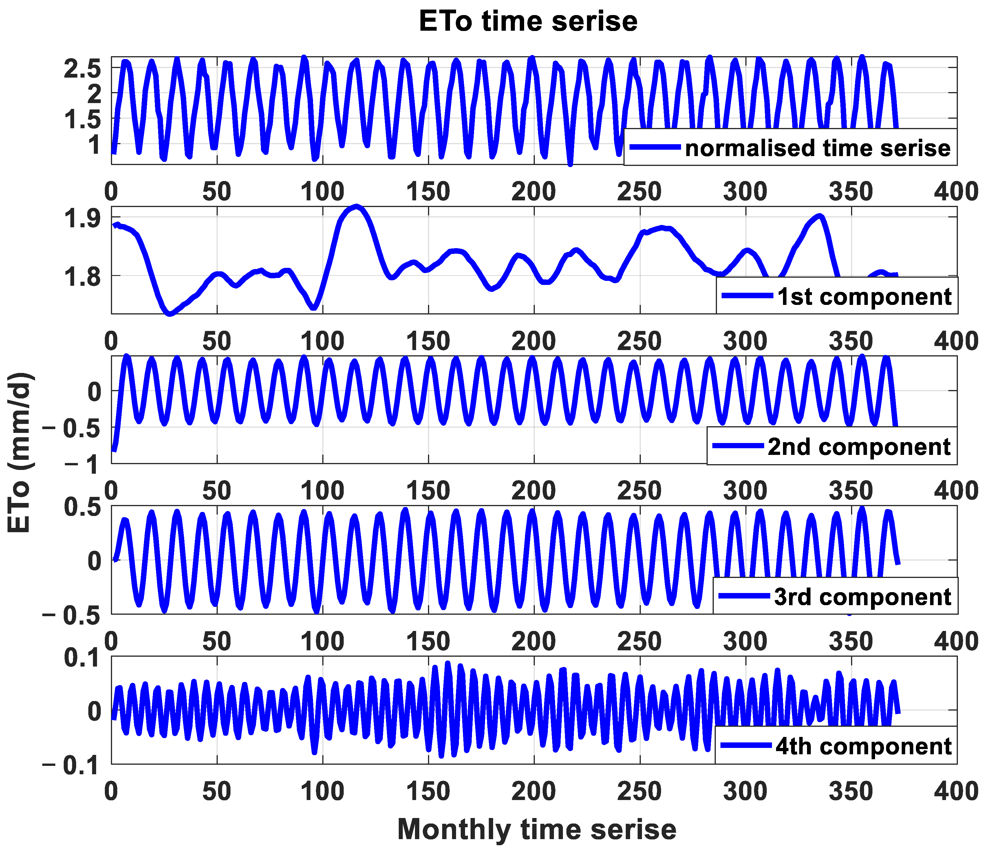
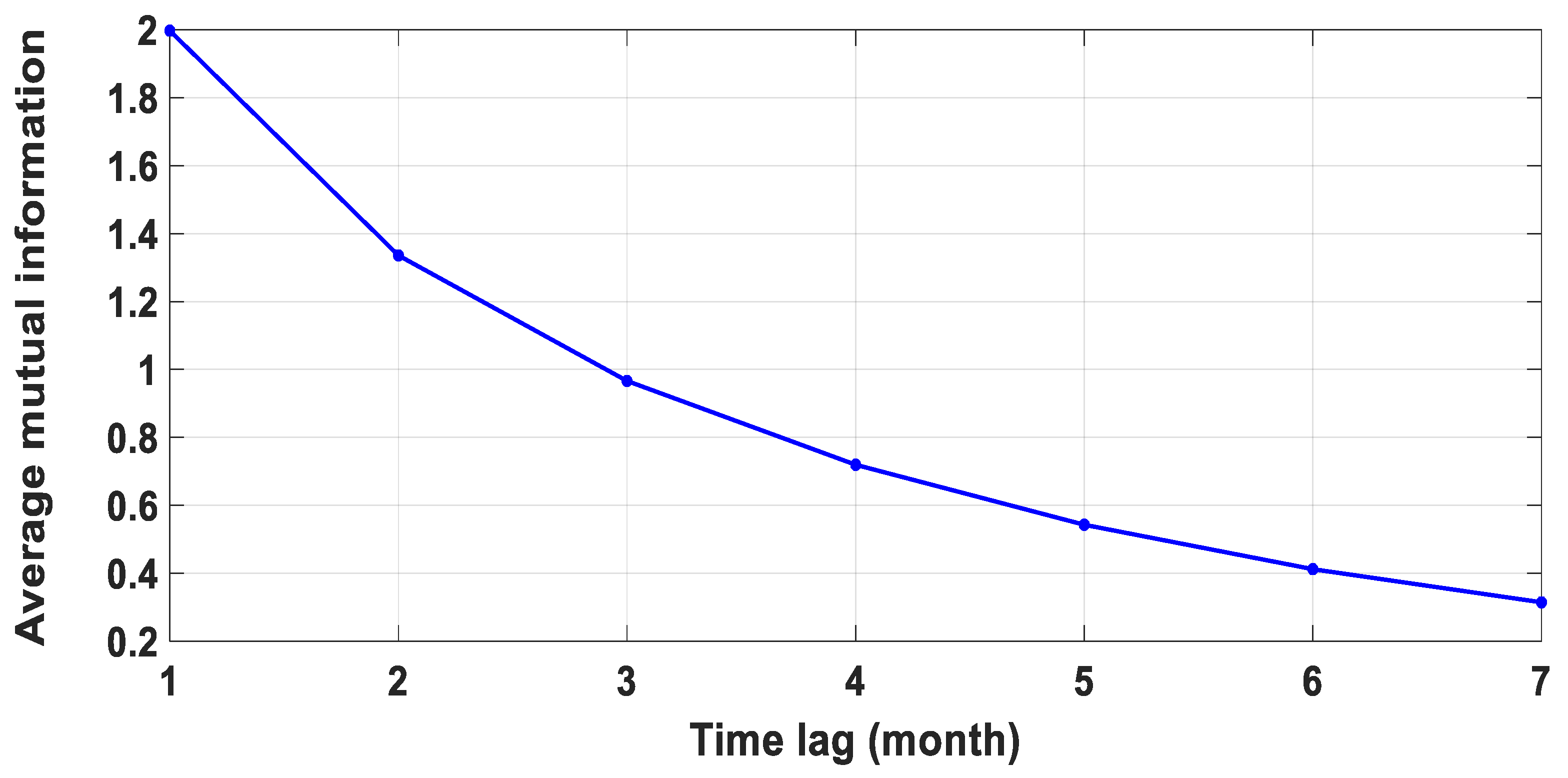
• Employ a pre-processing technique, namely singular spectrum analysis (SSA), to enhance the quality of the raw data and the mutual information (MI) technique to select the optimum model input (lags) scenario.
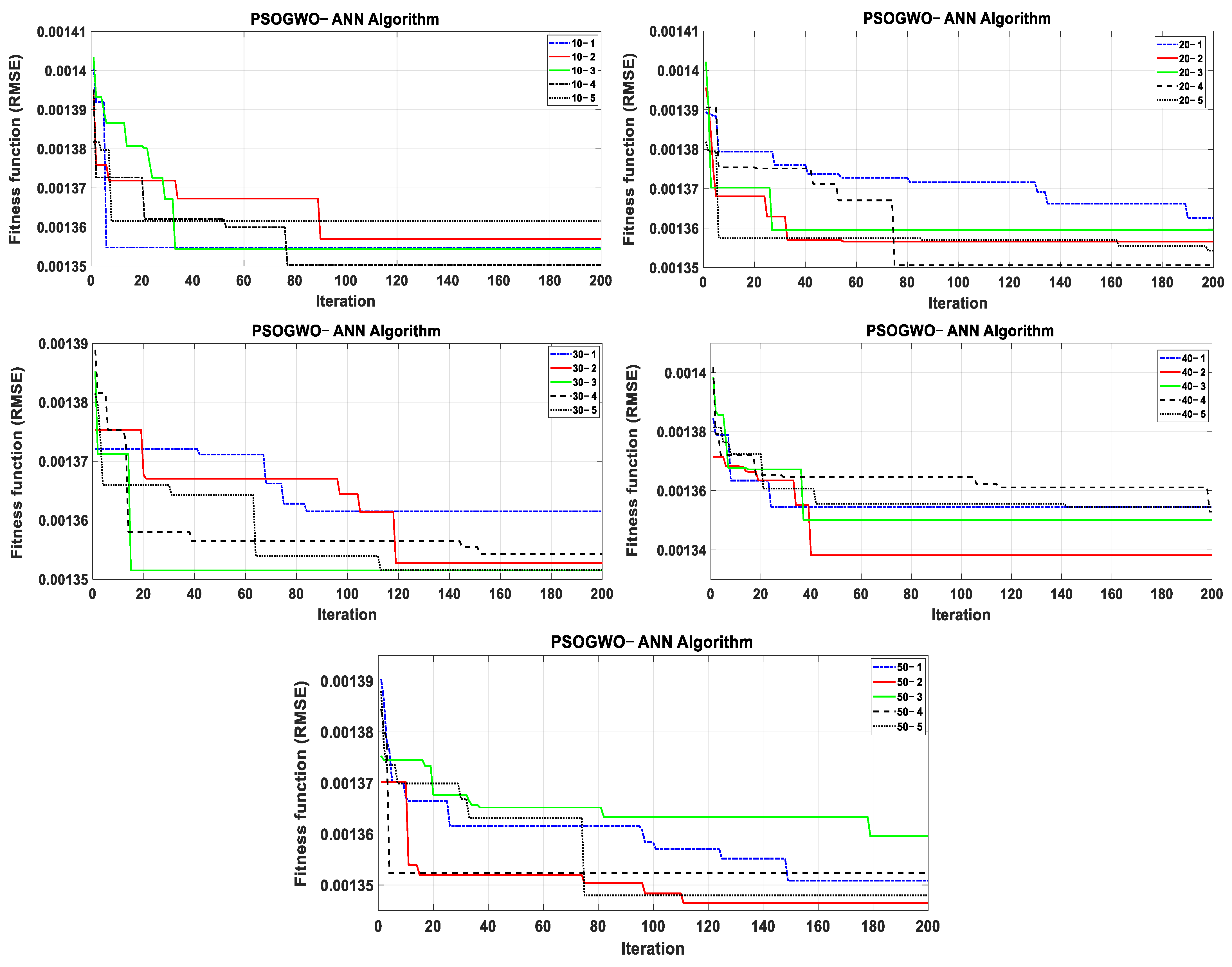
• Suggest a novel combined technique by coupling the ANN model with the hybrid-based PSOGWO algorithm to estimate monthly ETo based on multiple lags.
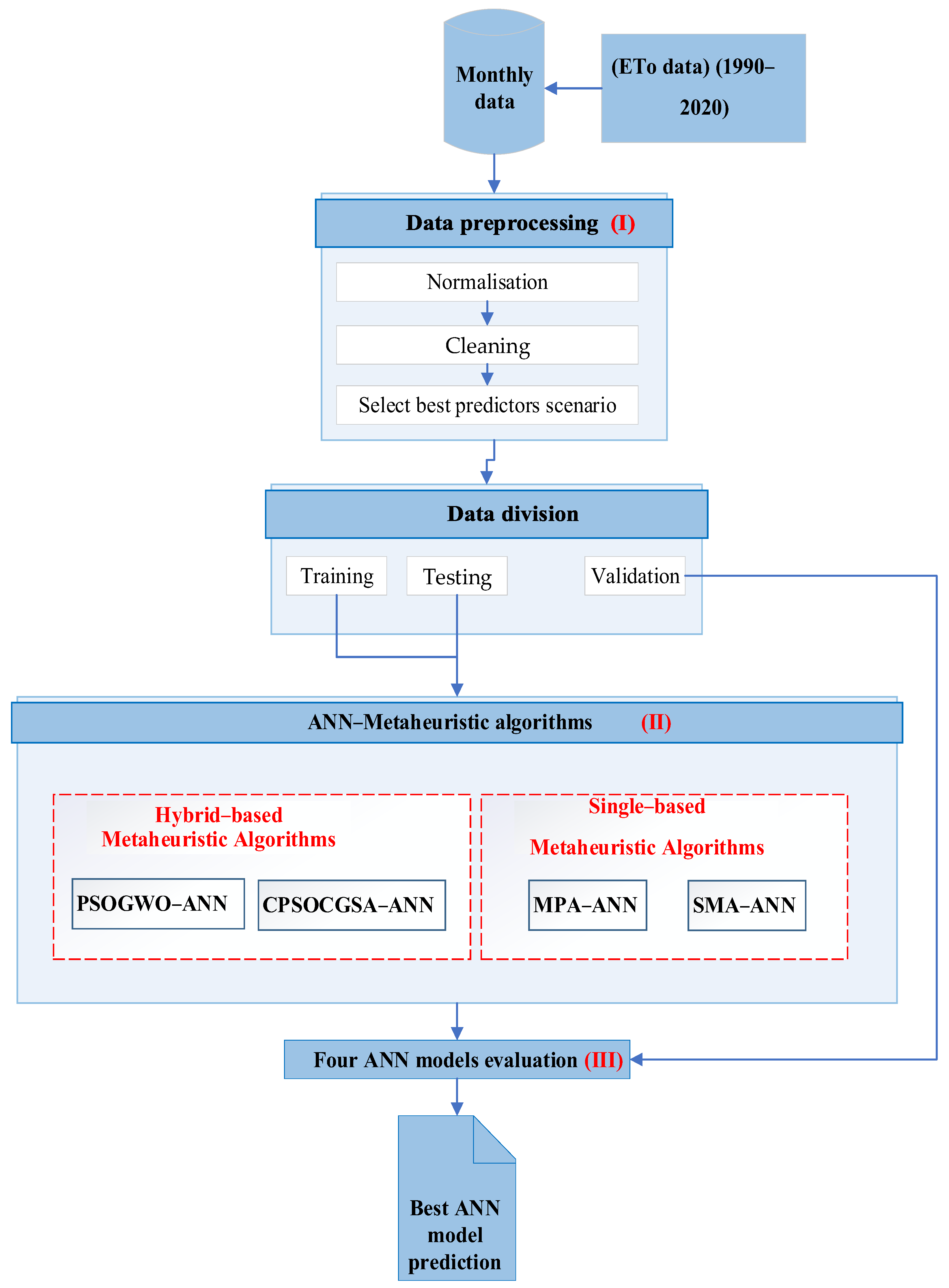
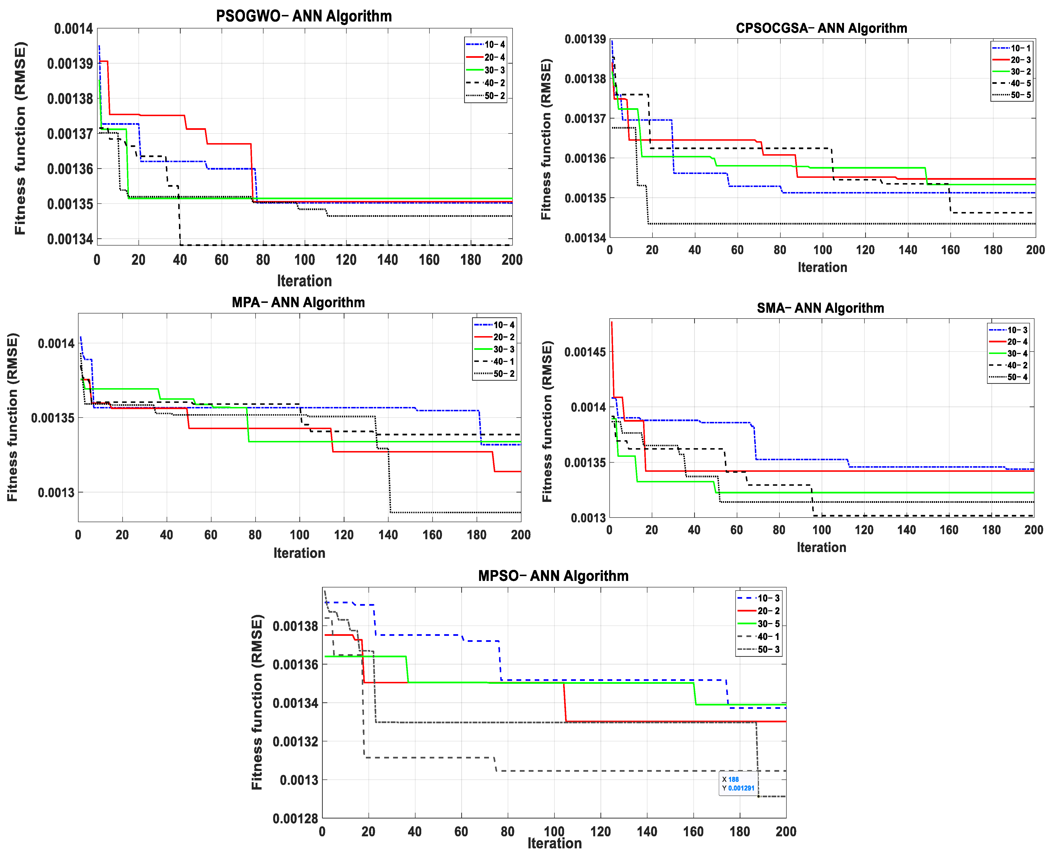
• Compare forecast accuracy and computational efficiency of the proposed PSOGWO-ANN model with other hybrid ML models, e.g., CPSOCGSA-ANN (hybrid-based), and single-based (i.e., MPA-ANN, SMA-ANN and MPSO-ANN).
• Examine how the novel HPOH technique simulates monthly ETo, depending on several lags.

2. Materials

2.1. Area of Study and Dataset

Iraq, located in the fastest-warming area of the world, faces temperatures up to 54 °C. It is experiencing significant effects of climate change, mainly drought, which results in decreased and altered precipitation patterns, as well as extreme heat waves [46]. The capital of Wasit Province, Al-Kut (Figure 1), which lies on the Tigris River in Southeastern Iraq [47], is approximately 40 square kilometres and is considered Iraq’s food basket [9]. The weather in Al-Kut City is considered normal but has short spring and fall seasons, approximately one month each, chilly in the winter and very dry and hot in the summer [48]. The Iraqi Meteorological Service states that the winter season officially starts in November and lasts until early March, the summer season lasting for most of the remaining months of the year, with June, July and August typically being the hottest months. Mean annual precipitation ranges between 150 and 300 mm [49].

Due to the water policies of Turkey and Iran, the Tigris River has reduced inflow by approximately two-thirds. Concurrent with changes in the oil industry that have increased the use of water, coupled with other socio-economic factors like the rapid population growth rate of about 2.5% that is taking place in Iraq, there are serious concerns with reference to the management of water resources [46].

The lack of meteorological data is a fundamental issue in developing nations. Due to exceptional circumstances, i.e., wars and terrorism in Iraq, most of the data from 1990–2020 are missing. Secondary (i.e., satellite) data offered by the National Aeronautics and Space Administration (NASA: Alawsi et al. [9] and Capt et al. [50]) were consequently used to carry out this study. These meteorological data were collected once a month over 30 years, between 1 January 1990 and 30 December 2020, comprising wind speed at the height of 2 m (U2) (m/s), relative humidity (RH) (percent), dew point temperature (Tdew) (°C), minimum temperature (Tmin) (°C), maximum temperature (Tmax) (°C) and solar radiation (Rs) (MJ/m²/day). The meteorological parameters are described statistically in

Table 1. The statistical parameters of the meteorological time series.

Variable	Mean	Maximum	Minimum
U2	1.83	5.34	3.0497
RH	10.18	70.60	33.8648
Tdew	3.8761	12.05	−3.66
Tmin	17.9526	32.50	1.54
Tmax	32.6396	48.93	32.6396
Rs	19.3106	30.13	8.61

.

2.2. FAO-56 PM Approach

The FAO56-PM equation (Equation (1)) is applied to calculate ETo data, which are used to develop and assess the models under consideration. This equation was used because of its widespread application and good levels of performance [12].

$$ETo=\frac{0.408∆\left(Rn-G\right)+\gamma \frac{900}{Tave+273}U2(es-ea)}{∆+\gamma (1+0.34U2)}$$

(1)

where monthly ETo is measured by mm/day, Rn the net surface radiation (MJm⁻²day⁻¹), G the soil heat flux (MJm⁻²day⁻¹), Tave the average monthly temperature (°C), es the mean saturation vapour pressure (kPa), ea the actual vapour pressure (kPa), Δ the slope of vapour pressure function (kPa/°C) and γ the psychometric constant (kPa/°C). The FAO Irrigation and Drainage Paper No. 56 fully explains the method of calculation and ETo principles [51].

3. Methodology

This research suggests the following four techniques (Figure 2) for estimating ETo on a monthly basis, taking previous ETo data into account (i.e., univariate procedure). It consists of four stages: (I) data pre-processing techniques, (II) PSOGWO algorithm, (III) ANN model and (IV) model performance assessment. Detailed descriptions of different measures are provided below.

3.1. Data Pre-Processing Techniques

Before the training process, the data are normalised using a natural logarithm approach to make the data more static, reduce collinearity between predictors and increase the model’s precision and speed of fit [52,53]. The SSA approach is then used to denoise the normalised data. SSA is a strong method for data analysis applied to find important predictive properties for both linear and nonlinear time series [54]. It consists of two stages: first, the noise is eliminated, and then a new time series is reconstructed with less noise, after decomposing the original time series into various principal components (PCs), including trend, oscillatory components and irregular components [55]. By examining these elements, conclusions can be drawn about the properties of the original time series [56]. Mathematically, SSA can decompose a time series of n points into a number of components that are no more than half of n+1. Consequently, an analysis can begin with three PCs, gradually increasing the number until the best result is achieved [57]. Singular spectrum analysis is a useful method for separating a time series into its constituent principal components (PCs). The first PC has the highest value, and the last PC has the lowest value in explaining the variance of the original time series. By focusing on the PCs that contribute the most variance and ignoring the PCs that contribute the least, SSA can be used to remove the structureless noise present in a time series [58]. This method is beneficial in a number of domains, including drought estimating [59], hydrology [60] and stream flow forecasting [61].

Predictive ML models can be made more accurate with the use of an appropriate sequence of temporal delays (lags). On the other hand, models with insufficient or unnecessary lags may be inaccurate or overly complicated. Because of the need to assume linearity or heavy redundancy between lags, many optimal lag selection approaches underperform. To address the collinearity issue, this research also considered the average mutual information (AMI), which may be considered a nonlinear generalisation of the autocorrelation function [62]. The MI method is used in this research to select the best explanatory factors. It calculates the statistical correlation between the target and lag data, thereby allowing the choice of the highest correlation components with the most MI [63]. The SPSS 24 statistics package was used to implement the normalisation and select the best predictor stages, while the MATLAB (version 2023b) toolbox was applied to perform the SSA algorithm.

3.2. Hybrid Particle Swarm Optimisation–Grey Wolf Optimiser Algorithm (PSOGWO)

GWO is a MHAs created by Mirjalili et al. [64] and is based on the social leadership and chasing behaviour of grey wolves in the wild. The group of grey wolves is divided into four sub-groups: alpha (α), beta (β), delta (δ) and omega (ω) to represent the social hierarchy of the grey wolf. As they came across prey, they concentrated close to it, surrounded it on all sides, eventually catching it [65]. The process of encircling prey is given as:

$$D=\left|C\times X_{p\left(t\right)}-X_{\left(t\right)}\right|$$

(2)

$$X_{(t+1)}=X_{p\left(t\right)}-A·D$$

(3)

where T represents the number of immediate iterations, X_p is the location of the prey, X is the location of the grey wolves and A and C are the vector coefficients. The coefficients for A and C are as follows:

$$A=2a·r1-a$$

(4)

$$C=2·r2$$

(5)

Equations (6)–(11) show how grey wolves can adjust their position based on the whereabouts of α, β and δ wolves.

$$D_{\alpha }=\left|C_1\times X_{\alpha \left(t\right)}-X\right|$$

(6)

$$D_{\beta }=\left|C_2\times X_{\beta \left(t\right)}-X\right|$$

(7)

$$D_{\delta }=\left|C_3\times X_{\delta \left(t\right)}-X\right|$$

(8)

$$X_{\left(1\right)}=X_{\alpha \left(t\right)}-A_1·D_{\alpha }$$

(9)

$$X_{\left(2\right)}=X_{\beta \left(t\right)}-A_2·D_{\beta }$$

(10)

$$X_{\left(3\right)}=X_{\delta \left(t\right)}-A_3·D_{\delta }$$

(11)

Equations (9)–(11) are predicted to have the following typical results:

$$X_{(t+1)}=\frac{X_{\left(1\right)}+X_{\left(2\right)}+X_{\left(3\right)}}{3}$$

(12)

where X_(t+1) is the position for the next iteration.

Kennedy and Eberhart [66] created the MHA known as particle swarm optimisation (PSO). Its commendable performance in numerous engineering applications has contributed significantly to its widespread acclaim. As a result, it has been applied in many domains to identify the best solution, such as in ETo forecasting [52,67,68,69], intelligent agriculture [70], stream flow [71] and drought [72]. It was inspired by the natural propensity of animals to congregate in large groups, for example, flocks of birds. Flocking is interpreted by the algorithm as a foraging behaviour. In the first phase, the search domain is populated with random individuals. The best known location and the current location of each particle in the population are used to identify them. At the end of each iteration, the particles’ positions are updated by the velocity factor, which is defined as:

$$V_{n+1}^i=\omega V_n^i+C_1{r}_1\left(0,1\right)\left(P_n^i-X_n^i\right)+C_2{r}_2\left(0,1\right)\left(P_n^g-X_n^i\right)+C_3{r}_3\left(0,1\right)\left(P_n^g-X_n^i\right)$$

(13)

$$X_{n+1}^i=X_n^i+V_{n+1}^i$$

(14)

where $i$ refers to the particle in the swarm. The number of iterations is indicated by n, while the values r₁ and r₂, represent random numbers between 0 and 1. ω is the inertia weight parameter, where its value is given as 0.5+rand/2, C₁ and C₂ are set to be 0.5, x the position, v the velocity and pⁱ the best position information that the i particle has attained. p^g represents the best position information accessible in the swarm, the coefficients C₁ and C₂ indicating the optimisation parameters. The new position and velocity of the particles with smaller possibilities are disregarded in favour of a random position inside the search space in order to prevent local minima. The procedure continues until the ideal outcome is achieved or the exhaustion of the predetermined maximum number of iterations.

The hybrid PSOGWO algorithm (Figure 3) was created by Şenel et al., [44], with both the PSO and GWO algorithms retaining their original characteristics in their entirety. The PSO algorithm is powerful enough to uncover optimal solutions to practically all complicated issues. However, there is a need to reduce the chance for PSO to get trapped in local optimal solutions. GWO supports the swarm algorithm to reduce the probability of encountering a local minimum. The exploration capability has been applied to decrease the possibility of swarms being drawn to local minima, achieving this by moving some of the candidates to areas where GWO has made improvements. Şenel et al. [44] describe the hybrid optimisation method using Algorithm 1, as explained in the next section.

Algorithm 1. Hybrid PSOGWO
	The user-specified: maximum number of iterations (MAXi), number of population sizes (PS), small possibility rate (prob),
	Small population size = psizesmall, Possibility rate = prob.
1	Initialise population
2	For Iteration = 1 to Max. Iteration do
3	for iteration count do
4	for population size do
5	r1 = rand; r2 = rand;
6	Update a, A and C vectors
7	Update alfa, beta and delta
8	Call PSO routine
9	Update PSO position
10	end
11	end
12	end
13	end

PSO is used to start the process, and when a random integer is reached that is smaller than the selected possibility rate, the process switches to GWO. The adjusted position is then updated after the GWO algorithm has been run. The transition from PSO to GWO ensures that solutions do not enter local minima. The procedure then transitions to PSO before ending when the number of iterations is achieved.

3.3. Artificial Neural Network (ANN)

ANNs are one of the ML techniques that simulate how the human brain learns through experience [73]. ANN is a powerful computational technique to use with non-linear systems [74]. It can communicate between process inputs and outputs without completely understanding its physics because it is based on the simultaneous operations of biological nervous systems [38]. A common neural network layout is the multilayer perceptron network (MLP) [75]. MLP has four layers: the input layer, which contains the computed ETo using FAO-56 PM; the hidden layers, which include two tansigmoidal activation functions to handle complex nonlinearity, and the output layer, which contains the forecasted ETo. However, adopting a time-intensive trial-and-error method is not necessarily the best option, so MHAs are combined with ANN to select the optimal learning rate (Lr) and the number of neurons (N1 and N2) for the hidden layers [76]. Hybrid techniques have been shown to increase the performance of ANN, producing optimal input/output mapping while saving time.

In this study, the data are separated into three groups: training (70%, dataset), testing (15%, dataset) and validation (15%, dataset).

3.4. ANN-Based MHAs

In the field of hydrology, ANN is currently the most popular ML model, and it has been shown to be superior to SVR and genetic programming (GP) approaches for estimating ETo [4]. However, the ANN’s Lr coefficient and the N1 and N2 are crucial design hyperparameters, which map the relationship linking predictors and target factors and decrease the error. Using a trial-and-error procedure to establish these hyperparameters can be risky because of the high computational complexity and potential for mistakes [77]. Also, it is possible to overfit the data if a high number of neurons are added to the hidden layer using the trial-and-error procedure [78].

In order to improve upon the shortcomings of the already available single models, academics must integrate multiple strategies in order to attain higher precision, more excellent stability and significant dependability [79]. Hence, MHAs are applied to tune the ML models to reduce the essential time for implementation in the training phase and avoid trapping in local minima [80].

Selecting an effective MHA is complex and presents additional difficulties, requiring different MHAs—namely, PSOGWO and CPSOCGSA (i.e., hybrid-based) and MPA, SMA and MPSO (i.e., single-based). Each hybrid algorithm was run through 200 iterations with one of five population sizes (10, 20, 30, 40 and 50 popsize), and each swarm was repeated five times to determine which provided the lowest value of fitness function (RMSE). This technique helps to increase the capability of the ANN model to generalise unseen data in the validation stage.

3.5. Model Performance Assessment

To assess the error and consistency between the predicted results and calculated values, the following metrics are used: root mean squared error (RMSE), scatter index (SI), Nash–Sutcliffe model efficiency (NSE) and coefficient of determination (R²). The model’s precision and the quality of fit increases as the R² number gets closer to 1 [65]. However, R² only examines linear relationships between simulated and computed ETo values [81,82]. Therefore, further statistical metrics are required to assess the accuracy of the modelling. RMSE illustrates the average magnitude of error by weighting significant errors more heavily [83]. It also shows the deviation between calculated and predicted values [84]. Model deviance decreases as RMSE decreases [85]. The Scatter Index (SI) compares model performance qualitatively: excellent, good, fair or poor. The model’s accuracy is excellent when SI is less than 10%, good when it is between 10% and 20%, fair when it is between 20% and 30%, and poor when it is greater than 30% [13]. Finally, NSE compares the ratios of model errors and observed data variance to the ideal value of unity. The NSE index has been developed and used in many hydrological investigations [86]. Its value, as established by Pan et al. [87], ranges from 1 to −∞, NSE is a good indicator of model performance when it is close to 1. The following are the formulas required, defined in Equations (15)–(18):

$$RMSE=\sqrt{\sum _i^N\frac{{\left(Ri-Pi\right)}^2}{N}}$$

(15)

$$SI=\frac{\sqrt{\frac{\sum _{i=1}^N{\left(Ri-Pi\right)}^2}{N}}}{\overline{Ri}}$$

(16)

$$NSE=1-\left\{\frac{\sum _{i=1}^N{\left(Ri-Pi\right)}^2}{\sum _{i=1}^N{\left(Ri-\overline{Ri}\right)}^2}\right\}$$

(17)

$$R^2={\left(\frac{\sum _{i=1}^N(Ri-\overline{Ri}\left)\right(Pi-\overline{Pi})}{\sqrt{\sum {(Ri-\overline{Ri})}^2\sum {(Pi-\overline{Pi})}^2}}\right)}^{^2}$$

(18)

where $Ri$ is the monthly ETo determined by the standard FAO-56 PM formula, $Pi$ the predicted monthly ETo as determined by the prediction models used, $\overline{Ri}$ the mean of the calculated monthly ETo, $\overline{Pi}$ the mean of the predicted monthly ETo and N the data length. In addition, graphical plots, i.e., Bland–Altman, have been applied to examine the predictive performance of the suggested method.

4. Results

4.1. Data Pre-Processing Analysis

Step A from Figure 1 is represented here. The natural logarithm is used to normalise the data, the normalised time series is then analysed into 12 components using SSA to obtain noise-free, ETo, time series data. After denoising, the first component represents the time series with the highest value. The normalised time series and the first four components of the ETo parameters are shown in Figure 4. Pre-processing of data improves the correlation coefficients (CCs) between the ETo (target) and model inputs (lags). For example, the CC of Lag 1’s raw data is increased from 0.83 to 0.99. The CCs for the first four lags in the denoised data were 0.99, 0.96, 0.91 and 0.85, respectively.

The MI method (shown in Figure 5) was used to determine the best possible input scenario for the model (univariate technique). According to Stergiou [88], the time lag is selected as the first minimum of average mutual information (AMI). Based on the AMI figure, four lags (Lag 1–Lag 4) of the monthly ETo values are used to simulate future monthly ETos.

Tabachnick et al. [89] proposed that a sample size that depends on the number of predictors (m), as demonstrated by Equation (19), to decide the suitable sample size (N), is required to construct an adequate model. The sample size in this study is 372, which exceeds the required N of 136.

N ≥ 104 + 8 m

(19)

4.2. ANN Technique Configuration

Training, testing and validation datasets are created after data pre-processing techniques are applied. To construct a reliable ETo prediction model, a systematic configuration of the ANN model, rather than trial and error, is required. Therefore, the optimal values for the ANN model’s hyperparameters, Lr, N1 and N2, are determined using a combination of four hybrid methods: PSOGGWO-ANN, CPSOCGSA-ANN, MPA-ANN and SMA-ANN based on the MATLAB toolbox. These hybrid techniques were tested with five different popsizes, 10, 20, 30, 40 and 50. The maximum number of iterations is set to 100 for all algorithms. In order to find the best possible solution, it can run each algorithm’s popsize five times, i.e., for the PSOGWO-ANN algorithm shown in Figure 6, the best popsizes are 10-4, 20-4, 30-3, 40-2 and 50-2.

The best popsize is then chosen for each algorithm so that it can be compared to other popsizes for the same algorithm (Figure 7). The best popsizes are shown in the figure to be 50-2 for MPA-ANN (RMSE = 0.00128 after 141 iterations), 40-2 for SMA-ANN (RMSE = 0.0013, after 96 iterations), 40-2 for PSOGWO-ANN (RMSE = 0.001338, after 40 iterations), 50-5 for CPSOCGSA-ANN (RMSE = 0.001343, after 18 iterations) and 50-3 for MPSO-ANN (RMSE = 0.001291, after 188 iterations).

Table 2. ANN model’s hyperparameters depend on four metaheuristic techniques.

Hyperparameter	PSOGWO-ANN	CPSOCGSA-ANN	SMA-ANN	MPA-ANN	MPSO-ANN
N1	4	4	2	1	2
N2	3	5	1	19	5
LR	0.0470	0.3219	0.8496	0.0558	0.781

LR denotes the learning rate, N1 and N2 the number of nodes in the first and second hidden layers.

shows the optimal ANN hyper-parameters determined from the four suggested hybrid algorithms.

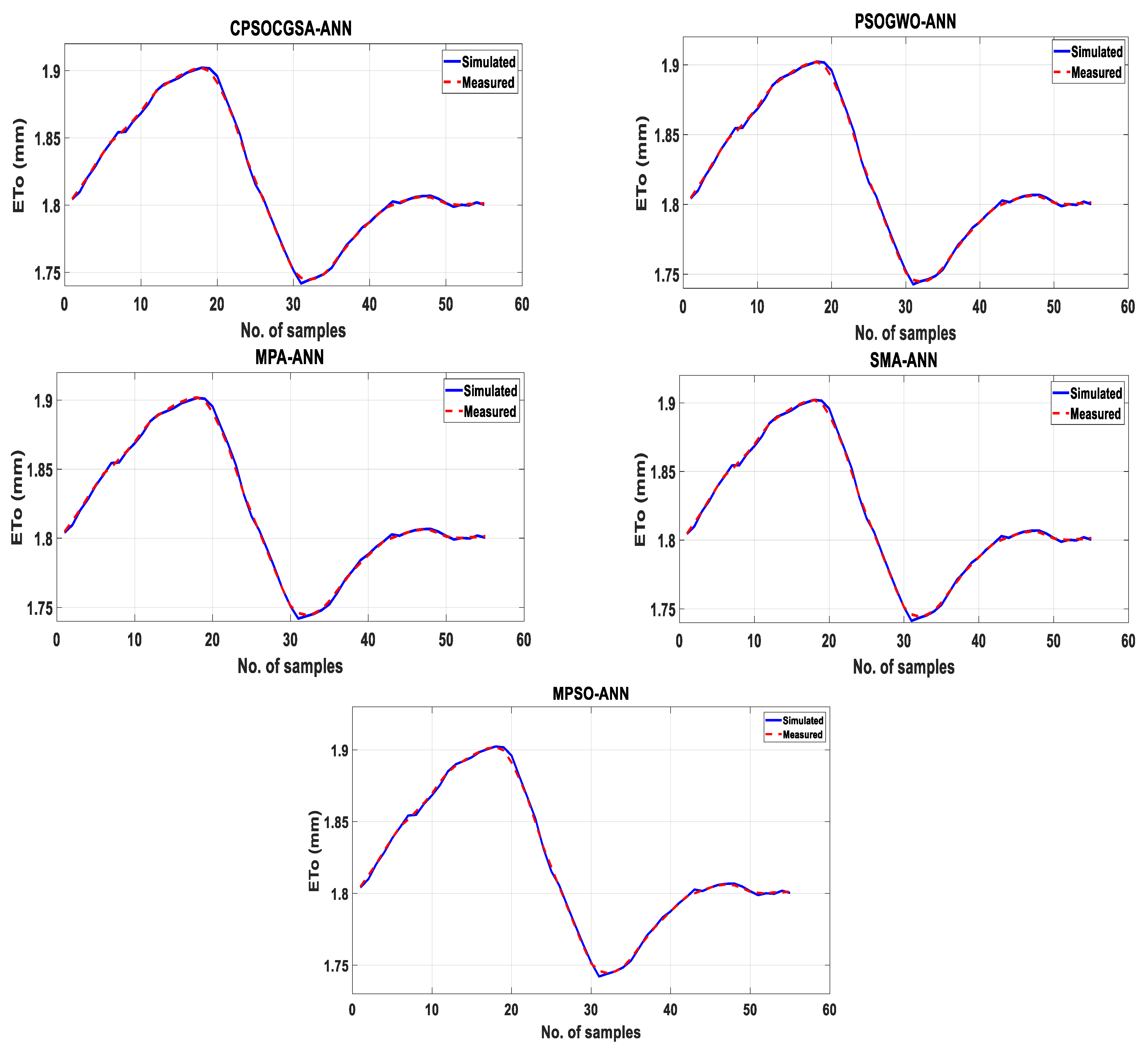
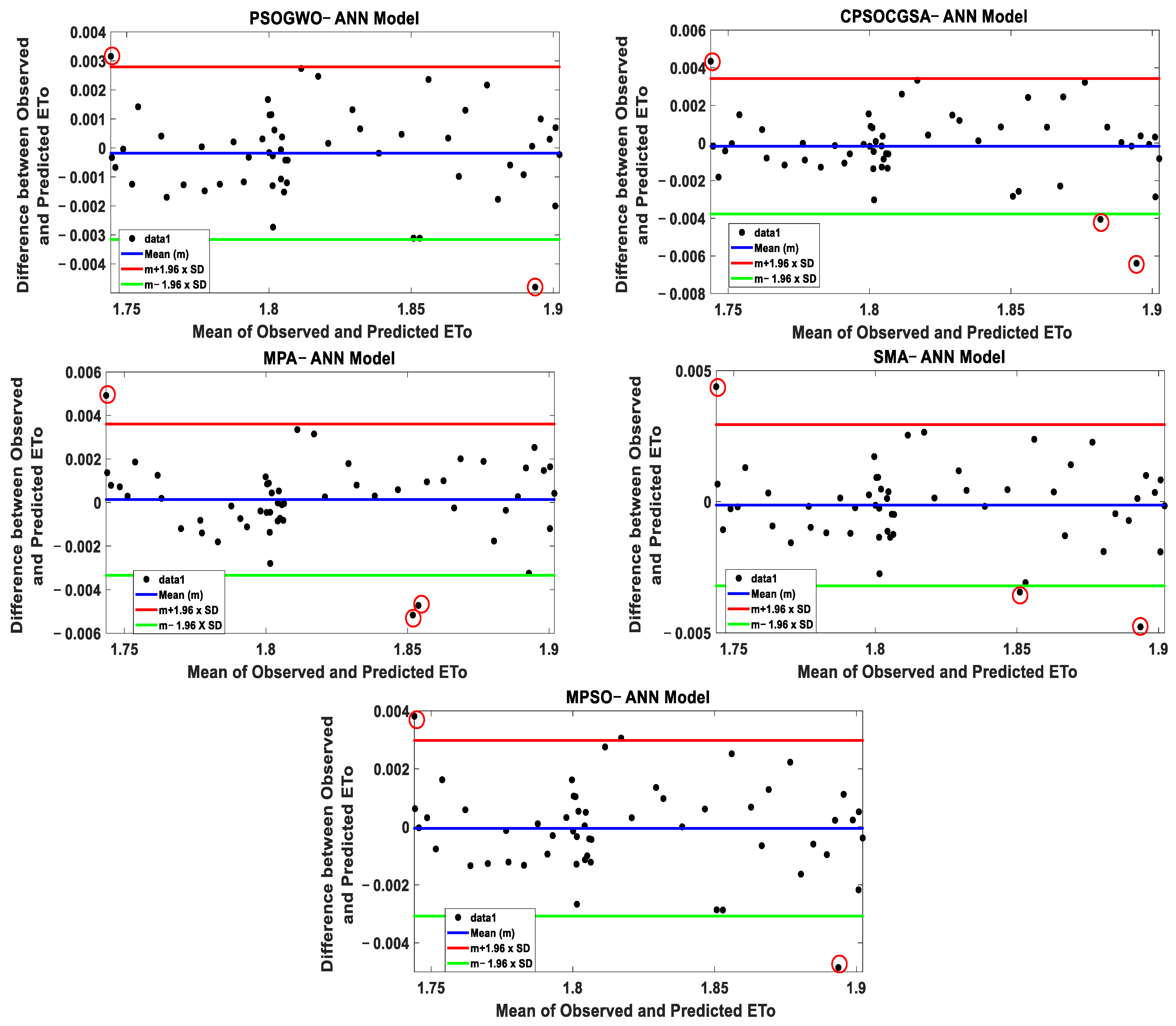
4.3. Performance Evaluation

After integrating the ANN technique by locating the optimal parameters, the model was run repeatedly (using MATLAB Neural Network Toolbox) to find the best network, weights and biases, to accurately predict the monthly ETo. A battery of statistical tests was conducted to determine whether or not ANN could generalise ETo data by considering four lags in the validation phase and to compare the effectiveness of the established strategies.

Table 3. Performance of the hybrid models for the validation data stage.

Model	RMSE	SI	NSE	R2
PSOGWO-ANN	0.00151	0.08317	0.99896	0.99899
CPSOCGSA-ANN	0.00153	0.0842	0.99893	0.99896
MPA-ANN	0.00159	0.08769	0.99884	0.99888
SMA-ANN	0.00154	0.08488	0.99892	0.99895
MPSO-ANN	0.00152	0.8396	0.99896	0.99894

displays the outcomes of four tests applied to assess the efficiency of the models. NSE and R² evaluate the linear dependence between measured and simulated ETo data, while RMSE and SI evaluate the nonlinear dependence. As stated in the Section 3.5, ANN models provide good to excellent accuracy. Nevertheless, ANN combined with the PSOGWO algorithm slightly outperforms the other models, which have the lowest RMSE and SI and the highest NSE and R².

Figure 8 presents the R² values for all the suggested hybrid models. The results of all models demonstrate good simulation levels for the ETo time series based on R², according to Dawson et al. [90]. R² values offer information about the linear relationship between the measured ETo value (i.e., computed by FAO56-PM, target) and predicted ETo value (output), for all models. The graphs demonstrate excellent levels of consistency between measured and forecast data, and the absence of any irregular data or distinct pattern trends.

Figure 9 compares the measured and simulated data for the validation phase from the PSOGWO-ANN, CPSOCGSA-ANN, MPA-ANN, SMA-ANN and MPSO-ANN models. The simulated data closely match the observed data pattern (trend + periodicity), along the time series.

The suggested hybrid techniques were further examined to verify the models’ power to accurately simulate monthly ETo in Al-Kut City. The Bland–Altman plot (Figure 10) is also taken into account to determine the degree of systematic variance, the scatter of values and whether there is a correlation between the observed and expected error. The results in Figure 10 are significant because the PSOGWO-ANN model has 96% of the data scattered between the red and green boundaries of the acceptable range, while the rest of the models contain 94% of the data scattered between the boundaries.

Regarding all the performance tests, the suggested techniques reveal good to excellent performance in simulating monthly ETo data in the validation phase. Nevertheless, ANN combined with the PSOGWO algorithm slightly outperformed the other models.

5. Discussion

Three pre-processing methods were applied in this research as the first stage of the suggested methodology: normalisation by natural logarithm, cleaning using the SSA technique and MI to select the best predictors. The first two pre-processing approaches enhance the quality of the raw data, whereby the CC of Lag 1 increased from 0.83 to 0.99. However, the most crucial step in developing any forecast strategy is identifying the number of predictors for the ML techniques. In this study, Figure 5 revealed that the first four lags were selected as the optimum model input by avoiding multicollinearity, which is vital for accurate ETo estimation. This is in line with the findings of Roy et al. [25] and Sayyahi et al. [15], which applied various variable selection techniques to determine the best number of predictors in order to produce the best possible forecast performance.

ML models have multiple disadvantages, such as a low rate of convergence and the difficulty of avoiding local minima. Recent advances in hybrid modelling have improved ML, paving the way for further development of standalone models to increase their accuracy [17]. A recent systematic review by Khairan et al. [17] analysed 33 previous studies on ETo data prediction using hybrid models. Thirty-three studies used ML models that integrated with a wide range of MHAs. All these studies, which apply to various areas and time scales, find that hybrid approaches perform better than standalone models.

Based on multiple statistical and graphical tests used to examine the models, as shown in Section 3.5, the results agree that both MHAs, i.e., single and hybrid algorithms, enhance the performance of the standalone ANN method when simulating ETo data. The hybrid MHAs slightly outperform single MHAs with R² of 0.99899, 0.99896, 0.99888, 0.99895 and 0.99894 for PSOGWO-ANN, CPSOCGSA-ANN, MPA-ANN, SMA-ANN and MPOS-ANN, respectively. PSOGWO-ANN is better at determining the optimal hyperparameters (Lr, N1 and N2) of the ANN technique and also saves time. These results reflect those of Adnan et al. [40] and Khalilpourazari and Khalilpourazary [91], who also found that hybrid MHAs outperform single MHAs. This finding may assist in better understanding and regulation of water balance processes. Further work could consider if the learning process can be improved by examining alternative tuning parameters for optimisers, and also applying training strategies, such as transfer learning and reinforcement learning.

6. Conclusions

This research offers a novel hybrid methodology to simulate monthly ETo data by combining an ANN model with the most contemporary PSOGWO algorithm and data preprocessing techniques. Monthly ETos have been forecast using a novel methodology, developed and tested using a number of prior lags. The performance of the PSOGWO method was evaluated and validated using the CPSOCGSA, MPA, SMA and MPSO-ANN algorithms; the following conclusions were drawn from this investigation in light of the findings:

• The data pre-processing procedures used in the present study, i.e., the use of SSA and MI, are essential for improving the quality of raw data and selecting the best lagged scenario, whereby the CC of Lag 1 increased from 0.83 to 0.99.
• ANN is an effective tool for predicting evapotranspiration. Integrating it with algorithms improves its performance and saves time by selecting the optimal Lr coefficient and N1 and N2 numbers.
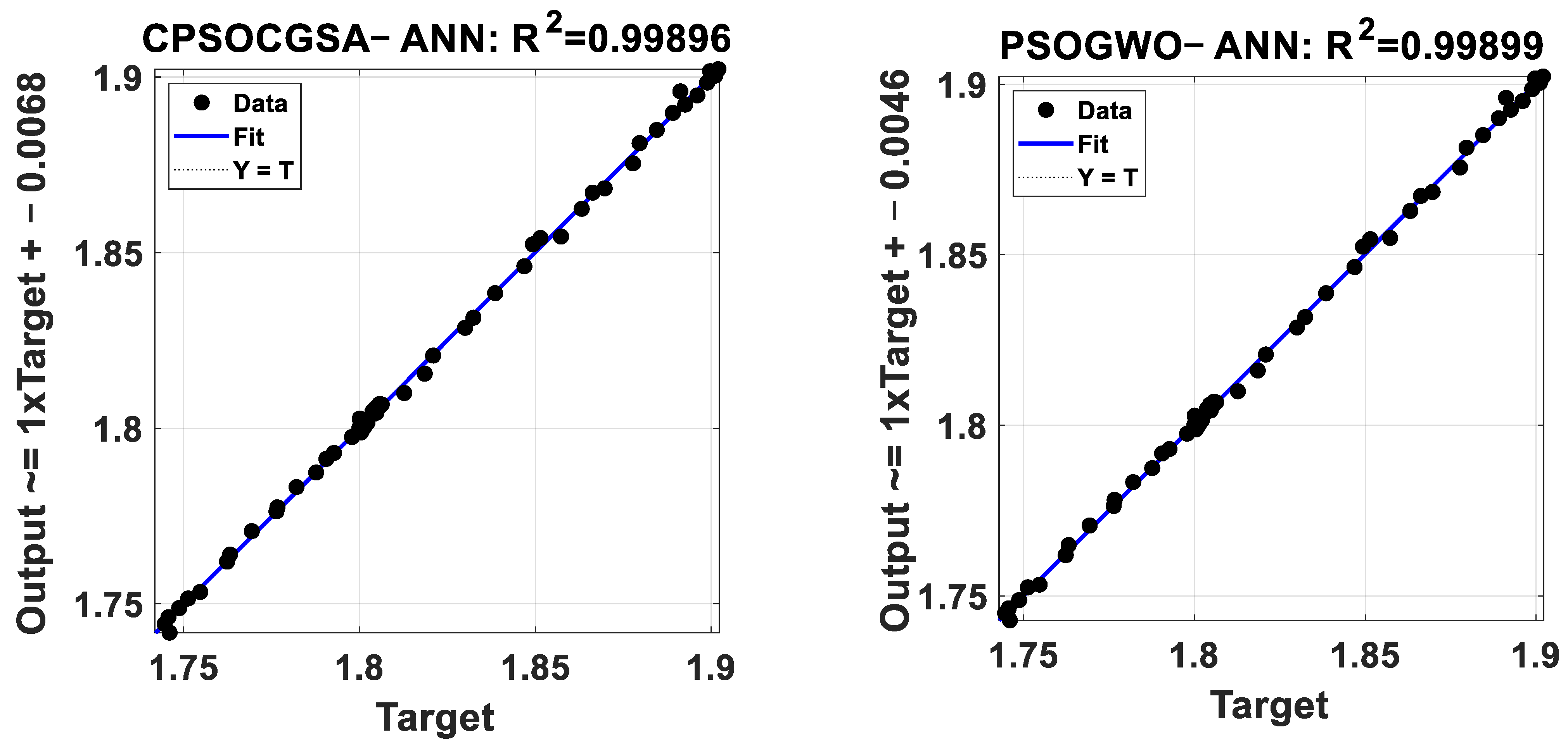
• All the forecasting models gave a good and similar performance, but it has been demonstrated that PSOGWO-ANN slightly outperformed other hybrid models. The best model shows that the suggested methodology is an accurate strategy for predicting monthly ETo, with R² = 0.99, RMSE = 0.00151, SI = 0.08317 and NSE = 0.99896.

Given the importance of wheat planting in Al-Kut City, this research may be useful in advising policymakers on how to allocate water supplies. Future research into the role of MHAs and data pre-processing approaches would be beneficial for researchers to improve HPOH strategies for ETo prediction models. The hybrid PSOGWO-ANN model is a promising technique for estimating monthly ETo in other agro-Iraqi provinces such as Kirkuk and Salahaddin and is therefore strongly recommended for this purpose.

References

1. Nourani, V.; Elkiran, G.; Abdullahi, J. Multi-step ahead modeling of reference evapotranspiration using a multi-model approach. J. Hydrol. 2020, 581, 124434. [Google Scholar] [CrossRef]
2. Hussain, M.I.; Muscolo, A.; Farooq, M.; Ahmad, W. Sustainable use and management of non-conventional water resources for rehabilitation of marginal lands in arid and semiarid environments. Agric. Water Manag. 2019, 221, 462–476. [Google Scholar] [CrossRef]
3. Raza, A.; Hu, Y.; Shoaib, M.; Abd Elnabi, M.K.; Zubair, M.; Nauman, M.; Syed, N.R. A systematic review on estimation of reference evapotranspiration under prisma guidelines. Pol. J. Environ. Stud 2021, 30, 5413–5422. [Google Scholar] [CrossRef]
4. Krishnashetty, P.H.; Balasangameshwara, J.; Sreeman, S.; Desai, S.; Kantharaju, A.B. Cognitive computing models for estimation of reference evapotranspiration: A review. Cogn. Syst. Res. 2021, 70, 109–116. [Google Scholar] [CrossRef]
5. Roy, D.K. Long Short-Term Memory Networks to Predict One-Step Ahead Reference Evapotranspiration in a Subtropical Climatic Zone. Environ. Process. 2021, 8, 911–941. [Google Scholar] [CrossRef]
6. Sabziparvar, A.A.; Mirmasoudi, S.H.; Tabari, H.; Nazemosadat, M.J.; Maryanaji, Z. ENSO teleconnection impacts on reference evapotranspiration variability in some warm climates of Iran. Int. J. Climatol. 2011, 31, 1710–1723. [Google Scholar] [CrossRef]
7. Proias, G.; Gravalos, I.; Papageorgiou, E.; Poczęta, K.; Sakellariou-Makrantonaki, M. Forecasting Reference Evapotranspiration Using Time Lagged Recurrent Neural Network. Wseas Trans. Environ. Dev. 2020, 16, 699–707. [Google Scholar] [CrossRef]
8. Muhammad Adnan, R.; Chen, Z.; Yuan, X.; Kisi, O.; El-Shafie, A.; Kuriqi, A.; Ikram, M. Reference Evapotranspiration Modeling Using New Heuristic Methods. Entropy 2020, 22, 547. [Google Scholar] [CrossRef]
9. Alawsi, M.A.; Zubaidi, S.L.; Al-Ansari, N.; Al-Bugharbee, H.; Ridha, H.M. Tuning ANN Hyperparameters by CPSOCGSA, MPA, and SMA for Short-Term SPI Drought Forecasting. Atmosphere 2022, 13, 1436. [Google Scholar] [CrossRef]
10. Ethaib, S.; Zubaidi, S.L.; Al-Ansari, N. Evaluation water scarcity based on GIS estimation and climate-change effects: A case study of Thi-Qar Governorate, Iraq. Cogent Eng. 2022, 9, 2075301. [Google Scholar] [CrossRef]
11. IOM. Migration, Environment, and Climate Change in Iraq; International Organization for Migration (IOM): Baghdad, Iraq, 2022; pp. 1–32. [Google Scholar]
12. Ferreira, L.B.; da Cunha, F.F. Multi-step ahead forecasting of daily reference evapotranspiration using deep learning. Comput. Electron. Agric. 2020, 178, 105728. [Google Scholar] [CrossRef]
13. Roy, D.K.; Barzegar, R.; Quilty, J.; Adamowski, J. Using ensembles of adaptive neuro-fuzzy inference system and optimization algorithms to predict reference evapotranspiration in subtropical climatic zones. J. Hydrol. 2020, 591, 125509. [Google Scholar] [CrossRef]
14. Naganna, S.R.; Beyaztas, B.H.; Bokde, N.; Armanuos, A.M. On the evaluation of the gradient tree boosting model for groundwater level forecasting. Knowl.-Based Eng. 2020, 1, 48–57. [Google Scholar] [CrossRef]
15. Sayyahi, F.; Farzin, S.; Karami, H.; Cai, N. Forecasting Daily and Monthly Reference Evapotranspiration in the Aidoghmoush Basin Using Multilayer Perceptron Coupled with Water Wave Optimization. Complexity 2021, 2021, 6683759. [Google Scholar] [CrossRef]
16. Yaghoubzadeh-Bavandpour, A.; Bozorg-Haddad, O.; Rajabi, M.; Zolghadr-Asli, B.; Chu, X. Application of swarm intelligence and evolutionary computation algorithms for optimal reservoir operation. Water Resour. Manag. 2022, 36, 2275–2292. [Google Scholar] [CrossRef]
17. Khairan, H.E.; Zubaidi, S.L.; Muhsen, Y.R.; Al-Ansari, N. Parameter Optimisation Based Hybrid Reference Evapotranspiration Prediction Models A Systematic Review of Current Implementations and Future Research Directions. Atmosphere 2022, 14, 77. [Google Scholar] [CrossRef]
18. Khudhair, Z.S.; Zubaidi, S.L.; Ortega-Martorell, S.; Al-Ansari, N.; Ethaib, S.; Hashim, K.J.E. A Review of Hybrid Soft Computing and Data Pre-Processing Techniques to Forecast Freshwater Quality’s Parameters: Current Trends and Future Directions. Environments 2022, 9, 85. [Google Scholar] [CrossRef]
19. Mohammed, S.J.; Zubaidi, S.L.; Ortega-Martorell, S.; Al-Ansari, N.; Ethaib, S.; Hashim, K.J.C.E. Application of hybrid machine learning models and data pre-processing to predict water level of watersheds: Recent trends and future perspective. Cogent Eng. 2022, 9, 2143051. [Google Scholar] [CrossRef]
20. Merchaoui, M.; Sakly, A.; Mimouni, M.F. Particle swarm optimisation with adaptive mutation strategy for photovoltaic solar cell/module parameter extraction. Energy Convers. Manag. 2018, 175, 151–163. [Google Scholar] [CrossRef]
21. Chen, H.; Jiao, S.; Wang, M.; Heidari, A.A.; Zhao, X. Parameters identification of photovoltaic cells and modules using diversification-enriched Harris hawks optimization with chaotic drifts. J. Clean. Prod. 2020, 244, 118778. [Google Scholar] [CrossRef]
22. Ridha, H.M. Parameters extraction of single and double diodes photovoltaic models using Marine Predators Algorithm and Lambert W function. Sol. Energy 2020, 209, 674–693. [Google Scholar] [CrossRef]
23. Wolpert, D.H.; Macready, W.G. No free lunch theorems for optimization. IEEE Trans. Evol. Comput. 1997, 1, 67–82. [Google Scholar] [CrossRef]
24. Adetunji, K.E.; Hofsajer, I.W.; Abu-Mahfouz, A.M.; Cheng, L. A Review of Metaheuristic Techniques for Optimal Integration of Electrical Units in Distribution Networks. IEEE Access 2021, 9, 5046–5068. [Google Scholar] [CrossRef]
25. Roy, D.K.; Lal, A.; Sarker, K.K.; Saha, K.K.; Datta, B. Optimization algorithms as training approaches for prediction of reference evapotranspiration using adaptive neuro fuzzy inference system. Agric. Water Manag. 2021, 255, 107003. [Google Scholar] [CrossRef]
26. Almubaidin, M.A.A.; Ahmed, A.N.; Sidek, L.B.M.; Elshafie, A. Using Metaheuristics Algorithms (MHAs) to Optimize Water Supply Operation in Reservoirs: A Review. Arch. Comput. Methods Eng. 2022, 29, 3677–3711. [Google Scholar] [CrossRef]
27. Lai, V.; Essam, Y.; Huang, Y.F.; Ahmed, A.N.; El-Shafie, A. Investigating dam reservoir operation optimization using metaheuristic algorithms. Appl. Water Sci. 2022, 12, 280. [Google Scholar] [CrossRef]
28. Li, S.; Chen, H.; Wang, M.; Heidari, A.A.; Mirjalili, S. Slime mould algorithm: A new method for stochastic optimization. Future Gener. Comput. Syst. 2020, 111, 300–323. [Google Scholar] [CrossRef]
29. ElSayed, S.K.; Elattar, E.E. Slime mold algorithm for optimal reactive power dispatch combining with renewable energy sources. Sustainability 2021, 13, 5831. [Google Scholar] [CrossRef]
30. Houssein, E.H.; Mahdy, M.A.; Blondin, M.J.; Shebl, D.; Mohamed, W.M. Hybrid slime mould algorithm with adaptive guided differential evolution algorithm for combinatorial and global optimization problems. Expert Syst. Appl. 2021, 174, 114689. [Google Scholar] [CrossRef]
31. Kumar, C.; Raj, T.D.; Premkumar, M.; Raj, T.D. A new stochastic slime mould optimization algorithm for the estimation of solar photovoltaic cell parameters. Optik 2020, 223, 165277. [Google Scholar] [CrossRef]
32. Faramarzi, A.; Heidarinejad, M.; Mirjalili, S.; Gandomi, A.H. Marine Predators Algorithm: A nature-inspired metaheuristic. Expert Syst. Appl. 2020, 152, 113377. [Google Scholar] [CrossRef]
33. Ghafil, H.N.; Jármai, K. Dynamic differential annealed optimization: New metaheuristic optimization algorithm for engineering applications. Appl. Soft Comput. 2020, 93, 106392. [Google Scholar] [CrossRef]
34. Eid, A.; Kamel, S.; Abualigah, L. Marine predators algorithm for optimal allocation of active and reactive power resources in distribution networks. Neural Comput. Appl. 2021, 33, 14327–14355. [Google Scholar] [CrossRef]
35. Rather, S.A.; Bala, P.S. A hybrid constriction coefficient-based particle swarm optimization and gravitational search algorithm for training multi-layer perceptron. Int. J. Intell. Comput. Cybern. 2020, 13, 129–165. [Google Scholar] [CrossRef]
36. Ahmadi, F.; Mehdizadeh, S.; Mohammadi, B.; Pham, Q.B.; Doan, T.N.C.; Vo, N.D. Application of an artificial intelligence technique enhanced with intelligent water drops for monthly reference evapotranspiration estimation. Agric. Water Manag. 2021, 244, 106622. [Google Scholar] [CrossRef]
37. Tao, H.; Diop, L.; Bodian, A.; Djaman, K.; Ndiaye, P.M.; Yaseen, Z.M. Reference evapotranspiration prediction using hybridized fuzzy model with firefly algorithm: Regional case study in Burkina Faso. Agric. Water Manag. 2018, 208, 140–151. [Google Scholar] [CrossRef]
38. Maroufpoor, S.; Bozorg-Haddad, O.; Maroufpoor, E. Reference evapotranspiration estimating based on optimal input combination and hybrid artificial intelligent model: Hybridization of artificial neural network with grey wolf optimizer algorithm. J. Hydrol. 2020, 588, 125060. [Google Scholar] [CrossRef]
39. Chica, M.; Juan Pérez, A.A.; Cordon, O.; Kelton, D. Why simheuristics? Benefits, limitations, and best practices when combining metaheuristics with simulation. SORT 2017, 44, 311–334. [Google Scholar] [CrossRef]
40. Adnan, R.M.; Mostafa, R.R.; Islam, A.R.M.T.; Kisi, O.; Kuriqi, A.; Heddam, S. Estimating reference evapotranspiration using hybrid adaptive fuzzy inferencing coupled with heuristic algorithms. Comput. Electron. Agric. 2021, 191, 106541. [Google Scholar] [CrossRef]
41. Rather, S.A.; Bala, P.S. Hybridization of constriction coefficient-based particle swarm optimization and chaotic gravitational search algorithm for solving engineering design problems. Appl. Soft Comput. Commun. Netw. Proc. ACN 2020, 125, 95–115. [Google Scholar]
42. Črepinšek, M.; Liu, S.-H.; Mernik, M. Exploration and exploitation in evolutionary algorithms: A survey. ACM Comput. Surv. 2013, 45, 1–33. [Google Scholar] [CrossRef]
43. Eiben, A.E.; Schippers, C.A. On evolutionary exploration and exploitation. Fundam. Informaticae 1998, 35, 35–50. [Google Scholar] [CrossRef]
44. Şenel, F.A.; Gökçe, F.; Yüksel, A.S.; Yiğit, T. A novel hybrid PSO–GWO algorithm for optimization problems. Eng. Comput. 2019, 35, 1359–1373. [Google Scholar] [CrossRef]
45. Hajirahimi, Z.; Khashei, M. Hybridization of hybrid structures for time series forecasting: A review. Artif. Intell. Rev. 2022, 56, 1201–1261. [Google Scholar] [CrossRef]
46. Zubaidi, S.L.; Al-Bdairi, N.S.S.; Ortega-Martorell, S.; Ridha, H.M.; Al-Ansari, N.; Al-Bugharbee, H.; Hashim, K.; Gharghan, S.K. Assessing the Benefits of Nature-Inspired Algorithms for the Parameterization of ANN in the Prediction of Water Demand. J. Water Resour. Plan. Manag. 2023, 149, 1–10. [Google Scholar] [CrossRef]
47. Edan, M.H.; Maarouf, R.M.; Hasson, J. Predicting the impacts of land use/land cover change on land surface temperature using remote sensing approach in Al Kut, Iraq. Phys. Chem. Earth Parts A/B/C 2021, 123, 103012. [Google Scholar] [CrossRef]
48. Muter, S.A.; Nassif, W.G.; Al-Ramahy, Z.A.; Al-Taai, O.T. Analysis of seasonal and annual relative humidity using GIS for selected stations over Iraq during the period (1980–2017). J. Green Eng. 2020, 10, 9121–9135. [Google Scholar]
49. Al-Abadi, A.; Al-Aboodi, A.H.D. Optimum rain-gauges network design of some cities in Iraq. J. Babylon Univ./Eng. Sci. 2014, 22, 946–958. [Google Scholar]
50. Capt, T.; Mirchi, A.; Kumar, S.; Walker, W.S. Urban Water Demand: Statistical Optimization Approach to Modeling Daily Demand. J. Water Resour. Plan. Manag. 2021, 147, 1–10. [Google Scholar] [CrossRef]
51. Allen, R.G.; Pereira, L.S.; Raes, D.; Smith, M. Crop Evapotranspiration-Guidelines for Computing Crop Water Requirements-FAO Irrigation and Drainage Paper 56; FAO: Rome, Italy, 1998; Volume 300, p. D05109. [Google Scholar]
52. Yu, J.; Zheng, W.; Xu, L.; Zhangzhong, L.; Zhang, G.; Shan, F. A PSO-XGBoost Model for Estimating Daily Reference Evapotranspiration in the Solar Greenhouse. Intell. Autom. Soft Comput. 2020, 26, 989–1003. [Google Scholar] [CrossRef]
53. Behboudian, S.; Tabesh, M.; Falahnezhad, M.; Ghavanini, F.A. A long-term prediction of domestic water demand using preprocessing in artificial neural network. J. Water Supply Res. Technol.-Aqua 2014, 63, 31–42. [Google Scholar] [CrossRef]
54. Espinosa, F.; Bartolomé, A.B.; Hernández, P.V.; Rodriguez-Sanchez, M. Contribution of Singular Spectral Analysis to Forecasting and Anomalies Detection of Indoors Air Quality. Sensors 2022, 22, 3054. [Google Scholar] [CrossRef] [PubMed]
55. Al-Bugharbee, H.; Trendafilova, I. A fault diagnosis methodology for rolling element bearings based on advanced signal pretreatment and autoregressive modelling. J. Sound Vib. 2016, 369, 246–265. [Google Scholar] [CrossRef]
56. Bureneva, O.; Safyannikov, N.; Aleksanyan, Z. Singular Spectrum Analysis of Tremorograms for Human Neuromotor Reaction Estimation. Mathematics 2022, 10, 1794. [Google Scholar] [CrossRef]
57. Kilundu, B.; Chiementin, X.; Dehombreux, P. Singular spectrum analysis for bearing defect detection. J. Vib. Acoust. 2011, 133, 051007. [Google Scholar] [CrossRef]
58. Hassani, H. Singular spectrum analysis: Methodology and comparison. J. Data Sci. 2007, 5, 239–257. [Google Scholar] [CrossRef] [PubMed]
59. Pham, Q.B.; Yang, T.-C.; Kuo, C.-M.; Tseng, H.-W.; Yu, P.-S. Coupling singular spectrum analysis with least square support vector machine to improve accuracy of SPI drought forecasting. Water Resour. Manag. 2021, 35, 847–868. [Google Scholar] [CrossRef]
60. Ouyang, Q.; Lu, W. Monthly rainfall forecasting using echo state networks coupled with data preprocessing methods. Water Resour. Manag. 2018, 32, 659–674. [Google Scholar] [CrossRef]
61. Apaydin, H.; Sattari, M.T.; Falsafian, K.; Prasad, R. Artificial intelligence modelling integrated with Singular Spectral analysis and Seasonal-Trend decomposition using Loess approaches for streamflow predictions. J. Hydrol. 2021, 600, 126506. [Google Scholar] [CrossRef]
62. Danandeh Mehr, A.; Ghadimi, S.; Marttila, H.; Torabi Haghighi, A.; Climatology, A. A new evolutionary time series model for streamflow forecasting in boreal lake-river systems. Theor. Appl. Climatol. 2022, 148, 255–268. [Google Scholar] [CrossRef]
63. Ramírez-Rojas, A.; Cárdenas-Moreno, P.; Vargas, C. Mutual information analysis between NO2 and O3 pollutants measured in Mexico City before and during 2020 COVID-19 pandemic year. J. Phys. Conf. Ser. 2022, 2307, 012053. [Google Scholar] [CrossRef]
64. Mirjalili, S.; Mirjalili, S.M.; Lewis, A. Grey wolf optimizer. Adv. Eng. Softw. 2014, 69, 46–61. [Google Scholar] [CrossRef]
65. Dong, J.; Liu, X.; Huang, G.; Fan, J.; Wu, L.; Wu, J. Comparison of four bio-inspired algorithms to optimize KNEA for predicting monthly reference evapotranspiration in different climate zones of China. Comput. Electron. Agric. 2021, 186, 106211. [Google Scholar] [CrossRef]
66. Kennedy, J.; Eberhart, R. Particle swarm optimization. In Proceedings of the ICNN’95-International Conference on Neural Networks, Perth, Australia, 27 November–1 December 1995; pp. 1942–1948. [Google Scholar]
67. Zhu, B.; Feng, Y.; Gong, D.; Jiang, S.; Zhao, L.; Cui, N. Hybrid particle swarm optimization with extreme learning machine for daily reference evapotranspiration prediction from limited climatic data. Comput. Electron. Agric. 2020, 173, 105430. [Google Scholar] [CrossRef]
68. Roy, D.K.; Saha, K.K.; Kamruzzaman, M.; Biswas, S.K.; Hossain, M.A. Hierarchical Fuzzy Systems Integrated with Particle Swarm Optimization for Daily Reference Evapotranspiration Prediction: A Novel Approach. Water Resour. Manag. 2021, 35, 5383–5407. [Google Scholar] [CrossRef]
69. Alizamir, M.; Kisi, O.; Muhammad Adnan, R.; Kuriqi, A. Modelling reference evapotranspiration by combining neuro-fuzzy and evolutionary strategies. Acta Geophys. 2020, 68, 1113–1126. [Google Scholar] [CrossRef]
70. Jawad, H.M.; Jawad, A.M.; Nordin, R.; Gharghan, S.K.; Abdullah, N.F.; Ismail, M.; Abu-AlShaeer, M.J. Accurate empirical path-loss model based on particle swarm optimization for wireless sensor networks in smart agriculture. IEEE Sens. J. 2019, 20, 552–561. [Google Scholar] [CrossRef]
71. Peng, T.; Zhou, J.; Zhang, C.; Fu, W. Streamflow forecasting using empirical wavelet transform and artificial neural networks. Water 2017, 9, 406. [Google Scholar] [CrossRef]
72. Nabipour, N.; Dehghani, M.; Mosavi, A.; Shamshirband, S. Short-term hydrological drought forecasting based on different nature-inspired optimization algorithms hybridized with artificial neural networks. IEEE Access 2020, 8, 15210–15222. [Google Scholar] [CrossRef]
73. Tikhamarine, Y.; Malik, A.; Kumar, A.; Souag-Gamane, D.; Kisi, O. Estimation of monthly reference evapotranspiration using novel hybrid machine learning approaches. Hydrol. Sci. J. 2019, 64, 1824–1842. [Google Scholar] [CrossRef]
74. Zhang, N.; Hwang, B.-G.; Lu, Y.; Ngo, J. A Behavior theory integrated ANN analytical approach for understanding households adoption decisions of residential photovoltaic (RPV) system. Technol. Soc. 2022, 70, 102062. [Google Scholar] [CrossRef]
75. Gocić, M.; Arab Amiri, M. Reference Evapotranspiration Prediction Using Neural Networks and Optimum Time Lags. Water Resour. Manag. 2021, 35, 1913–1926. [Google Scholar] [CrossRef]
76. Pourdarbani, R.; Sabzi, S.; Rohban, M.H.; Garcia-Mateos, G.; Paliwal, J.; Molina-Martinez, J.M. Using metaheuristic algorithms to improve the estimation of acidity in Fuji apples using NIR spectroscopy. Ain Shams Eng. J. 2022, 13, 101776. [Google Scholar] [CrossRef]
77. Kapanova, K.G.; Dimov, I.; Sellier, J.M. A genetic approach to automatic neural network architecture optimization. Neural Comput. Appl. 2016, 29, 1481–1492. [Google Scholar] [CrossRef]
78. Alemu, H.; Wu, W.; Zhao, J. Feedforward Neural Networks with a Hidden Layer Regularization Method. Symmetry 2018, 10, 525. [Google Scholar] [CrossRef]
79. Yahya-Khotbehsara, A.; Shahhoseini, A. A fast modeling of the double-diode model for PV modules using combined analytical and numerical approach. Sol. Energy 2018, 162, 403–409. [Google Scholar] [CrossRef]
80. Ahmed, A.N.; Van Lam, T.; Hung, N.D.; Van Thieu, N.; Kisi, O.; El-Shafie, A. A comprehensive comparison of recent developed meta-heuristic algorithms for streamflow time series forecasting problem. Appl. Soft Comput. 2021, 105, 107282. [Google Scholar] [CrossRef]
81. Legates, D.R.; McCabe Jr, G.J. Evaluating the use of “goodness-of-fit” measures in hydrologic and hydroclimatic model validation. Water Resour. Res. 1999, 35, 233–241. [Google Scholar] [CrossRef]
82. Hodges, G.; Eadsforth, C.; Bossuyt, B.; Bouvy, A.; Enrici, M.-H.; Geurts, M.; Kotthoff, M.; Michie, E.; Miller, D.; Müller, J.; et al. A comparison of log Kow (n-octanol–water partition coefficient) values for non-ionic, anionic, cationic and amphoteric surfactants determined using predictions and experimental methods. Environ. Sci. Eur. 2019, 31, 1. [Google Scholar] [CrossRef]
83. Shiri, J.; Zounemat-Kermani, M.; Kisi, O.; Mohsenzadeh Karimi, S. Comprehensive assessment of 12 soft computing approaches for modelling reference evapotranspiration in humid locations. Meteorol. Appl. 2019, 27, e1841. [Google Scholar] [CrossRef]
84. Wang, W.; Kong, W.; Shen, T.; Man, Z.; Zhu, W.; He, Y.; Liu, F. Quantitative analysis of cadmium in rice roots based on LIBS and chemometrics methods. Environ. Sci. Eur. 2021, 33, 37. [Google Scholar] [CrossRef]
85. Despotovic, M.; Nedic, V.; Despotovic, D.; Cvetanovic, S. Review and statistical analysis of different global solar radiation sunshine models. Renew. Sustain. Energy Rev. 2015, 52, 1869–1880. [Google Scholar] [CrossRef]
86. Jain, S.K.; Sudheer, K. Fitting of hydrologic models: A close look at the Nash–Sutcliffe index. J. Hydrol. Eng. 2008, 13, 981–986. [Google Scholar] [CrossRef]
87. Pan, M.; Zhou, H.; Cao, J.; Liu, Y.; Hao, J.; Li, S.; Chen, C.-H. Water level prediction model based on GRU and CNN. IEEE Access 2020, 8, 60090–60100. [Google Scholar] [CrossRef]
88. Stergiou, N. Nonlinear Analysis for Human Movement Variability; CRC Press: Boca Raton, FL, USA, 2018. [Google Scholar]
89. Tabachnick, B.G.; Fidell, L.S.; Ullman, J.B. Using Multivariate Statistics; Pearson: Boston, MA, USA, 2013; Volume 6. [Google Scholar]
90. Dawson, C.W.; Abrahart, R.J.; See, L.M. HydroTest: A web-based toolbox of evaluation metrics for the standardised assessment of hydrological forecasts. Environ. Model. Softw. 2007, 22, 1034–1052. [Google Scholar] [CrossRef]
91. Khalilpourazari, S.; Khalilpourazary, S. An efficient hybrid algorithm based on Water Cycle and Moth-Flame Optimization algorithms for solving numerical and constrained engineering optimization problems. Soft Comput. 2019, 23, 1699–1722. [Google Scholar] [CrossRef]
Figure 1. A map showing the location of the research site (Wasit Province).
Sustainability 15 14222 g001
Figure 2. A workflow diagram showing the steps involved in univariate ETo simulation.
Sustainability 15 14222 g002
Figure 3. PSOGWO algorithm flowchart.
Sustainability 15 14222 g003
Figure 4. Normalised data and the first four components were acquired using SSA.
Sustainability 15 14222 g004
Figure 5. Average mutual information (AMI) as a function of the ETo time series.
Sustainability 15 14222 g005
Figure 6. Performance of the PSOGWO algorithm.
Sustainability 15 14222 g006
Figure 7. Fitness function of suggested hybrid algorithms under five popsizes.
Sustainability 15 14222 g007
Figure 8. Coefficients of determination for the suggested models.
Sustainability 15 14222 g008aSustainability 15 14222 g008b
Figure 9. Measured and simulated ETo data comparison for all suggested strategies in the validation phase.
Sustainability 15 14222 g009
Figure 10. Bland–Altman plot of the suggested hybrid techniques in the validation stage.
Sustainability 15 14222 g010