
A Two-Stage Real-Time Optimization Model of Arterial Signal Coordination Based on Reverse Causal-Effect Modeling Approach


Abstract
:1. Introduction
2. Model Formulation
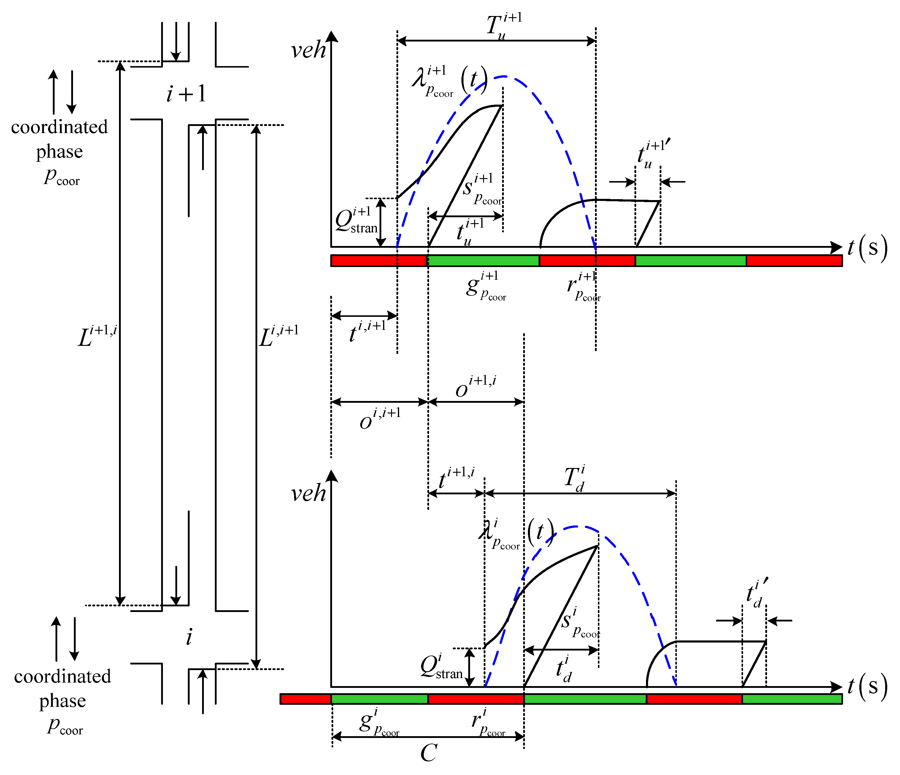
2.1. Offset Model for Two-Way Arterial Signal Coordination
- (1)
- Delay before and during the green time
- (2)
- Delay during the red time
- (3)
- Delay of the coordinated direction under the two-way arterial signal coordination
2.2. Two-Way Arterial Signal Coordination Model Based on Reverse Causal-Effect Modeling Approach
2.2.1. Intersection Signal Timing Model Based on Reverse Causal-Effect Modeling Approach
2.2.2. Offset Real-Time Optimization Model Based on Reverse Causal-Effect Modeling Approach
2.3. Model Solving
2.3.1. Model Simplification
- (1)
- The first stage model (M.2) simplification
- (2)
- The second stage model (M.1) simplification
2.3.2. Solution Algorithm
3. Case Study
4. Conclusions
Author Contributions
Funding
Institutional Review Board Statement
Informed Consent Statement
Data Availability Statement
Conflicts of Interest
Appendix A

References
- Little, J.D. The synchronization of traffic signals by mixed-integer linear programming. Oper. Res. 1966, 14, 568–594. [Google Scholar] [CrossRef]
- Gartner, N.H.; Stamatiadis, C. Arterial-based control of traffic flow in urban grid networks. Math. Comput. Model. 2002, 35, 657–671. [Google Scholar] [CrossRef]
- Zhang, C.; Xie, Y.; Gartner, N.H.; Stamatiadis, C.; Arsava, T. AM-band: An asymmetrical multi-band model for arterial traffic signal coordination. Transp. Res. Part C Emerg. Technol. 2015, 58, 515–531. [Google Scholar] [CrossRef]
- Yu, D.X.; Tian, X.J.; Yang, Z.S.; Zhou, X.Y.; Cheng, Z.Y. Improved arterial coordinated signal control optimization model. J. Zhejiang Univ. Eng. Sci. 2017, 51, 2019–2029. [Google Scholar]
- Zhang, Y.Y.; Li, J.L.; Zhang, Y.B. Study on green wave coordination control method based on ripple changes. J. Transp. Eng. Inf. 2019, 17, 52–61. [Google Scholar]
- Yu, J.J.; Ji, Y.J.; Bu, Q.; Zheng, Y.B. Partitioned green-wave control scheme for long arterial considering breakpoint cost. J. Zhejiang Univ. Eng. Sci. 2022, 4, 640–648. [Google Scholar]
- Clayton, A.J.H. Road traffic calculations. J. Inst. Civ. Eng. 1941, 16, 247–264. [Google Scholar] [CrossRef]
- Webster, F.V. Traffic Signal Settings; Road Research Technical Paper No. 39; Department of Scientific and Industrial Research: London, UK, 1958.
- Hillier, J.A.; Rothery, R. The synchronization of traffic signals for minimum delay. Transp. Sci. 1967, 1, 81–94. [Google Scholar] [CrossRef]
- Lieberman, E.B.; Woo, J.L. SIGOP II: A new computer program for calculating optimal signal timing patterns. Transp. Res. Rec. 1976, 596, 16–21. [Google Scholar]
- Benekohal, R.F.; El-Zohairy, Y.M. Multi-regime arrival rate uniform delay models for signalized intersections. Transp. Res. Part A Policy Pract. 2001, 35, 625–667. [Google Scholar] [CrossRef]
- Shenoda, M. Development of a Phase-by-Phase, Arrival-Based, Delay-Optimized Adaptive Traffic Signal Control Methodology with Metaheuristic Searc; The University of Texas: Austin, TX, USA, 2006. [Google Scholar]
- Ma, W.; An, K.; Lo, H.K. Multi-stage stochastic program to optimize signal timings under coordinated adaptive control. Transp. Res. Part C Emerg. Technol. 2016, 72, 342–359. [Google Scholar] [CrossRef]
- Wang, H.; Peng, X.Y. Coordinated control model for oversaturated arterial intersections. IEEE Trans. Intell. Transp. Syst. 2022, 23, 24157–24175. [Google Scholar] [CrossRef]
- Lee, S.; Messer, C.J. Evaluation of actuated control of diamond interchanges with advanced experimental design. J. Adv. Transp. 2003, 37, 195–210. [Google Scholar] [CrossRef]
- Zheng, X.; Recker, W. An adaptive control algorithm for traffic-actuated signals. Transp. Res. Part C Emerg. Technol. 2013, 30, 93–115. [Google Scholar] [CrossRef]
- Yin, Y.; Li, M.; Skabardonis, A. Offline offset refiner for coordinated actuated signal control systems. J. Transp. Eng. 2007, 133, 423–432. [Google Scholar] [CrossRef]
- Zhang, L.; Lou, Y. Coordination of semi-actuated signals on arterials. J. Adv. Transp. 2015, 49, 228–246. [Google Scholar] [CrossRef]
- Cesme, B.; Furth, P.G. Self-organizing traffic signals using secondary extension and dynamic coordination. Transp. Res. Part C Emerg. Technol. 2014, 48, 1–15. [Google Scholar] [CrossRef]
- He, Q.; Head, K.L.; Ding, J. Multi-modal traffic signal control with priority, signal actuation and coordination. Transp. Res. Part C Emerg. Technol. 2014, 46, 65–82. [Google Scholar] [CrossRef]
- Zhai, R. Analysis on Principle of Traffic Signal Coordinated Control for Arterial Road; Chinese people’s Public Security University Press: Beijing, China, 2020; pp. 313–355. [Google Scholar]
- Liu, H.; Balke, K.N.; Lin, W.H. A reverse causal-effect modeling approach for signal control of an oversaturated intersection. Transp. Res. Part C Emerg. Technol. 2008, 16, 742–754. [Google Scholar] [CrossRef]
- Lo, H.K. A reliability framework for traffic signal control. IEEE Trans. Intell. Transp. Syst. 2006, 7, 250–260. [Google Scholar] [CrossRef]


| The set of intersection, indexed by i | |
| The number of cycles | |
| The green time of intersection i in phase p (s) | |
| The red time of intersection i in phase p (s) | |
| The offset between the adjacent intersection i and i + 1(s) | |
| The green time ratio in phase p of intersection i | |
| The set of signal phases, indexed by p | |
| The length of a signal cycle (s) | |
| The set of allowable traffic streams in phase p, indexed by m | |
| The arrival rate for traffic stream m in phase p of intersection i (veh/h) | |
| The average saturation outflow rate of intersection i in phase p (veh/h) | |
| The outflow rate for traffic stream m in phase p of intersection i (veh/h) | |
| The average speed of vehicles from intersection i to intersection i + 1 (m/s) | |
| The distance from intersection i to intersection i + 1 (m) | |
| The time difference between the time at the start of green at intersection i and the time when the first car at intersection i arrives at intersection i + 1 (s) | |
| The remaining queue for traffic stream m in phase p of intersection i (veh) |
| Parameter | Value |
|---|---|
| Maximum green time | |
| Minimum green time | |
| Inter-green time | 4 s (including 3 s amber and 1 s all red) |
| Average vehicle speed | 35 km/h |
| Traffic Flow Scenario | West Bound | North Bound | East Bound | South Bound | |||||
|---|---|---|---|---|---|---|---|---|---|
 |  |  |  |  |  |  |  | ||
| Intersection 1 | 1 | 150 | 430 | 430 | 130 | 110 | 400 | 400 | 120 |
| 2 | 160 | 530 | 530 | 150 | 120 | 480 | 480 | 140 | |
| 3 | 170 | 630 | 630 | 170 | 130 | 560 | 560 | 160 | |
| 4 | 180 | 730 | 730 | 190 | 140 | 640 | 640 | 180 | |
| 5 | 190 | 830 | 830 | 210 | 150 | 720 | 720 | 160 | |
| Intersection 2 | 1 | 200 | 620 | 620 | 150 | 150 | 550 | 550 | 140 |
| 2 | 210 | 720 | 720 | 160 | 160 | 630 | 630 | 150 | |
| 3 | 220 | 820 | 820 | 170 | 170 | 710 | 710 | 160 | |
| 4 | 230 | 920 | 920 | 180 | 180 | 790 | 790 | 170 | |
| 5 | 240 | 1020 | 1020 | 190 | 190 | 870 | 870 | 180 | |
| Intersection 3 | 1 | 110 | 420 | 420 | 120 | 120 | 370 | 370 | 100 |
| 2 | 170 | 520 | 520 | 130 | 130 | 450 | 450 | 110 | |
| 3 | 180 | 620 | 620 | 140 | 140 | 530 | 530 | 120 | |
| 4 | 190 | 720 | 720 | 150 | 150 | 610 | 610 | 130 | |
| 5 | 200 | 820 | 820 | 160 | 160 | 690 | 690 | 140 | |
| Model | Traffic Flow Scenario | Cycle | Intersection 1 | Intersection 2 | Intersection 3 | Offset (M.1) | Calculation Time | ||||||
|---|---|---|---|---|---|---|---|---|---|---|---|---|---|
| P1 | P2 | P3 | P1 | P2 | P3 | P1 | P2 | P3 | |||||
| M.2 | 1 | 70 | 33 | 18 | 12 | 38 | 14 | 11 | 34 | 17 | 12 | , | 1.36 s |
| 2 | 70 | 35 | 17 | 11 | 40 | 13 | 10 | 35 | 17 | 11 | , | ||
| 3 | 90 | 47 | 17 | 16 | 51 | 16 | 13 | 47 | 19 | 14 | , | ||
| 4 | 90 | 51 | 18 | 11 | 56 | 13 | 11 | 50 | 19 | 11 | , | ||
| 5 | 100 | 58 | 19 | 13 | 62 | 15 | 13 | 57 | 20 | 13 | , | ||
| Allsop’s | 1 | 70 | 31 | 14 | 13 | 32 | 16 | 12 | 32 | 16 | 12 | , | 2.31 s |
| 2 | 70 | 35 | 13 | 11 | 35 | 15 | 11 | 34 | 14 | 12 | , | ||
| 3 | 90 | 43 | 20 | 16 | 44 | 21 | 16 | 43 | 21 | 15 | , | ||
| 4 | 90 | 44 | 21 | 15 | 45 | 20 | 15 | 45 | 20 | 15 | , | ||
| 5 | 100 | 48 | 22 | 19 | 50 | 23 | 18 | 47 | 23 | 20 | , | ||
| Webster’s | 1 | 70 | 32 | 15 | 13 | 34 | 14 | 12 | 33 | 15 | 12 | , | 1.73 s |
| 2 | 70 | 34 | 16 | 10 | 35 | 14 | 11 | 34 | 15 | 11 | , | ||
| 3 | 90 | 43 | 20 | 16 | 44 | 21 | 16 | 42 | 21 | 17 | , | ||
| 4 | 90 | 45 | 22 | 13 | 46 | 21 | 13 | 44 | 22 | 14 | , | ||
| 5 | 100 | 50 | 23 | 18 | 53 | 22 | 17 | 49 | 24 | 17 | , | ||
| Traffic Flow Scenario | Control Logic | Method | Phase 1 | Phase 2 | Phase 3 | Avg. Intersection (s/veh) | Delay Different (%) | |||
|---|---|---|---|---|---|---|---|---|---|---|
| East | West | East | West | North | South | |||||
| 1 | coordinated two-stage | M.2 | 12 | 8 | 30 | 28 | 31 | 22 | 18.2 | -- |
| Allsop’s | 13 | 9 | 31 | 32 | 27 | 19 | 19.6 | 7.69% | ||
| Webster’s | 13 | 10 | 28 | 34 | 29 | 17 | 19.8 | 8.79% | ||
| coordinated actuated | -- | 11 | 3 | 34 | 39 | 48 | 29 | 20.7 | 13.74% | |
| 2 | coordinated two-stage | M.2 | 13 | 10 | 36 | 38 | 37 | 28 | 24.9 | -- |
| Allsop’s | 15 | 12 | 53 | 62 | 71 | 37 | 28.1 | 12.85% | ||
| Webster’s | 15 | 12 | 51 | 45 | 72 | 36 | 28.7 | 15.26% | ||
| coordinated actuated | -- | 12 | 5 | 43 | 59 | 102 | 40 | 27.2 | 9.24% | |
| 3 | coordinated two-stage | M.2 | 15 | 11 | 49 | 55 | 127 | 45 | 37.8 | -- |
| Allsop’s | 18 | 13 | 87 | 109 | 119 | 57 | 42.7 | 12.96% | ||
| Webster’s | 17 | 13 | 82 | 95 | 176 | 48 | 48.2 | 27.51% | ||
| coordinated actuated | -- | 15 | 5 | 52 | 62 | 196 | 52 | 40.7 | 7.67% | |
| 4 | coordinated two-stage | M.2 | 16 | 13 | 57 | 76 | 143 | 62 | 42.5 | -- |
| Allsop’s | 19 | 15 | 101 | 138 | 137 | 61 | 51.3 | 20.71% | ||
| Webster’s | 20 | 14 | 98 | 131 | 175 | 69 | 54.4 | 28.00% | ||
| coordinated actuated | -- | 16 | 7 | 60 | 76 | 198 | 67 | 45.1 | 6.12% | |
| 5 | coordinated two-stage | M.2 | 18 | 15 | 67 | 82 | 165 | 75 | 48.1 | -- |
| Allsop’s | 22 | 16 | 113 | 152 | 162 | 79 | 59.2 | 23.08% | ||
| Webster’s | 23 | 18 | 109 | 150 | 203 | 83 | 64.4 | 33.89% | ||
| coordinated actuated | -- | 17 | 13 | 66 | 93 | 217 | 81 | 50.6 | 5.20% | |
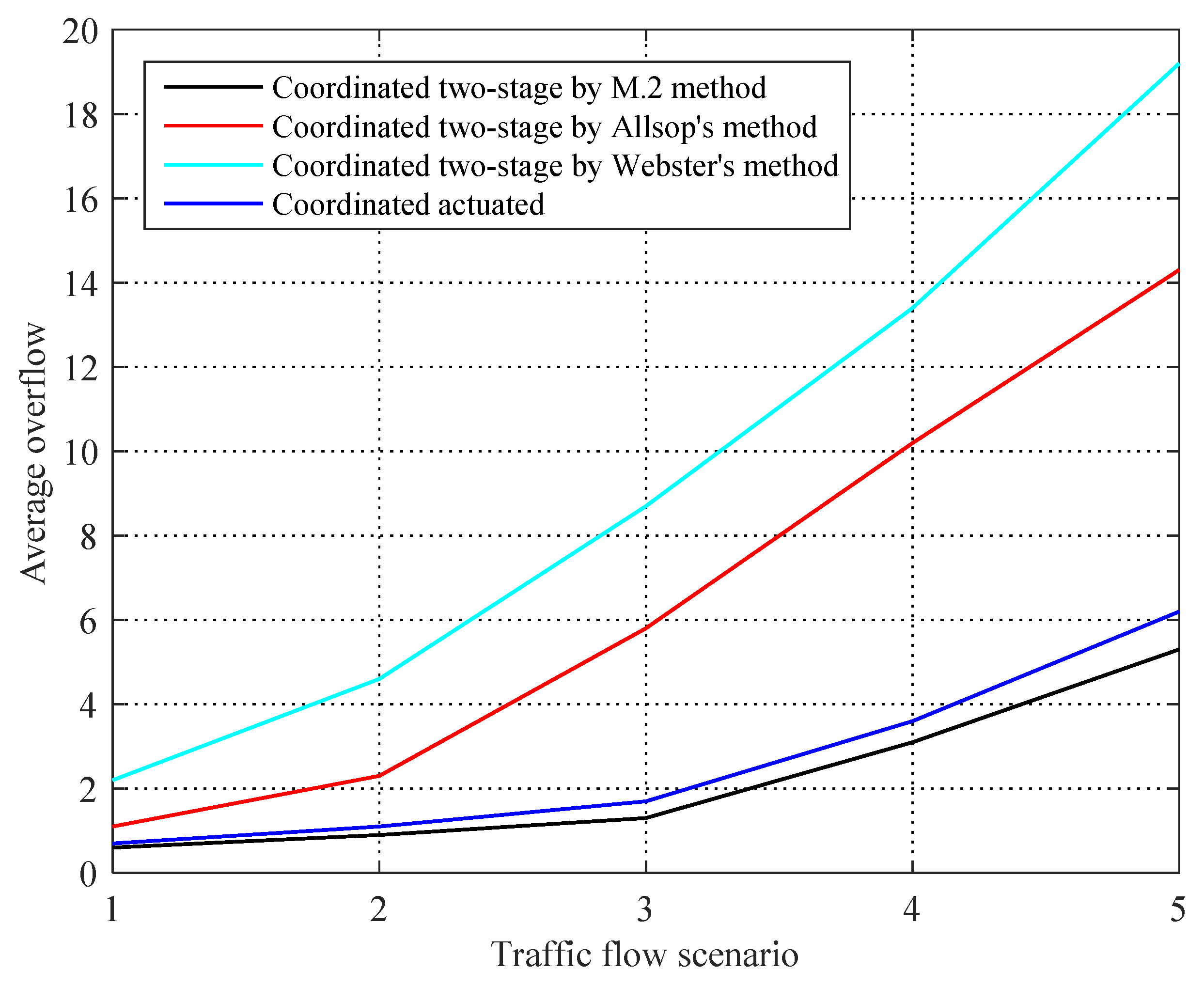
| Traffic Flow Scenario | Control Logic | Method | Phase 1 | Phase 2 | Phase 3 | Avg. Intersection Overflow | |||
|---|---|---|---|---|---|---|---|---|---|
| East | West | East | West | North | South | ||||
| 1 | coordinated two-stage | M.2 | 0.01 | 0.01 | 1.2 | 0.5 | 0.9 | 0.3 | 0.6 |
| Allsop’s | 0.05 | 0.06 | 2.2 | 1.6 | 1.7 | 0.5 | 1.1 | ||
| Webster’s | 0.03 | 0.07 | 5.2 | 2.2 | 4.2 | 1.1 | 2.2 | ||
| coordinated actuated | -- | 0.001 | 0.009 | 2.1 | 0.7 | 2.7 | 0.8 | 0.7 | |
| 2 | coordinated two-stage | M.2 | 0.02 | 0.03 | 2.3 | 1.2 | 1.3 | 0.5 | 0.9 |
| Allsop’s | 0.21 | 0.08 | 8.2 | 5.2 | 2.1 | 1.2 | 2.3 | ||
| Webster’s | 0.15 | 0.1 | 11.3 | 7.2 | 7.3 | 2.3 | 4.6 | ||
| coordinated actuated | -- | 0.002 | 0.028 | 2.8 | 0.9 | 4.2 | 0.9 | 1.1 | |
| 3 | coordinated two-stage | M.2 | 0.03 | 0.05 | 3.2 | 2.1 | 2.6 | 0.6 | 1.3 |
| Allsop’s | 0.3 | 0.4 | 17.5 | 10.3 | 9.5 | 2.4 | 5.8 | ||
| Webster’s | 0.2 | 0.3 | 20.6 | 15.6 | 13.2 | 3.9 | 8.7 | ||
| coordinated actuated | -- | 0.004 | 0.03 | 3.6 | 1.3 | 6.5 | 1.1 | 1.7 | |
| 4 | coordinated two-stage | M.2 | 0.04 | 0.12 | 5.5 | 3.4 | 5.2 | 2.1 | 3.1 |
| Allsop’s | 0.51 | 0.71 | 22.8 | 14.9 | 12.4 | 4.2 | 10.2 | ||
| Webster’s | 0.29 | 0.49 | 29.6 | 20.9 | 19.1 | 7.2 | 13.4 | ||
| coordinated actuated | -- | 0.006 | 0.1 | 6.2 | 1.6 | 9.2 | 1.6 | 3.6 | |
| 5 | coordinated two-stage | M.2 | 0.09 | 0.2 | 7.3 | 6.8 | 8.2 | 3.6 | 5.3 |
| Allsop’s | 0.7 | 0.9 | 32.3 | 21.3 | 17.6 | 6.8 | 14.3 | ||
| Webster’s | 0.6 | 0.7 | 39.2 | 30.4 | 22.3 | 10.3 | 19.2 | ||
| coordinated actuated | -- | 0.008 | 0.15 | 10.1 | 3.2 | 11.8 | 4.2 | 6.2 | |
Disclaimer/Publisher’s Note: The statements, opinions and data contained in all publications are solely those of the individual author(s) and contributor(s) and not of MDPI and/or the editor(s). MDPI and/or the editor(s) disclaim responsibility for any injury to people or property resulting from any ideas, methods, instructions or products referred to in the content. |
© 2023 by the authors. Licensee MDPI, Basel, Switzerland. This article is an open access article distributed under the terms and conditions of the Creative Commons Attribution (CC BY) license (https://creativecommons.org/licenses/by/4.0/).
Share and Cite
Hao, B.; Lv, B.; Chen, Q.; Li, X. A Two-Stage Real-Time Optimization Model of Arterial Signal Coordination Based on Reverse Causal-Effect Modeling Approach. Sustainability 2023, 15, 14035. https://doi.org/10.3390/su151814035
Hao B, Lv B, Chen Q, Li X. A Two-Stage Real-Time Optimization Model of Arterial Signal Coordination Based on Reverse Causal-Effect Modeling Approach. Sustainability. 2023; 15(18):14035. https://doi.org/10.3390/su151814035
Chicago/Turabian StyleHao, Binbin, Bin Lv, Qixiang Chen, and Xianlin Li. 2023. "A Two-Stage Real-Time Optimization Model of Arterial Signal Coordination Based on Reverse Causal-Effect Modeling Approach" Sustainability 15, no. 18: 14035. https://doi.org/10.3390/su151814035
APA StyleHao, B., Lv, B., Chen, Q., & Li, X. (2023). A Two-Stage Real-Time Optimization Model of Arterial Signal Coordination Based on Reverse Causal-Effect Modeling Approach. Sustainability, 15(18), 14035. https://doi.org/10.3390/su151814035