Evaluation of Geospatial Interpolation Techniques for Enhancing Spatiotemporal Rainfall Distribution and Filling Data Gaps in Asir Region, Saudi Arabia

Helmi, Ahmed M.; Elgamal, Mohamed; Farouk, Mohamed I.; Abdelhamed, Mohamed S.; Essawy, Bakinam T.

doi:10.3390/su151814028

Open AccessArticle

Evaluation of Geospatial Interpolation Techniques for Enhancing Spatiotemporal Rainfall Distribution and Filling Data Gaps in Asir Region, Saudi Arabia

¹

Irrigation and Hydraulics Department, Faculty of Engineering, Cairo University, Giza 12613, Egypt

²

Civil Engineering Department, College of Engineering, Imam Mohammad Ibn Saud Islamic University (IMSIU), Riyadh 13318, Saudi Arabia

³

Irrigation and Hydraulics Department, Faculty of Engineering, Ain Shams University, Cairo 11517, Egypt

⁴

Global Institute for Water Security, University of Saskatchewan, Saskatoon, SK S7N 3H5, Canada

⁵

Civil and Infrastructure Engineering and Management Department, Nile University, Sheikh Zayed City 12588, Egypt

^*

Author to whom correspondence should be addressed.

Sustainability 2023, 15(18), 14028; https://doi.org/10.3390/su151814028

Submission received: 23 August 2023 / Revised: 17 September 2023 / Accepted: 20 September 2023 / Published: 21 September 2023

(This article belongs to the Special Issue Hydrological Management Adopted to Climate Change)

Abstract

:

Providing an accurate spatiotemporal distribution of rainfall and filling data gaps are pivotal for effective water resource management. This study focuses on the Asir region in the southwest of Saudi Arabia. Given the limited accuracy of satellite data in this arid/mountain-dominated study area, geospatial interpolation has emerged as a viable alternative approach for filling terrestrial records data gaps. Furthermore, the irregularity in rain gauge data and the yearly spatial variation in data gaps hinder the creation of a coherent distribution pattern. To address this, the Centered Root Mean Square Error (CRMSE) is employed as a criterion to select the most appropriate geospatial interpolation technique among 51 evaluated methods for maximum and total yearly precipitation data. This study produced gap-free maps of total and maximum yearly precipitation from 1966 to 2013. Beyond 2013, it is recommended to utilize ordinary Kriging with a J-Bessel semivariogram and simple Kriging with a K-Bessel semivariogram to estimate the spatial distribution of maximum and total yearly rainfall depth, respectively. Additionally, a proposed methodology for allocating additional rain gauges to improve the accuracy of rainfall spatial distribution is introduced based on a cross-validation error (CVE) assessment. Newly proposed gauges in the study area resulted in a significant 21% CVE reduction.

Keywords:

geospatial interpolation; data gaps; kriging; optimum rainfall locations; arid region

1. Introduction

Arid lands cover 41% of the Earth’s surface and sustain one-third of the global population, half the world’s livestock, and around 44% of its food production [1]. These regions, characterized by low rainfall and high evaporation rates, have witnessed heightened water demand in recent decades, intensifying pressure on freshwater resources and amplifying water scarcity concerns [2,3]. The irregular occurrence of droughts and floods in these areas presents substantial challenges to water resource management [4]. Moreover, optimizing irrigation practices and enhancing crop yields, especially in water-scarce arid regions, relies on a comprehensive understanding of rainfall distribution [5]. Analyzing these patterns facilitates the identification of drought- and flood-prone zones, enabling proactive mitigation strategies. Predicting rainfall in arid regions poses challenges due to intricate interactions among meteorological factors such as air temperature, humidity, and wind, further compounded by the scarcity of comprehensive meteorological networks, which hinders precise assessment efforts [6,7,8,9]. Navigating the sporadic and unpredictable nature of rainfall patterns necessitates the inclusion of additional environmental determinants, such as the topography and elevation of different locations [10,11]. Hence, accurate rainfall measurement and prediction are vital for effective water management in such strategic regions.

The emergence of spatial data and distributed models, coupled with advanced computing capabilities, has collectively led to the integration of these models into scientific research due to their ability to simulate intricate flow regimes within complex study domains [12,13,14]. Factors including spatial rain gauge distribution, elevation, and historical data length contribute to the precision of spatial rainfall estimation at targeted sites. These factors affect the simulation of various hydrological processes like runoff, recharge, soil moisture, and evaporation [4,15,16]. Therefore, ensuring accurate gridded rainfall data is crucial to meet the demands of these models.

Ground truth rainfall records provide valuable insights for calibration, identifying trends and patterns, analyzing the impact of climate changes, and correcting biases in current climatic models and their future projections [17,18]. The number of rain gauges required to obtain accurate rainfall estimates depends on the size of the area under consideration and the desired level of accuracy [6]. Inadequate gauge numbers can result in underestimation or overestimation of rainfall amounts, leading to erroneous conclusions about the water balance within the studied region [19,20]. Challenges are also apparent in data accessibility and limitations, such as brief availability or data gaps, while data reliability may be compromised due to measurement errors or inhomogeneities and potential unavailability [19]. Even with a well-distributed gauge network, some dysfunction during storm events exacerbates the challenges. One potential issue when examining rainfall data involves missing records due to various factors, including discontinued measurements, and damaged/displaced rainfall gauges following flood events, among others. These data gaps can yield false trends or spatial correlations that inaccurately represent natural variations [21,22]. Researchers employ advanced modeling techniques and satellite data to address these challenges and enhance the precision of rainfall prediction in arid regions. These techniques facilitate a comprehensive understanding of the factors influencing rainfall patterns and provide details about spatial distribution [12,14,20,21]. From a hydrological standpoint, assessing the reliability of existing ground truth rain gauges in estimating rainfall data in areas lacking gauge information is pivotal.

The ground rain gauge station network in arid regions exhibits a dual nature, characterized by coarse spacing adhering to World Meteorological Organization (WMO) guidelines for minimum density and historical rainfall data often containing gaps that need filling before use [23]. Several techniques are detailed in the literature to address these gaps, including using satellite data [24,25,26,27], implementing geostatistical interpolation techniques between terrestrial rain gauges to conduct regional rainfall analyses from available data measurements as detailed in Table 1, or using machine learning and statistical analysis [28]. Although satellite-based rainfall estimates can provide valuable information, their limitations in accuracy and spatial resolution emphasize the necessity of ground truth rain gauges and appropriate interpolation methods to improve the accuracy of rainfall estimates. For instance, satellite data have not yet provided a satisfying accuracy for total and maximum yearly precipitation information in the Arabian Peninsula, making geostatistical interpolation between terrestrial rain gauges crucial for obtaining reliable rainfall data [29]. Therefore, it is essential to have an adequate density of rain gauges over the area under consideration to obtain accurate rainfall estimates.

Spatial interpolation techniques are widely utilized to enhance the spatial resolution of data through the estimation of values in areas without sampling, applied in geosciences, water resources, environmental sciences, agriculture, and civil engineering [30,31]. However, their accuracy is influenced by factors such as sampling density, sample spatial distribution, sample clustering, surface type, data variance, data normality, quality of secondary information, stratification, and grid size or resolution [32,33], sometimes resulting in underestimations or overestimations. To enhance accuracy, ground truth gauges are used for calibration in these techniques [18]. The selection of an interpolation method, whether deterministic or geostatistical, depends on the trade-off between accuracy and computational efficiency. Deterministic techniques are more straightforward and faster but do not account for the uncertainty associated with the estimation process [34], while geostatistical techniques provide a comprehensive view of the uncertainty associated with the estimation process but are computationally more intensive [35,36]. As a result, several spatial interpolation techniques have been developed that are appropriate for the rapid estimation process [20,37,38,39,40,41].

To evaluate the efficiency of spatial interpolation techniques, it is imperative to consider the following key factors: (1) the design of the sampling process; (2) the mean and coefficient of variation of the primary variable for either the estimation dataset or validation dataset; (3) the sample size for both the estimation and validation datasets; (4) the geographical extent of the study area; and (5) the use of appropriate accuracy measurements [31]. Studies have analyzed spatial interpolation techniques (see Table 1); however, comprehensive conclusions remain elusive. Despite this, the three most frequently compared techniques are Ordinary Kriging (OK), Inverse Distance Weighting (IDW) with inverse distance squared (IDS), while different types of Kriging geostatistical techniques were evaluated: Ordinary Kriging, Cokriging, and Empirical Bayesian Kriging.

Table 1. Sample of available comparative studies in the literature.

Interpolation Method	Validation Method	Recommended Method	Ref.
Thiessen Polygon (TB), Inverse Distance Weighting (IDW), Linear Regression (LG), Kriging with External Drift (KED), Ordinary Kriging (OK)	Root Mean Squared Error (RMSE)	Ordinary Kriging (OK)	[42]
Inverse Distance Weighting (IDW), Local Polynomial Interpolation (LPI) Global Polynomial Interpolation (GPI) Simple Kriging (SK) Universal Kriging (UK), Ordinary Kriging (OK), Radial Basis Function (RBF)	Mean Error (ME) Root Mean Squared Error (RMSE)	Ordinary Kriging (OK)	[43]
Natural Neighbor Interpolation (NNI), Ordinary Kriging (OK) Cokriging (CK)	Root Mean Squared Error (RMSE)	Cokriging (CK)	[44]
Kriging with External Drift (KED), Optimal Interpolation Method (OIM), Thiessen Polygons (TB)	Root Mean Squared Error (RMSE)	Optimal Interpolation Method (OIM)	[45]
Inverse Distance Weighting (IDW), Radial Basis Function (RBF), Diffusion Interpolation with Barrier (DIB), Kernel Interpolation with Barrier (KIB), Ordinary Kriging (OK), Empirical Bayesian Kriging (EBK)	Leave-One-Out Cross-Validation (LOOCV), Mean Square Error (MSE), Mean Absolute Error (MAE), Mean Absolute Percentage Error (MAPE), Symmetric Mean Absolute Percentage Error (SMAPE) Nash–Sutcliffe Efficiency Coefficient (NSE)	Kernel Interpolation with Barrier (KIB)	[46]
Inverse Distance Weighting (IDW), Radial Basis Function (RBF), Local Polynomial Interpolation (LPI), Global Polynomial Interpolation (GPI), Simple Kriging (SK), Universal Kriging (UK), Ordinary Kriging (OK), Empirical Bayesian Kriging (EBK), Empirical Bayesian Kriging Regression Prediction (EBKRP)	Mean Error (ME), Root Mean Square Error (RMSE), Pearson R2 (R2), Mean Standardized Error (MSE), Root Mean Square Standardized Error (RMSSE), Average Standard Error (ASE)	Empirical Bayesian Kriging Regression Prediction (EBKRP)	[47]
Inverse Distance Weighting (IDW), Kriging, ANUDEM, Spline	Mean Absolute Error (MAE), Mean Relative Error (MRE), Root Mean Squared Error (RMSE), Spatial and Temporal Distributions.	Inverse Distance Weighting (IDW)	[48]
Inverse Distance Weighting, Natural Neighbor (NN), Regularized Spline (RS), Tension Spline (TS), Ordinary Kriging (OK), Universal Kriging (UK)	Root Mean Square Error (RMSE), Mean Absolute Error (MAE), Mean Bias Error (MBE), Coefficient of Determination (R2)	Ordinary Kriging (OK)	[49]
Inverse Distance Weighting (IDW), Ordinary Kriging (OK), Ordinary Cokriging (OCK), Linear Regression (LR), Simple Kriging with varying Local Means (SKLM), Kriging with an External Drift (KED)	Mean Error (ME), and Root Mean-Square Error (RMSE)	Ordinary Cokriging (OCK)	[50]
Circular Ordinary Kriging (COK), Spherical Ordinary Kriging (SOK), Exponential Ordinary Kriging (EOK), Gaussian Ordinary Kriging (GOK), Empirical Bayesian Kriging (EBK)	Mean Error (ME), Mean Standardized Error (MSDE), Root Mean Square Standardized Error (RMSSDE) Mean Standard Error (MSE), Root Mean Square Error (RMSE)	Exponential Ordinary Kriging (EOK), Empirical Bayesian Kriging (EBK)	[51]

Saudi Arabia ranks among the arid countries confronting challenges in accurately predicting rainfall patterns [4]. Therefore, this study aims to rectify the lack of rainfall data in an arid region, the Asir area in Saudi Arabia, to provide a reliable and accurate spatial distribution of rainfall. The objectives of this study encompass:

Assessing various spatial interpolation techniques to ascertain the optimal approach for accurate rainfall prediction across diverse arid regions.
Analyzing the sufficiency of rainfall station distribution and pinpointing optimal sites for installing new rain gauges within the study area.
Providing an illustrative example elucidating the practical utilization of study outcomes in filling data gaps at any location and time within the study area for end-users.

In this study, we collect rain gauge data for the Asir Province; however, some gauges lack rainfall records for certain years. As such, we first apply various spatial interpolation techniques to fill in the gap of the missing data for these gauges. Subsequently, we review the distribution of rain gauge stations to determine their sufficiency and determine if more meteorological stations are necessary for specific spots. Ultimately, we suggest the optimal locations for installing additional meteorological stations to improve data collection. The remainder of the article is organized as follows: Section 2 outlines the study area and its characteristics. Section 3 presents the materials and methods. Section 4 reports the main results and discussion of the findings. Section 5 demonstrates a use case to help end-users apply the findings in practical situations, and the article ends with a summary and conclusions in Section 6.

2. The Study Area

The Kingdom of Saudi Arabia (KSA) is the world’s 13th largest country, with an area of about 2,150,000 square kilometers [52,53]. The KSA extends between coordinates 33.75:56.25 E and 16.5:32.5 N, WGS84, and covers roughly 80% of the Arabian Peninsula [54]. The KSA overlooks both the Arabian Gulf and the Red Sea, boasting 550 and 2250 km of shoreline, respectively. These water bodies serve as the kingdom’s primary sources of water vapor [55]. The KSA has a complex topography that can be classified into four categories: (1) coastal plains, (2) central and northern plateaus, (3) the central Tuwayq mountains, and (4) the western Asir mountains. Topographical elevations ascend steeply from the Red Sea shoreline towards the southwestern Asir mountains, reaching the kingdom’s highest value at 2990 m above mean sea level [56]. The location and topography of the KSA are shown in Figure 1.

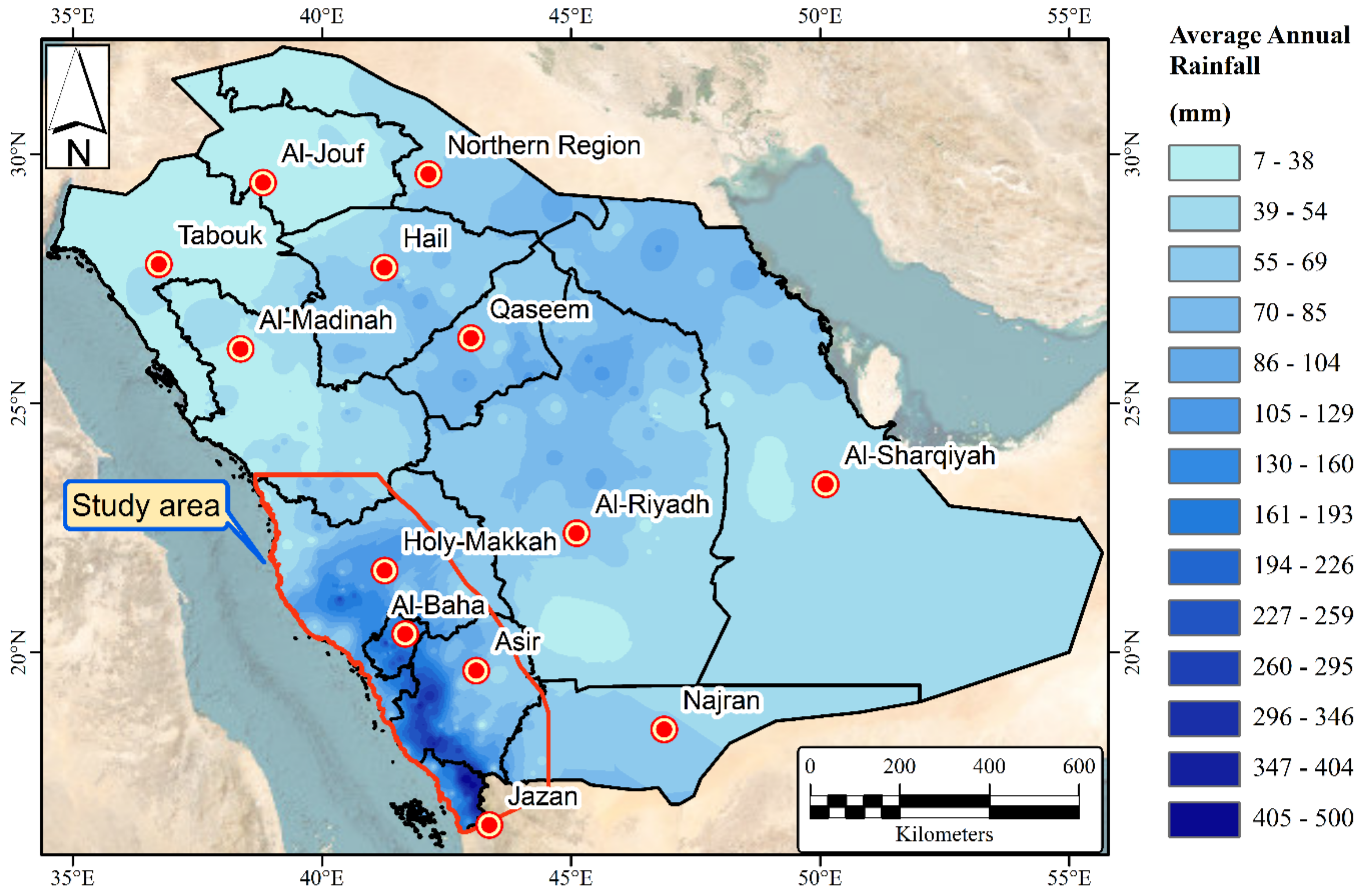
The KSA is predominantly categorized into arid and semi-arid regions [57,58]. Given its prevailing arid climate and limited water resources, only five percent of cultivable land is utilized [59]. Notably, the majority of rainfall events occur between October and April [60]. Figure 2 shows the spatial distribution of the average annual rainfall over the KSA, obtained from available rain gauge records [29]. The southwestern KSA region has the highest potential of harnessing rainfall as a water resource [60]. This region’s mountainous terrain and complex topography generate orographic (convectional) rains, making it an ideal location for water resource exploitation [57,61,62]. Aligned with the World Bank’s recommendations for addressing physical water resource scarcity within the MENA region [63], the area highlighted in Figure 2 was selected as the study area for this study.

3. Materials and Methods

3.1. Rain Gauges

Assessing the adequacy of the rain gauge amount and distribution is the backbone of accurate quantification of rainfall volume. This imperative evaluation becomes particularly pronounced within mountainous terrains, owing to the pronounced spatial disparities in rainfall patterns. The available terrestrial rainfall data used in the current study were collected from official KSA authorities—the Ministry of Environment of the KSA (ME), the Ministry of Water and Agriculture of the KSA (MEWA), and the Presidency of Meteorology and Environment of the KSA (PME). Different types of rainfall gauges are available in the KSA: (1) meteorological (recording) gauges, (2) daily rainfall gauges, (3) recording rainfall gauges, and (4) totalizing rainfall gauges [64]. Within the geographical scope of this study, a total of 128 rain gauge data were acquired, as shown in Figure 3A. Notably, the available records obtained from totalizing gauges exhibit non-uniform temporal intervals, which can restrict their effectiveness in providing accurate estimates for interpreting/analyzing daily or yearly records. Five totalizing gauges are located in the study area, as highlighted in Figure 3B. Based on this criterion, the remaining 123 gauges were selected for the current study, as shown in Figure 3C. The study area has significant variability in altitude among its rain gauges, from 0 to 2603 m above mean sea level, as illustrated in Figure 3D. The properties of the selected rain gauges are summarized in Table 2, including the number of records available between the first and last available dates, as well as any missing yearly records (data gaps) during that period. Inconsistency can be noted in the available rain gauge data due to the randomness in rainfall patterns and the spatial variability in the missing data locations in the available time frame. Figure 4 shows the temporal variation in the 123 selected gauges. To perform a geostatistical analysis in the study area, a threshold of at least 50 rain gauge data points was chosen. This threshold was met, allowing for a 48-year analysis period from 1966 to 2013. However, there are gaps in the rainfall records that need to be predicted with an appropriate interpolation method.

3.2. Interpolation Techniques

The characteristics of available datasets influence the spatial interpolation outcomes, so selecting an accurate interpolation method is a crucial part of generating accurate distribution rainfall maps. Until recently, most of the studies in this field provided a limited comparison of interpolation techniques, relying on statistical errors to select the best method. The choice of interpolation method depends on the nature of the data, the size of the study area, and the desired level of accuracy. Each method has its pros and cons, and it is important to choose the most appropriate one for a specific application [65].

The selected spatial interpolation techniques were systematically analyzed to determine their accuracy in estimating unknown rainfall values and predicting the spatial rainfall distribution pattern. In the current study, the authors selected to evaluate two different interpolation categories, i.e., deterministic and geostatistical. Nearly all commonly known interpolation techniques and various models within these techniques were analyzed to determine the most optimal method for interpolating rainfall data in the study area.

Four interpolation techniques were evaluated under the deterministic technique umbrella: Inverse Distance Weighting (IDW), Global Polynomial Interpolation (GPI), Radial Basis Functions (RBF), and Local Polynomial Interpolation (LPI). Additionally, three interpolation techniques under the geostatistical technique umbrella were also evaluated, which were the Kriging, Cokriging, and Empirical Bayesian Kriging (EBK), with seven different semivariogram models such as Circular, Spherical, Exponential, Gaussian, K-Bessel, J-Bessel, and Stable models. The interpolation techniques’ mathematical equations are given in Appendix A.

Generally, 51 interpolation techniques (43 geostatistical and 8 deterministic) were selected to be assessed in the current study to determine the most suitable interpolation technique for the data available, as shown in Table 3.

3.2.1. Deterministic Techniques

The Inverse Distance Weighting (IDW) method estimates the value of the target point based on the values of neighboring points, with more weight given to points closer to the target point. The IDW method uses the Cartesian coordinates of the target station and uses the inverse distance raised to a power P as a weighting factor for the adjacent points values, as shown in Equation (1) [31,33,34,36,42]. According to this method, the influence of a variable diminishes with the distance from its sampled location. Using a high power in IDW emphasizes the nearest points, and creates a more detailed surface with lower smoothness [66]. Five IDW interpolation powers were tested in the current study, namely IDWP1, IDWP2, IDWP3, IDWP4, and IDWP5, for P = 1, 2, 3, 4, and 5, respectively.

z_{p} = \frac{\sum_{i = 1}^{n} (\frac{z_{i}}{d_{i}^{p}})}{\sum_{i = 1}^{n} (\frac{1}{d_{i}^{p}})}

(1)

where

z_{i}

is the known value point, di is the distance to a known point,

z_{i}

is the unknown point, and p is the exponent power (1, 2, 3, 4, or 5) [67].

Global Polynomial Interpolation (GPI) is a mathematical technique that can calculate a polynomial function to pass through a set of given points. GPI is a highly accurate tool in numerical analysis and can be used to estimate any continuous function. The key advantage of GPI over other interpolation techniques is that it provides a single polynomial function to approximate the entire curve instead of several piecewise functions. To perform GPI, a set of points that lie on the curve to be estimated must be chosen, and a polynomial function is then constructed to pass through these points. The degree of the polynomial is determined by the number of points selected. Higher-degree polynomials can provide more accurate approximations, but they may also be more prone to rounding errors and other factors. GPI is a fast and global method of predicting rainfall based on the polynomial function [66,68]. The second-degree polynomial is selected for the current study.

The Radial Basis Function (RBF), also known as the Spline method, uses artificial neural networks (ANN) to accurately interpolate data. The RBF is a popular tool for interpolating multi-dimensional scattered data and can be easily generalized to various space dimensions, making it useful in natural resource management. In addition to acting as a class of interpolation techniques for georeferenced data, the RBF is a deterministic interpolator that utilizes the level of smoothing to determine the appropriate interpolation technique [68,69].

Local Polynomial Interpolation (LPI) is a method for approximating a function by fitting a polynomial to small subsets of the data. This technique involves constructing a locally best-fitting polynomial to a set of points, rather than fitting a single polynomial to all the points globally. LPI is particularly useful when dealing with large datasets or highly variable functions. By considering the local behavior of the data, it allows for a more accurate representation of the function. In addition, LPI can estimate derivatives and integrals of the function at specific points [68].

3.2.2. Geostatistical Techniques

Geostatistics is a statistical technique that deals with spatially distributed variables. Its original purpose was to predict the likelihood of finding gold ore in the Witwatersrand mine in South Africa [70]. This technique employs a semivariogram, which describes the spatial correlation between data points, to estimate values at locations where no samples exist. The semivariogram, which plots the variance of the differences between pairs of points against their spatial separation, is vital to geostatistical interpolation. It is used to model the spatial dependence of the estimated variables and to interpolate values at unsampled locations. The semivariogram provides information about the spatial correlation between data points and is used to estimate the weights that are applied to the measured values of the variable being estimated at unsampled locations [68].

Kriging is a widely used technique in the fields of geology, environmental science, and engineering to estimate the value of a variable at an unobserved location based on nearby observed locations. The technique relies on spatial autocorrelation, which refers to the tendency of locations to exhibit similar values to the given variable. Kriging utilizes this principle to estimate the variable’s value at an unobserved location by analyzing the spatial correlation between nearby observed locations. This involves fitting a mathematical model to the observed data, which describes the spatial correlation between data points. The resulting model is then used to estimate the variable’s value at the unobserved location by taking a weighted average of the values of the variable at nearby observed locations, with the weights assigned based on the spatial correlation between the locations [21,31,33,42]. Kriging offers several benefits over other interpolation techniques, including more accurate estimates and a measure of uncertainty for each estimate. This can be particularly useful in decision-making processes, where a clear understanding of the accuracy and reliability of the estimates is critical. The semivariogram is a mathematical function used to describe the spatial autocorrelation of a variable and is used to measure the degree to which the values of the variable at two locations are similar as a function of the distance between these locations.

Cokriging is a variation of Kriging that enables the inclusion of additional spatially correlated variables in the estimation process. This method enhances the precision of rainfall estimations by considering the connection between rainfall and other factors such as elevation, temperature, and land use. It is particularly beneficial when the rainfall data are limited or unreliable. The Cokriging method assesses the cross-covariance function between two variables, describing their spatial correlation. It then uses this function to determine the weights to be assigned to the measured values of the related variable to predict the rainfall values at unsampled locations. Cokriging is a valuable tool for spatially analyzing rainfall, improving our understanding and prediction of rainfall patterns [71,72].

Empirical Bayesian Kriging (EBK) is a geostatistical interpolation method used to estimate rainfall distribution in spatial domains. It tackles some challenges present in spatially valid Kriging models, such as the manual adjustment of parameters required by other Kriging techniques. Instead, EBK automates the parameter calculation process by combining submissions and simulations [73,74,75]. EBK stands out from other Kriging techniques due to its ability to account for errors arising from semivariogram estimation. It employs a hierarchical Bayesian model that incorporates prior semivariogram knowledge, enhancing the accuracy of interpolated values by reducing the estimation errors. This flexible approach yields accurate estimates, especially with limited data. The EBK process includes estimating a semivariogram model from available data, simulating new values at input locations based on this model, and iteratively estimating new semivariogram models from simulated data. This produces a spectrum of semivariograms, enabling prediction and standard error computation for unsampled locations. In contrast to classical Kriging, EBK optimizes parameters differently. It automatically refines parameters using diverse semivariogram models, resulting in enhanced adaptability and estimate accuracy [73,74,75].

4. Results and Discussion

Automation of geostatistical analysis in Arc-GIS via template parameters can be incorporated into deterministic and geostatistical approaches that do not require semivariograms. Seven types of semivariograms (i.e., Circular, Spherical, Exponential, Gaussian, K-Bessel, J-Bessel, and Stable) were selected to be evaluated within Kriging and Cokriging techniques and their sub-types (i.e., ordinary, simple, and universal). A semivariogram relates the distance between rain gauge locations and the variance between rain gauge records. Consequently, the semivariogram varies from year to year based on available records. These variances and inability to automate the process necessitate the manual generation of 4032 geostatistical parameters for Kriging and Cokriging through the 48-year study period (2 (Kriging and Cokriging) × 3 (Kriging types) × 7 (semivariogram types) × 48 (number of years)). For other interpolation techniques, parameter values (e.g., the power of the IDW) were defined once and repeated for each year of the study period.

Several quantitative statistical metrics are found in the literature, offering different lenses for evaluating the accuracy of interpolation techniques. The Mean Absolute Error (MAE: Equation (2)) measures the average error between predicted

(P_{i})

and measured rainfall values

(M_{i})

. The Root Mean Square Error (RMSE: Equation (3)) calculates the standard deviation of the errors. The Centered Root Mean Square Error (CRMSE: Equation (4)) disregards the mean values in the error evaluation. Taylor’s graphical plot (Taylor, 2001) provides valuable information about the standard deviation, the correlation coefficient (CC: Equation (5)), and CRMSE for

(M_{i})

and

(P_{i})

.

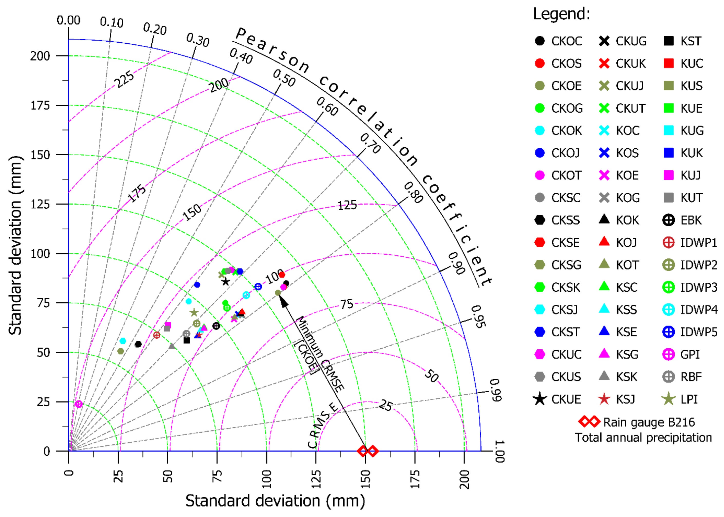
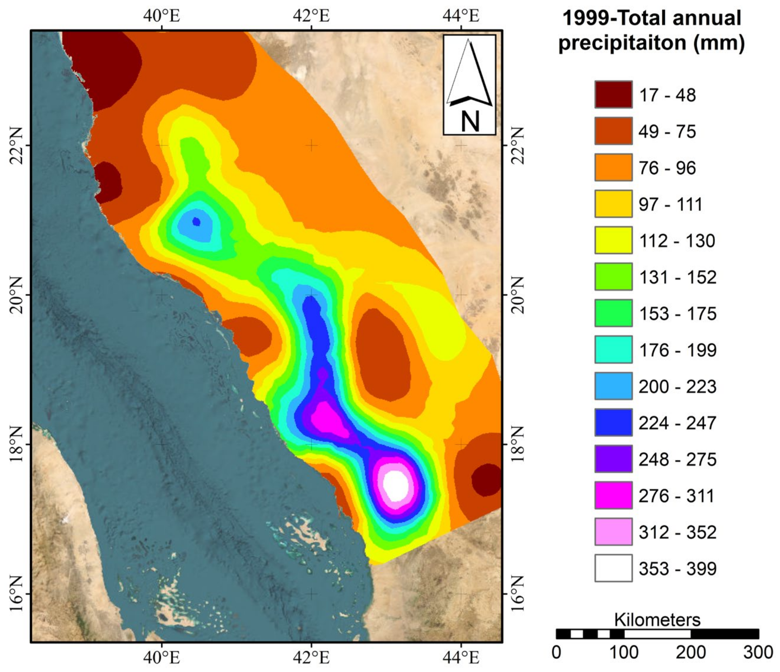
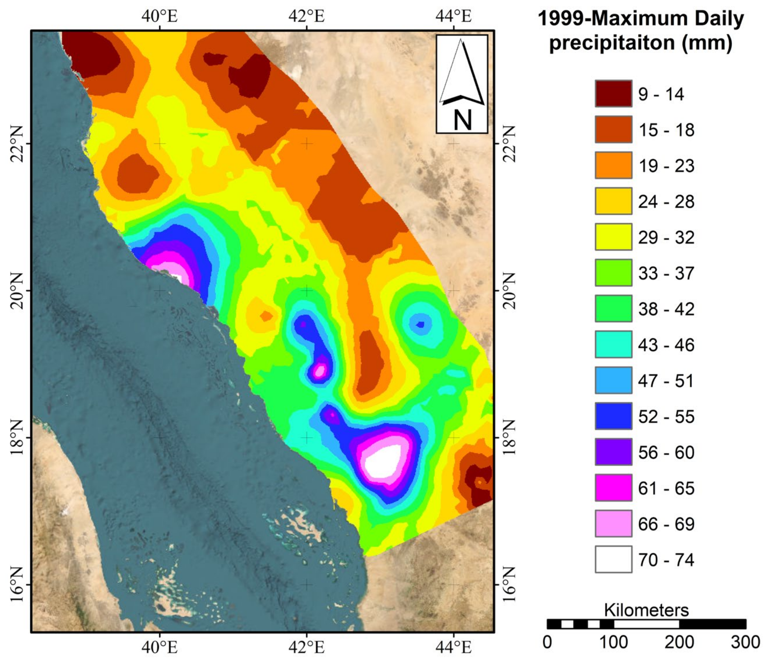
In this study, the cross-validation CRMSE serves as the criterion for comparing the prediction accuracy across different geostatistical approaches, guiding the selection of the appropriate technique with the least CRSME. This cross-validation procedure was sequentially conducted across all the points used to generate a geostatistical layer. After omitting each measured value from the dataset, the error at each point was determined by the difference between the predicted and the measured values at the respective location. Across the study period, distinct geostatistical approaches were assigned to each year, addressing total yearly and maximum daily rainfall data. This variation in the appropriate geostatistical approaches is due to the differences in the available rain gauges used to create the dataset from one year to another. Figure 5 shows the Taylor diagram for total yearly rainfall in the study area for the year 1998. Among the approaches, ordinary Cokriging with an exponential variogram (CKOE) emerged with the least centered Root Mean Square Error and thus was selected to generate the total yearly surface for the study area. Similarly, for the year 1999, the spatial distribution of the total annual and maximum daily rainfall depths over the study area based on the selected (CKSG and CKOC) interpolation techniques is given in Figure 6 and Figure 7, respectively. Table 4 shows the yearly selected interpolation techniques for the maximum daily and total annual rainfall over the study area.

MAE = \frac{\sum_{i = 1}^{N} |(M_{i} - P_{i})|}{N}

(2)

RMSE = \sqrt{\frac{1}{N} \sum_{i = 1}^{N} {(M_{i} - P_{i})}^{2}}

(3)

CRMSE = \sqrt{\frac{1}{N} \sum_{i = 1}^{N} {[(M_{i} - \bar{M}) - (P_{i} - \bar{P})]}^{2}} = \sqrt{σ_{M}^{2} + σ_{P}^{2} - 2 \cdot σ_{P} \cdot CC}

(4)

CC = \frac{\sum_{i = 1}^{n} (M_{i} - \bar{M}) \cdot (P_{i} - \bar{P})}{\sqrt{\sum_{i = 1}^{n} {(M_{i} - \bar{M})}^{2}} \cdot \sqrt{\sum_{i = 1}^{n} {(P_{i} - \bar{P})}^{2}}}

(5)

where

μ_{S}

and

σ_{S}

are the mean and standard deviation of satellite rainfall data.

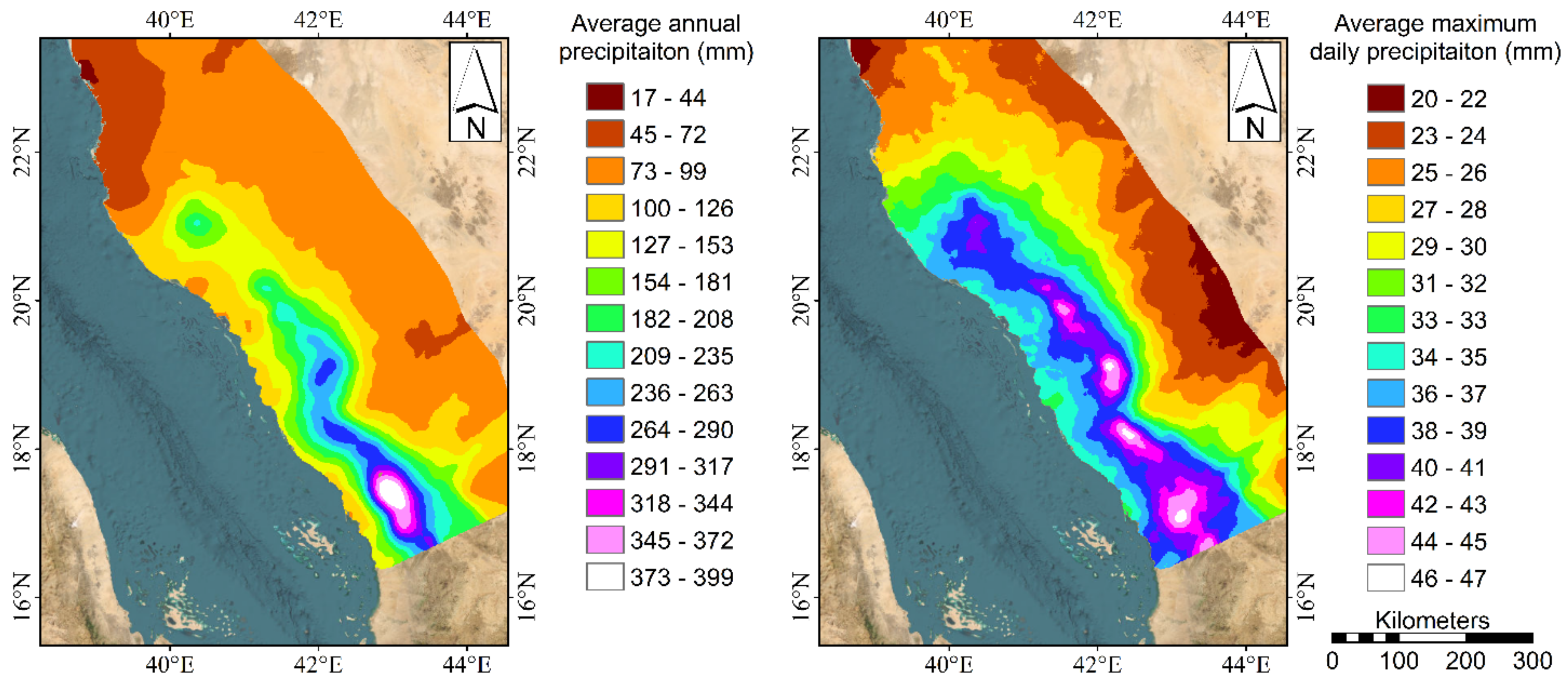
The yearly spatial distribution for maximum and total precipitation over the study area with gaps filled from 1966 to 2013 is given in Figure S1 through Figure S12 in the Supplementary Materials. These rasters can be utilized to directly select any missing data at a specific gauge within the study area boundaries and during the study period (as shown in the use case section). The average values of the total and maximum yearly precipitation were calculated based on the filled data from 1966 to 2013, as given in Figure 8. These average values were utilized to select the optimal interpolation technique in light of the limited availability of rainfall data beyond 2013 due to the limited rain gauge records in this period. In such cases, the Ordinary Kriging with J-Bessel semivariogram (KOJ) and Simple Kriging with K-Bessel (KSK) semivariogram techniques are recommended to fill data gaps for maximum and total yearly precipitation, respectively, for the years after 2013.

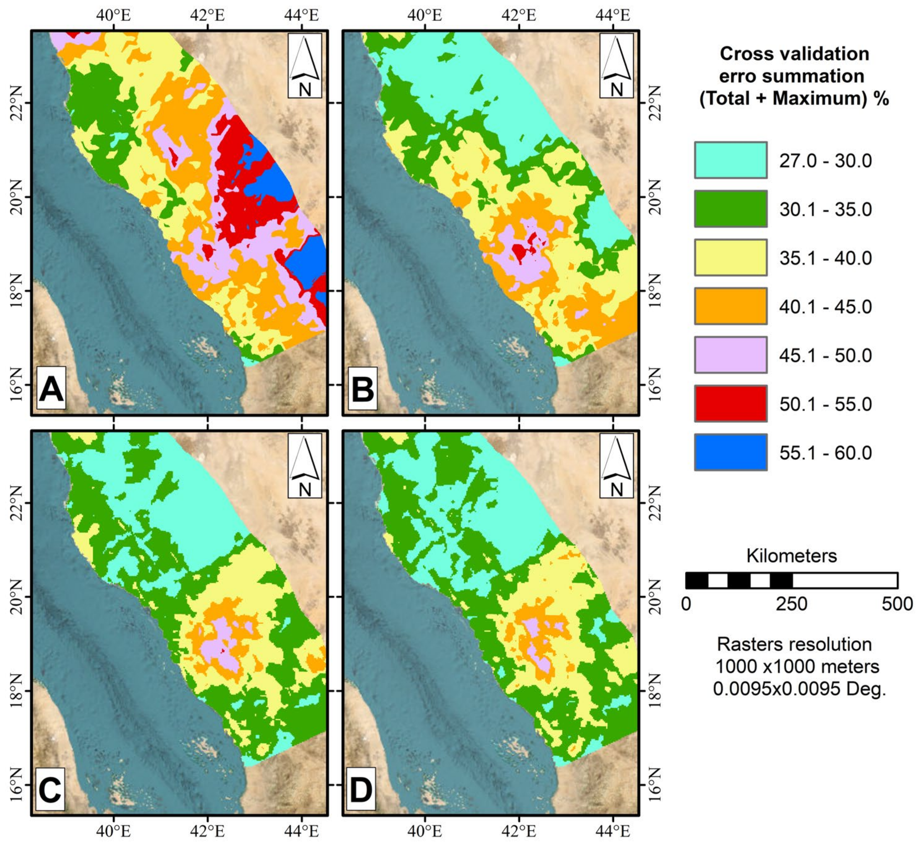
The World Meteorological Organization (WMO) recommends certain densities of rain gauge stations to be followed for different types of catchments. For mountainous regions with irregular rainfall, a density of 250 km² per station is recommended for daily-recording gauges [23]. The density of the rain gauges in the study area is far beyond these recommended limits. Additionally, several publications have discussed different techniques for assessing and optimizing the locations of rain gauge stations and the spatial distribution of the network. These techniques include statistical covariance [76], the Kriging interpolation method, and Kriging and entropy techniques for rainfall network design [77]. In this study, the cross-validation error (CVE) is used as a quality indicator to evaluate the density of a given rain gauge network. The spatial distribution of the CVE for the global proposed maximum daily and total yearly interpolation techniques (KOJ, KSK) is displayed in Figures S13A and S14A in the Supplementary Materials, with the sum of both errors shown in Figure 9A. The maximum combined CVE resulting from the sum of the total rainfall and the maximum rainfall is greater than 50%. The highest CVE is observed in the southeastern part of the study area, likely due to orographic effects. The average of the combined CVE is 42%, as highlighted in Table 5.

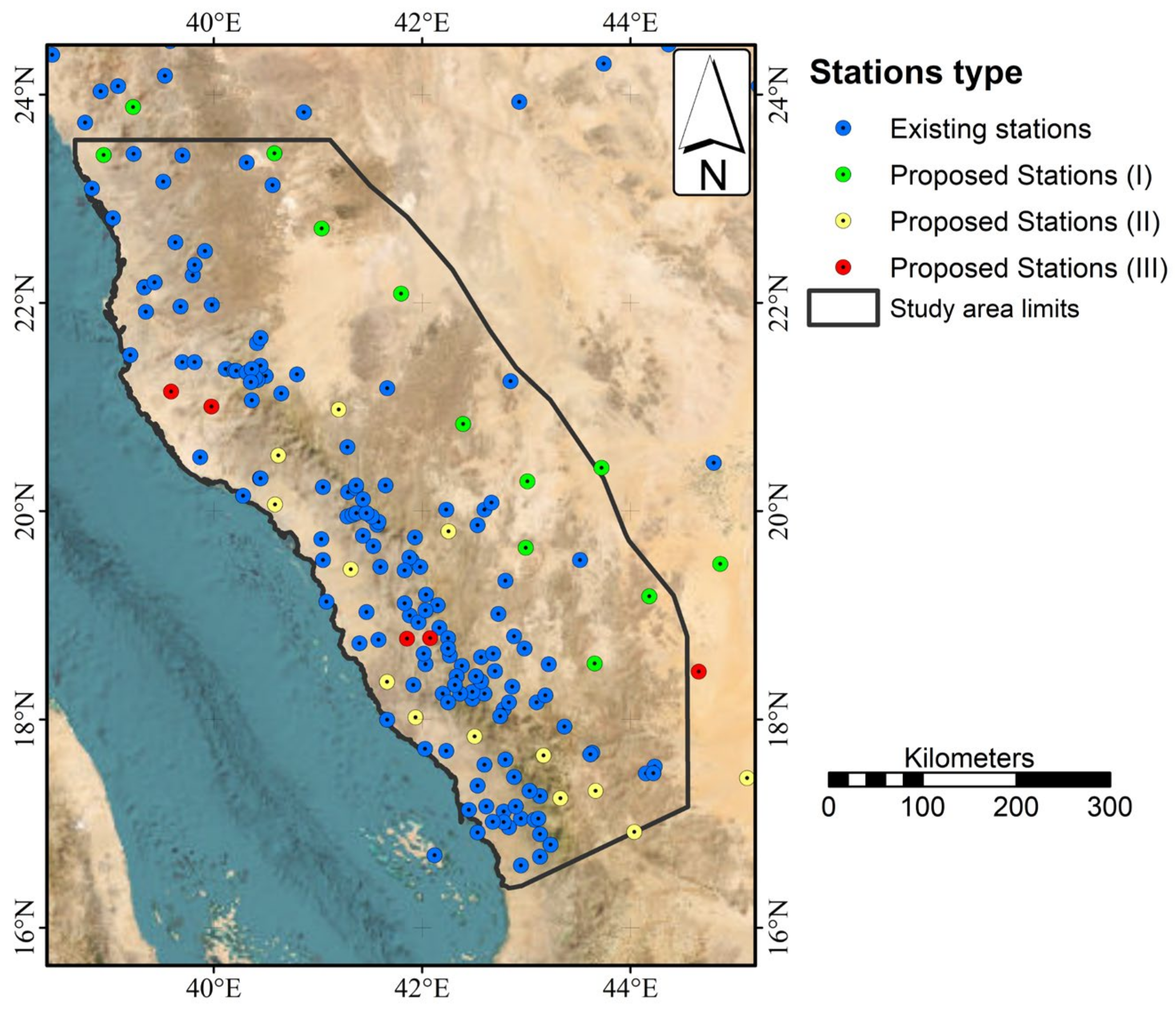
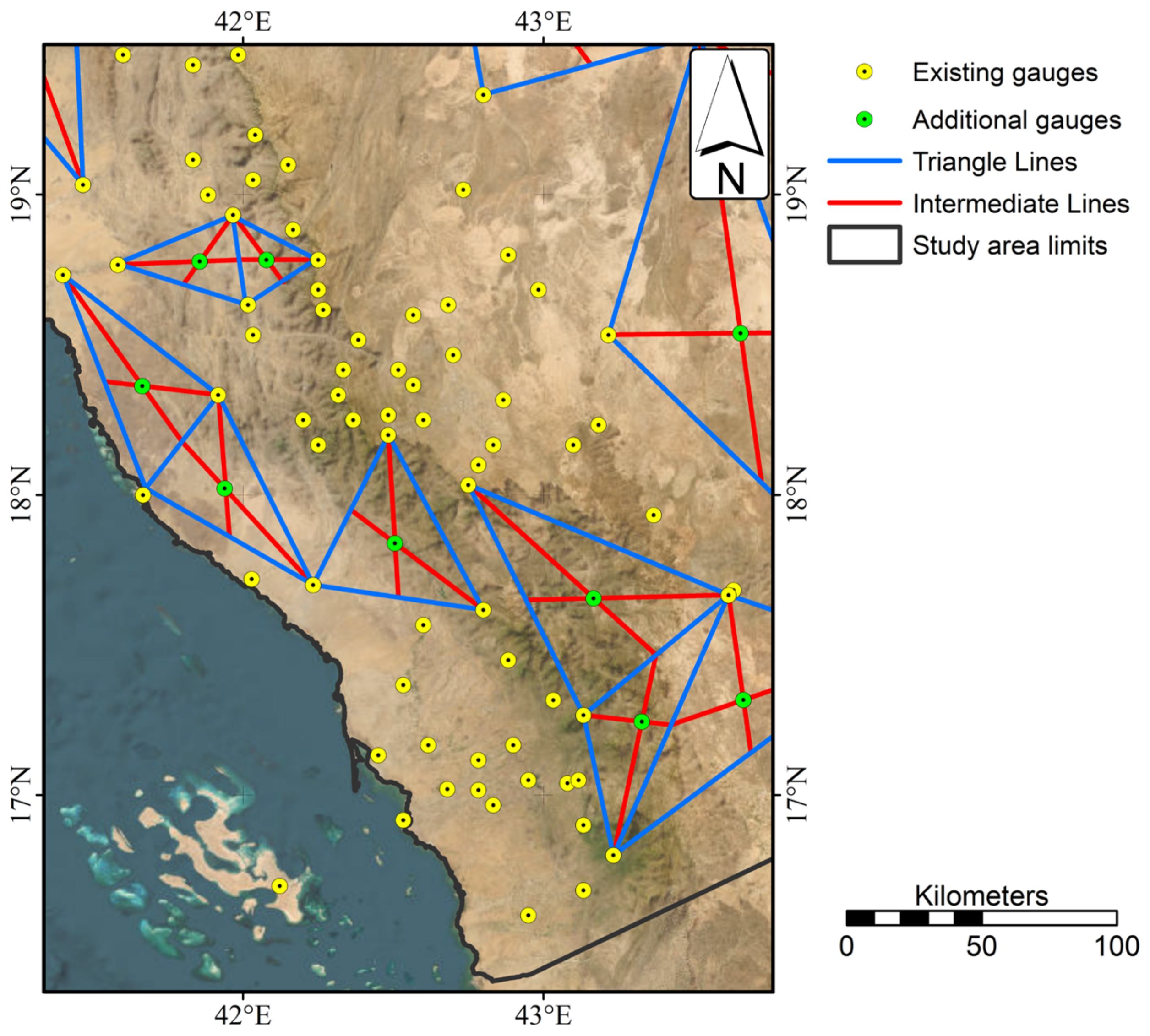
Three additional groups of rain gauges (I, II, and III) are proposed to reduce the CVE, resulting in a total of 135, 148, and 153 stations, respectively, as shown in Figure 10. The proposed locations of the additional rain gauges are identified based on three criteria: (1) areas with the highest cross-validation error, (2) areas with a low rain gauge density, and (3) the proposed locations should be selected to avoid screening other stations located at centroid of the triangle formed by the three closest gauges. Figure 11 demonstrates the proposed methodology for locating new stations.

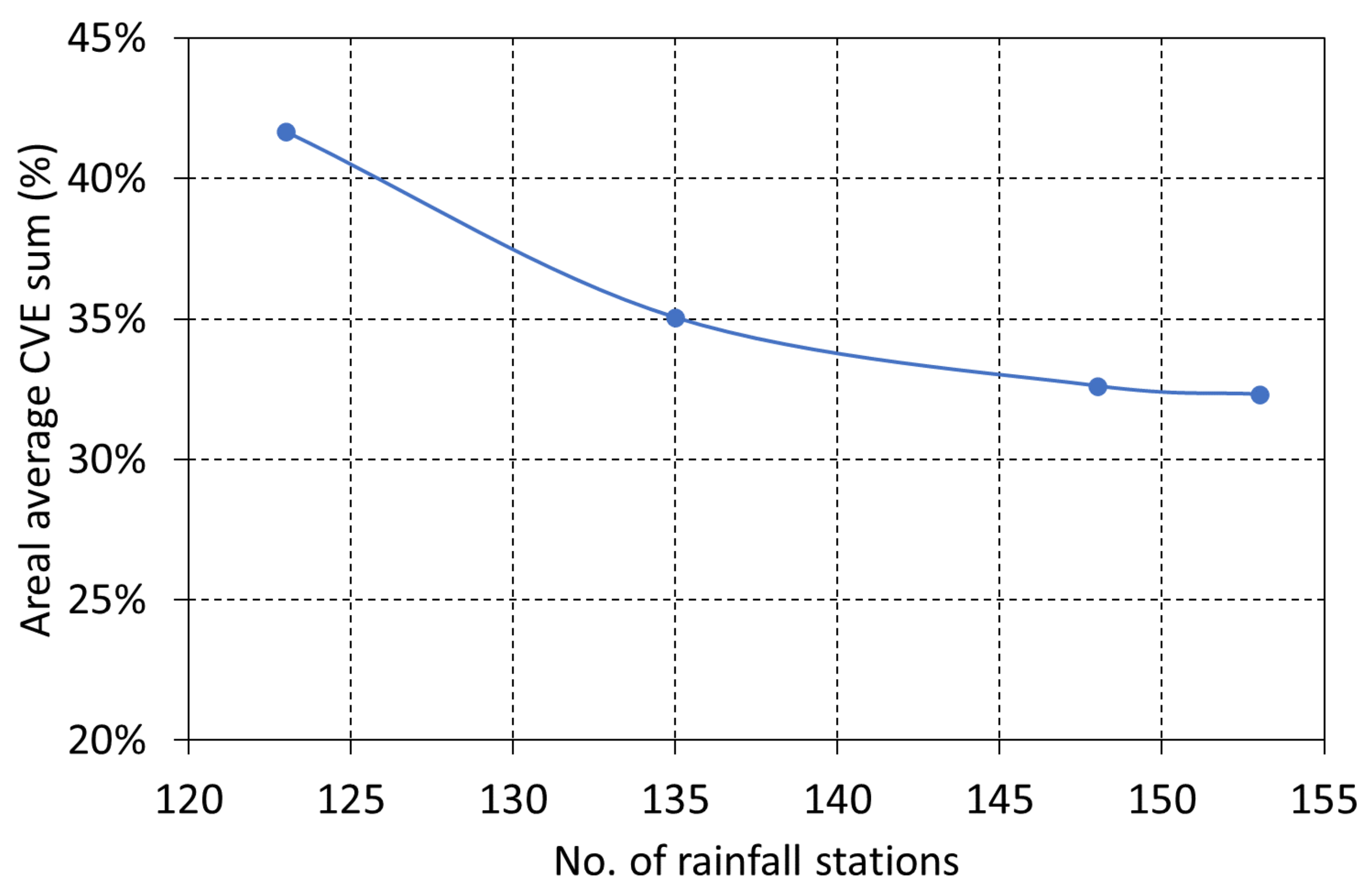
Table 5 shows that adding new candidate stations generally helped to decrease the average CVE. It is interesting to note that this reduction in CVE is not linear, as shown in Figure 12. Increasing the existing rain gauge stations by 10% (group I) resulted in a decrease in the average CVE by 16%. However, the additional addition of 10% of the number of rain gauge stations from group I to group II resulted in a decrease of less than 6% in the average CVE.

Assessing and categorizing the aridity in different climatic regions have significant implications for agricultural productivity, water resource management, and environmental conservation. The United Nations Environment Programme (UNEP) introduced the Aridity Index (AI) as a quantitative measure of aridity, involving the evaluation of the ratio of annual rainfall (P) to potential evapotranspiration (PET) [78]. The aridity is classified as desert, hyper-arid, arid, semi-arid, dry subhumid, or subhumid based on the AI values shown in Table 6 [79]. Hyper-arid regions receive minimal rainfall. Arid regions have insufficient rainfall to sustain vegetation and semi-arid regions experience slightly higher but still inadequate rainfall, while dry, sub-humid regions receive enough rainfall to support continuous harvesting without requiring irrigation.

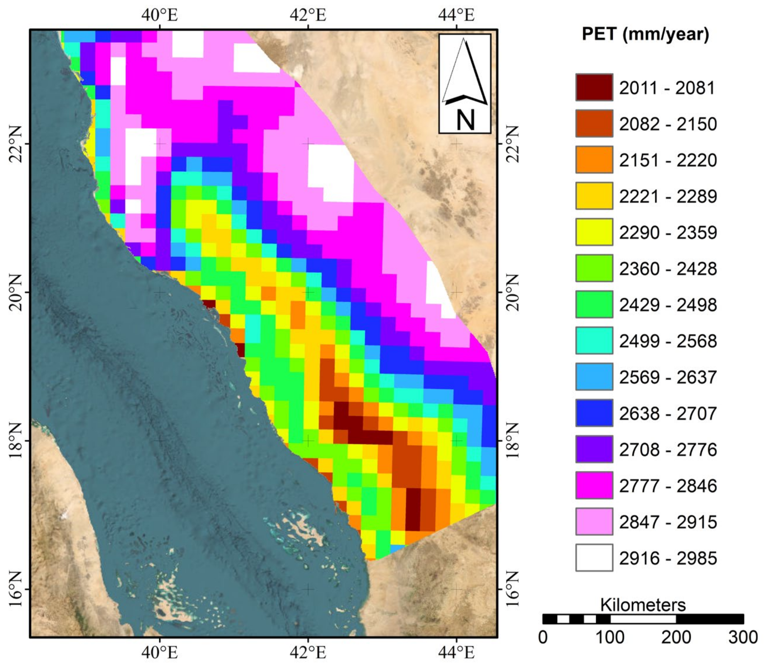
To determine the AI within the study area, it was necessary to determine the average annual rainfall and PET values. Figure 8 shows that the time-averaged annual rainfall varies from a minimum of 17 mm/year (at the northwestern boundary of the study area) to less than 400 mm/yr (in the mountainous southern region). Annual PET data were acquired from the publicly accessible WaPOR portal, developed by the Food and Agriculture Organization [80]. The WaPOR portal offers a near real-time database utilizing satellite data, facilitating the monitoring of agricultural water productivity across various spatial scales. The dataset obtained from the WaPOR database comprised multiple resolution levels: continental (250 m ground resolution), country (100 m), and sub-national (30 m). This dataset encompasses several variables, including water productivity, land productivity, actual and potential evapotranspiration, land cover and use, biomass, rainfall, carbon dioxide uptake, yields, harvested index, and crop calendar. For this study, raster data of the annual PET were extracted at the continental level from the year 2009 to the present, with a ground resolution of 250 m, using WaPOR portal data [81]. The raster calculation algorithm was employed to derive the time-averaged annual PET, as depicted in Figure 13. Figure 13 shows that PET varies from a minimum of 2000 mm/yr in the mountainous southern region to a peak of slightly below 3000 mm/yr elsewhere.

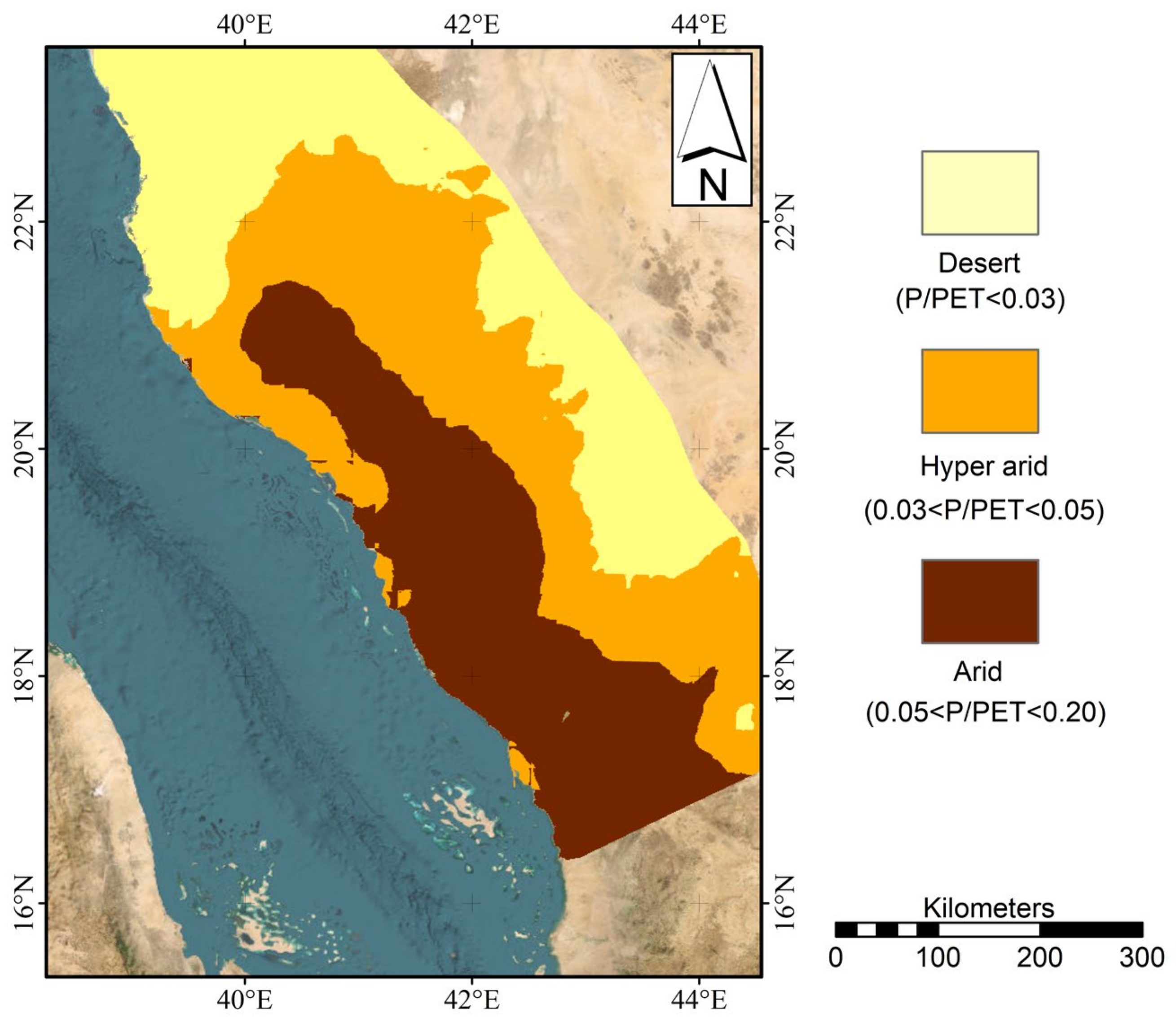
Figure 14 exhibits the spatial distribution of the average Aridity Index within the study area. The figure highlights that the majority of the study area falls within the hyper-arid classification, except the mountainous southern and southwestern regions, which are classified as arid zones.

5. Use Case

This section showcases a detailed example of how to deal with missing rainfall data in a network of stations for specific non-consecutive years (as indicated in Table 7) by using the findings outlined earlier.

The missing data for the years 2008 to 2010 can be directly retrieved from Figure S5, while the data for the years 2011 to 2013 can be acquired from Figure S6 in the Supplementary Materials, since these years fall after 2014. For the years 2015 to 2018, missing Material can be derived by employing ordinary Kriging interpolation with a J-Bessel semivariogram to generate geostatistical layers using the available data from adjacent stations, as demonstrated in Figure 15. The resulting missing data can be found in Table 8 after the filling process.

6. Summary and Conclusions

Rainfall depth and spatial distribution play a pivotal role in hydrological and water resources studies. While rain gauges are the conventional and most accurate data source, obtaining adequate records with accurate spatial distributions can be challenging, especially in regions with complex topography and security concerns, such as arid areas. In such contexts, satellite data and geostatistical interpolation techniques can be employed to estimate the spatial distribution between rain gauges and fill data gaps. However, the accuracy of satellite data in our study area was inadequate, underscoring the critical role of geostatistical interpolation in ensuring reliable rainfall spatial distribution.

This study focused on the southwest part of the Kingdom of Saudi Arabia, covering 123 rain gauges and spanning from 1966 to 2013. Throughout the study period, a total of 51 interpolation techniques were evaluated for total and maximum yearly precipitation records. Each year was assigned an optimal interpolation technique for maximum and total yearly precipitation data, determined by cross-validation to find the least centered Root Mean Square Error among the tested techniques. This optimal technique was then utilized to generate maximum and total yearly rainfall spatial distributions over the study area for each year from 1966 to 2013.

Similarly, interpolation techniques were chosen for mean annual values of the gap-filled data for total and maximum yearly rainfall, intended for years beyond 2013. For maximum yearly rainfall interpolation, ordinary Kriging with a J-Bessel semivariogram is recommended, while for total yearly rainfall, simple Kriging with a K-Bessel semivariogram is recommended.

In practical engineering applications within the study area, when utilizing rainfall time series is advised, the rasters provided in the Supplementary Materials can serve as valuable tools to address data gaps from 1966 to 2013. For data gaps extending beyond 2013, the use of KOJ and KSK techniques is recommended for interpolating maximum daily and total yearly rainfall values, respectively.

The average annual interpolated total rainfall depth and average annual potential evapotranspiration were utilized to develop the spatial distribution of the study area’s Aridity Index. Consequently, the study area was classified into three zones based on the Aridity Index scale: desert, hyper-arid, and arid zones.

A methodology was introduced, suggesting the incorporation of additional stations to enhance accuracy and reduce cross-validation errors. Intriguingly, the integration of another 23 stations resulted in a 21% improvement in the sum of the cross-validation error for maximum and total yearly precipitation. A practical use case clearly illustrates the proposed methodology, effectively showcasing its utility for engineering purposes.

Supplementary Materials

The following supporting information can be downloaded at: https://www.mdpi.com/article/10.3390/su151814028/s1, Figure S1: Distribution of maximum annual rainfall from 1966 to 1974, Figure S2: Distribution of maximum annual rainfall from 1965 to 1983, Figure S3: Distribution of maximum annual rainfall from 1984 to 1992, Figure S4: Distribution of maximum annual rainfall from 1993 to 2001, Figure S5: Distribution of maximum annual rainfall from 2002 to 2010, Figure S6: Distribution of maximum annual rainfall from 2011 to 2013, Figure S7: Distribution of total annual rainfall from 1966 to 1974; Figure S8: Distribution of total annual rainfall from 1965 to 1983, Figure S9: Distribution of total annual rainfall from 1984 to 1992, Figure S10: Distribution of total annual rainfall from 1993 to 2001, Figure S11: Distribution of total annual rainfall from 2002 to 2010, Figure S12: Distribution of total annual rainfall from 2011 to 2013, Figure S13: Total yearly rainfall cross-validation error for (A) existing rainfall stations, (B) with additional proposed stations (I), (C) with additional proposed stations (I) and (II), and 9D) with additional proposed stations (I), (II), and (III), Figure S14: Maximum daily rainfall cross-validation error for (A) existing rainfall stations, (B) with additional proposed stations (I), (C) with additional proposed stations (I) and (II), and (D) with additional proposed stations (I), (II), and (III).

Author Contributions

A.M.H.: Conceptualization, Data Collection, Data Analysis, Methodology, Visualization, Writing—Review and Editing. M.E.: Data Analysis, Methodology, Visualization, Writing—Review and Editing, Supervision. M.I.F.: Methodology, Visualization, Writing—Review and Editing. M.S.A.: Data Analysis, Writing—Review and Editing. B.T.E.: Data Collection, Methodology, Visualization, Writing—Original Draft. All authors have read and agreed to the published version of the manuscript.

Funding

This work was supported and funded by the Deanship of Scientific Research at Imam Mohammad Ibn Saud Islamic University (IMSIU) (grant number IMSIU-RG23109).

Institutional Review Board Statement

Not applicable.

Informed Consent Statement

Not applicable.

Data Availability Statement

Data will be made available on request.

Conflicts of Interest

The authors declare that they have no known competing financial interests or personal relationships that could have appeared to influence the work reported in this paper.

Appendix A. Spatial Interpolation Equations and Main Characteristics

Spatial interpolation is the estimation of missing measured parameters at specific locations over the study area by utilizing available data. In the current study, two approaches of spatial interpolation were used: (A) deterministic and (B) geostatistical. In the deterministic approach, the relation between points is presented in the form of a mathematical equation. On the other hand, the geostatistical approach is a probabilistic approach considering the spatial variance. Table A1 shows a summary of the advantages and disadvantages of interpolation techniques.

(A): Deterministic Approaches
(A.1.): Inverse Distance Weighting (IDW)

Inverse Distance Weighting is widely used due to its simplicity. Inverse Distance Weighting assigns weights to the surrounding measured data inversely proportional to each point separating distance. The power exponent (P) in the function varies between 0 and 6. With an increase in the power exponent, the weight of each point decreases faster with distance.

Z_{x} = \sum_{i = 1}^{N} λ_{i} Z_{i}

(A1)

λ_{i} = \frac{d_{x i}^{- P}}{\sum_{i = 1}^{N} d_{x i}^{- P}}

(A2)

where:

$Z_{x}$ : the predicted unknown value at point $(x)$ .
$λ_{i}$ : the weight value of the sampled point $(i)$ .
$Z_{i}$ : the value of the sampled point $(i)$ .
$d_{x i}$ : the distance between the sampled point $(i)$ and the predicted point $(x)$ .
$P$ : the power of decreasing weight with distance.

(A.2.): Global Polynomial Interpolation

The global polynomial is a multiple regression between all measured data over the study area. It starts from the first order up to the tenth.

Z_{(x_{i}, y_{i})} = β_{o} + β_{1} \cdot x_{i} + β_{2} \cdot y_{i} + ε (x_{i}, y_{i})

(A3)

Z_{(x_{i}, y_{i})} = β_{o} + β_{1} \cdot x_{i} + β_{2} \cdot y_{i} + β_{3} \cdot x_{i}^{2} + β_{4} \cdot y_{i}^{2} + β_{5} \cdot x_{i} \cdot y_{i} + β_{6} \cdot x_{i}^{3} + β_{7} \cdot y_{i}^{3} + β_{8} \cdot x_{i}^{2} \cdot y_{i} + β_{9} \cdot x_{i} \cdot y_{i}^{2} + ε (x_{i}, y_{i})

(A4)

where:

$Z_{(x_{i}, y_{i})}$ : location $(x_{i}, y_{i})$ value.
$ε (x_{i}, y_{i})$ : random error.
$β$ : parameter.

(A.3.): Local Polynomial Interpolation

Local Polynomial Interpolation has the same procedure as Global Polynomial Interpolation. Local Polynomial Interpolation is conducted over individual windows of the study area, not the whole area, as for Global Polynomial Interpolation.

(A.4.): Radial Basis Function

The Radial Basis Function generates an interpolated surface over the whole study area by utilizing one of the following five spline equations.

R e g u l a r i z e d s p l i n e f u n c t i o n — Ø (r) = l n {(σ \cdot \frac{r}{2})}^{2} + E_{1} {(σ \cdot r)}^{2} + C_{E}

(A5)

where:

$Ø (r)$ : Radial Basis Function.
$r$ : distance between the predicted point and each data location.
$E_{1} :$ exponential integer [82].
$C_{E} :$ Euler constant [82].

S p l i n e w i t h t e n s i o n f u n c t i o n — Ø (r) = l n (σ \cdot \frac{r}{2}) + K_{o} (σ \cdot \frac{r}{2}) + C_{E}

(A6)

where:

$K_{o} :$ modified Bessel function

M u l t i q u a d r i c f u n c t i o n — Ø (r) = {(r^{2} + σ^{2})}^{1 / 2}

(A7)

I n v e r s e m u l t i q u a d r i c f u n c t i o n — Ø (r) = {(r^{2} + σ^{2})}^{- 1 / 2}

(A8)

T h i n p l a t e s p l i n e f u n c t i o n — Ø (r) = {(σ \cdot r)}^{2} l n (σ \cdot r)

(A9)

(B): Geostatistical Approaches

The main difference between geostatistical and deterministic interpolation techniques is the consideration of the parameters’ spatial variability in the geostatistical approach. The observed variance with distance is transferred to a theoretical one that can be represented mathematically in the interpolation process. Equation (A10) illustrates the calculation of the semivariance. The variable (

γ

) is named semivariance because it calculates half of the variance, not the entire variance.

γ (h) = \frac{1}{2 N (h)} \sum_{i = 1}^{N (h)} {(Z (u_{i}) - Z (u_{i} + h))}^{2}

(A10)

where

Z (u_{i}) and Z (u_{i} + h)

are the values of the at the locations

(u_{i}) and (u_{i} + h)

, respectively.

Figure A1 shows a schematic diagram of a semivariogram. Several mathematical equations can be utilized to represent the theoretical semivariogram. In the current study, seven mathematical models were evaluated (Circular, Spherical, Exponential, Gaussian, K-Bessel, J-Bessel, and Stable).

Figure A1. Schematic semivariogram.

The geostatistical analysis estimates the missing values at location

(u_{o})

by assigning weights to the measured values, as shown in Equation (A11).

z^{*} (u_{o}) = \sum_{i = 1}^{n} λ_{i} z (u_{i})

(A11)

where:

$z^{*} (u_{o})$ : an estimate of the variable of interest at the location $(u_{o})$ .
$z (u_{i}) :$ the measured value of the variable of interest at the location $(u_{i})$ .
$λ_{i} :$ the Kriging weight of $z (u_{i})$ .
$n$ : the total number of data locations.

Geostatistical prediction is subjected to two main constraints: (A) the unbiasedness as given in Equation (A12), and (B) minimization of the variance of the estimated value

(z^{*} (u_{o}))

, shown in Equation (A13).

E [z^{*} (u_{o}) - z^{*} (u_{o})] = 0 \Rightarrow \sum_{i = 1}^{n} λ_{i} = 1

(A12)

E {[z^{*} (u_{o}) - z (u_{o})]}^{2} = \sum_{i = 1}^{n} \sum_{j = 1}^{n} λ_{i} λ_{j} γ_{i j} - 2 \sum_{i = 1}^{n} λ_{i} γ_{i o} + C (o)

(A13)

(B.1.): Simple Kriging

In simple Kriging, the stationary random parameter mean

(μ)

is assumed constant and known before Kriging. The model prediction parameters are given by Equation (A14).

(\begin{matrix} \begin{matrix} γ_{11} & γ_{12} & γ_{13} \\ γ_{21} & γ_{22} & γ_{23} \\ γ_{31} & γ_{32} & γ_{33} \end{matrix} & \dots & \begin{matrix} γ_{1 n} \\ γ_{2 n} \\ γ_{23 n} \end{matrix} \\ ⋮ & ⋱ & ⋮ \\ \begin{matrix} γ_{n 1} & γ_{n 2} & γ_{n 3} \end{matrix} & \dots & γ_{n n} \end{matrix}) (\begin{matrix} λ_{1} \\ λ_{2} \\ \begin{matrix} λ_{3} \\ ⋮ \\ λ_{n} \end{matrix} \end{matrix}) = (\begin{matrix} γ_{01} \\ γ_{02} \\ \begin{matrix} γ_{03} \\ ⋮ \\ γ_{0 n} \end{matrix} \end{matrix})

(A14)

(B.2.): Ordinary Kriging

In ordinary Kriging, the stationary random parameter mean

(μ)

is assumed constant and known before Kriging. The prediction parameters are given by Equation (A15)

(\begin{matrix} γ_{11} & γ_{12} & γ_{13} & \dots & γ_{1 n} & 1 \\ γ_{21} & γ_{22} & γ_{23} & \dots & γ_{2 n} & 1 \\ γ_{31} & γ_{32} & γ_{33} & \dots & γ_{3 n} & 1 \\ ⋮ & ⋮ & ⋮ & ⋱ & ⋮ & 1 \\ γ_{n 1} & γ_{n 2} & γ_{n 3} & \dots & γ_{n n} & 1 \\ 1 & 1 & 1 & \dots & 1 & 0 \end{matrix}) (\begin{matrix} λ_{1} \\ λ_{2} \\ λ_{3} \\ \begin{matrix} λ_{n} \\ m \end{matrix} \end{matrix}) = (\begin{matrix} γ_{01} \\ γ_{02} \\ \begin{matrix} γ_{03} \\ γ_{0 n} \\ 1 \end{matrix} \end{matrix})

(A15)

where:

$m :$ the mean value of the stationary variable.

(B.3.): Universal Kriging

If the concerned parameters exhibit a trend leading to nonstationary mean behavior, the sampling domain can be limited [83]. Kriging with a trend is another name of universal Kriging. In universal Kriging, another set of unbiasedness conditions is required. The prediction parameters are given by Equation (A16).

(\begin{matrix} γ_{11} & γ_{12} & γ_{13} & \dots & γ_{1 n} & 1 & {f_{1}}^{1} & {f_{1}}^{2} & \dots & {f_{1}}^{L} \\ γ_{21} & γ_{22} & γ_{23} & \dots & γ_{2 n} & 1 & {f_{2}}^{1} & {f_{2}}^{2} & \dots & {f_{2}}^{L} \\ γ_{31} & γ_{32} & γ_{33} & \dots & γ_{3 n} & 1 & {f_{3}}^{1} & {f_{3}}^{1} & \dots & {f_{3}}^{L} \\ ⋮ & ⋮ & ⋮ & ⋱ & ⋮ & ⋮ & ⋮ & ⋮ & ⋱ & ⋮ \\ γ_{n 1} & γ_{n 2} & γ_{n 3} & \dots & γ_{n n} & 1 & {f_{n}}^{1} & {f_{n}}^{2} & \dots & {f_{n}}^{L} \\ 1 & 1 & 1 & \dots & 1 & 0 & 0 & 0 & 0 & 0 \\ {f_{1}}^{1} & {f_{2}}^{1} & {f_{3}}^{1} & \dots & {f_{n}}^{1} & 0 & 0 & 0 & 0 & 0 \\ {f_{1}}^{2} & {f_{2}}^{2} & {f_{3}}^{2} & \dots & {f_{n}}^{2} & 0 & 0 & 0 & 0 & 0 \\ ⋮ & ⋮ & ⋮ & ⋱ & ⋮ & 0 & 0 & 0 & 0 & 0 \\ {f_{1}}^{L} & {f_{2}}^{L} & {f_{3}}^{L} & \dots & {f_{n}}^{2} & 0 & 0 & 0 & 0 & 0 \end{matrix}) (\begin{matrix} λ_{1} \\ λ_{2} \\ λ_{3} \\ ⋮ \\ µ_{0} \\ µ_{1} \\ µ_{2} \\ µ_{3} \\ ⋮ \\ µ_{L} \end{matrix}) = (\begin{matrix} γ_{01} \\ γ_{02} \\ \begin{matrix} γ_{03} \\ γ_{0 n} \\ {f_{1}}^{0} \\ {f_{2}}^{0} \\ {f_{3}}^{0} \\ ⋮ \\ {f_{L}}^{0} \end{matrix} \end{matrix})

(A16)

where:

$L$ : the number of unbiasedness conditions.
$f_{P}^{L}$ : the P^th basis function.

(B.4.): Cokriging

Cokriging is used when there are several variables. In the current study, we have two variables: (A) the rainfall depth and (B) the elevation of the rain gauges. The mathematical formulas of Cokriging can be found in [84,85,86,87,88].

(B.5.): Empirical Bayesian Kriging

There is a shortage in the literature regarding detailed descriptions of Empirical Bayesian Kriging (EBK). Most of the available documents focus computer package use [68,89].

Table A1. Summary of advantages and disadvantages of interpolation techniques.

Interpolation Technique	Advantages	Disadvantages
Inverse Distance Weighting	Simple and easy to apply. Fast computing time.	Generates “Bulls Eyes” at measurement locations. Sensitive to the selection of power factor. Sensitive to outliers.
Global Polynomial Interpolation	Simple and easy to apply. Fast computing time. Provides a smooth interpolated surface over the whole study area.	Does not capture local trends. Sensitive to the polynomial degree. Large influence of the edge points.
Local Polynomial Interpolation	Flexibility (allows the selection between several polynomial degrees). Captures local trends. Can handle complex patterns.	High computational demand. Sensitive to the polynomial degree. May generate discontinuity at local region edges
Radial Basis Function	Flexibility (allows the selection between five basis functions). Captures local trends. Can capture complex spatial patterns.	High computational demand. Sensitive to basis function selection.
Kriging	Provides Best Linear Unbiased Prediction (BLUP). Several types of Kriging provide flexibility to deal with stationary and non-stationary variables.	Requires preparing a variogram before starting the computation. Sensitive to model assumption. Computationally demanding.
Cokriging	Provide Best Linear Unbiased Prediction (BLUP). Several types of kriging provide flexibility to deal with stationary and non-stationary variables. Can handle more than one variable simultaneously. Incorporation of auxiliary variables can improve prediction accuracy.	Requires preparing a variogram before starting the computation. Sensitive to model assumption. The highest computational demand approach.
Empirical Bayesian Kriging	Automated variogram generation.	Limited theoretical justificationOutliers sensitivity

References

Gaur, M.K.; Squires, V.R. Geographic Extent and Characteristics of the World’s Arid Zones and Their Peoples. In Climate Variability Impacts on Land Use and Livelihoods in Drylands; Gaur, M.K., Squires, V.R., Eds.; Springer International Publishing: Cham, Switzerland, 2018; pp. 3–20. ISBN 978-3-319-56681-8. [Google Scholar]
Khan, M.Y.A.; ElKashouty, M.; Subyani, A.M.; Tian, F.; Gusti, W. GIS and RS intelligence in delineating the groundwater potential zones in Arid Regions: A case study of southern Aseer, southwestern Saudi Arabia. Appl. Water Sci. 2022, 12, 3. [Google Scholar] [CrossRef]
Wang, R.; Chen, J.; Chen, X.; Wang, Y. Variability of precipitation extremes and dryness/wetness over the southeast coastal region of China, 1960–2014. Int. J. Climatol. 2017, 37, 4656–4669. [Google Scholar] [CrossRef]
Mallick, J.; Talukdar, S.; Alsubih, M.; Salam, R.; Ahmed, M.; Ben Kahla, N.; Shamimuzzaman, M. Analysing the trend of rainfall in Asir region of Saudi Arabia using the family of Mann-Kendall tests, innovative trend analysis, and detrended fluctuation analysis. Theor. Appl. Climatol. 2021, 143, 823–841. [Google Scholar] [CrossRef]
Kharrou, M.H.; Le Page, M.; Chehbouni, A.; Simonneaux, V.; Er-Raki, S.; Jarlan, L.; Ouzine, L.; Khabba, S.; Chehbouni, G. Assessment of Equity and Adequacy of Water Delivery in Irrigation Systems Using Remote Sensing-Based Indicators in Semi-Arid Region, Morocco. Water Resour. Manag. 2013, 27, 4697–4714. [Google Scholar] [CrossRef]
Brunner, M.I.; Slater, L.; Tallaksen, L.M.; Clark, M. Challenges in modeling and predicting floods and droughts: A review. Wiley Interdiscip. Rev. Water 2021, 8, e1520. [Google Scholar] [CrossRef]
Hao, Z.; Singh, V.P.; Xia, Y. Seasonal Drought Prediction: Advances, Challenges, and Future Prospects. Rev. Geophys. 2018, 56, 108–141. [Google Scholar] [CrossRef]
Pachauri, K.; Meyer, L. Climate Change 2014 Synthesis Report; IPCC: Geneva, Switzerland, 2000; ISBN 9789291691432. [Google Scholar]
Al Mamoon, A.; Rahman, A. Rainfall in Qatar: Is it changing? Nat. Hazards 2017, 85, 453–470. [Google Scholar] [CrossRef]
Donat, M.G.; Lowry, A.L.; Alexander, L.V.; O’Gorman, P.A.; Maher, N. More extreme precipitation in the worldâ €^TM s dry and wet regions. Nat. Clim. Chang. 2016, 6, 508–513. [Google Scholar] [CrossRef]
Gebregiorgis, A.S.; Hossain, F. Understanding the dependence of satellite rainfall uncertainty on topography and climate for hydrologic model simulation. IEEE Trans. Geosci. Remote Sens. 2013, 51, 704–718. [Google Scholar] [CrossRef]
Arora, M.; Singh, P.; Goel, N.K.; Singh, R.D. Spatial distribution and seasonal variability of rainfall in a mountainous basin in the Himalayan region. Water Resour. Manag. 2006, 20, 489–508. [Google Scholar] [CrossRef]
Buytaert, W.; Celleri, R.; Willems, P.; De Bièvre, B.; Wyseure, G. Spatial and temporal rainfall variability in mountainous areas: A case study from the south Ecuadorian Andes. J. Hydrol. 2006, 329, 413–421. [Google Scholar] [CrossRef]
Hu, Q.; Li, Z.; Wang, L.; Huang, Y.; Wang, Y.; Li, L. Rainfall spatial estimations: A review from spatial interpolation to multi-source data merging. Water 2019, 11, 579. [Google Scholar] [CrossRef]
Kundzewicz, Z.W. Climate change impacts on the hydrological cycle. Ecohydrol. Hydrobiol. 2008, 8, 195–203. [Google Scholar] [CrossRef]
Lorenz, C.; Kunstmann, H. The hydrological cycle in three state-of-the-art reanalyses: Intercomparison and performance analysis. J. Hydrometeorol. 2012, 13, 1397–1420. [Google Scholar] [CrossRef]
Besha, K.Z.; Demissie, T.A.; Feyessa, F.F. Comparative analysis of long-term precipitation trends and its implication in the Modjo catchment, central Ethiopia. J. Water Clim. Chang. 2022, 13, 3883–3905. [Google Scholar] [CrossRef]
Kessabi, R.; Hanchane, M.; Caloiero, T.; Pellicone, G.; Addou, R.; Krakauer, N.Y. Analyzing Spatial Trends of Precipitation Using Gridded Data in the Fez-Meknes Region, Morocco. Hydrology 2023, 10, 37. [Google Scholar] [CrossRef]
Haggag, M.; Elsayed, A.A.; Awadallah, A.G. Evaluation of rain gauge network in arid regions using geostatistical approach: Case study in northern Oman. Arab. J. Geosci. 2016, 9, 552. [Google Scholar] [CrossRef]
Noori, M.J.; Hassan, H.H.; Mustafa, Y.T. Spatial Estimation of Rainfall Distribution and Its Classification in Duhok Governorate Using GIS. J. Water Resour. Prot. 2014, 6, 75–82. [Google Scholar] [CrossRef]
Keblouti, M.; Ouerdachi, L.; Boutaghane, H. Spatial interpolation of annual precipitation in Annaba- Algeria-Comparison and evaluation of methods. Energy Procedia 2012, 18, 468–475. [Google Scholar] [CrossRef]
Radi, N.F.A.; Zakaria, R.; Azman, M.A.Z. Estimation of missing rainfall data using spatial interpolation and imputation methods. AIP Conf. Proc. 2015, 1643, 42–48. [Google Scholar] [CrossRef]
WMO. Volume I: Hydrology—From Measurement to Hydrological Information; WMO: Geneva, Switzerland, 2008; Volume I, ISBN 9789263101686. [Google Scholar]
De Moraes Cordeiro, A.L.; Blanco, C.J.C. Assessment of satellite products for filling rainfall data gaps in the Amazon region. Nat. Resour. Model. 2021, 34, 12298. [Google Scholar] [CrossRef]
Al-Areeq, A.M.; Al-Zahrani, M.A.; Sharif, H.O. Assessment of the performance of satellite rainfall products over Makkah watershed using a physically based hydrologic model. Appl. Water Sci. 2022, 12, 246. [Google Scholar] [CrossRef]
Hobouchian, M.P.; Salio, P.; García Skabar, Y.; Vila, D.; Garreaud, R. Assessment of satellite precipitation estimates over the slopes of the subtropical Andes. Atmos. Res. 2017, 190, 43–54. [Google Scholar] [CrossRef]
Hsu, K.L.; Gao, X.; Sorooshian, S.; Gupta, H.V. Precipitation estimation from remotely sensed information using artificial neural networks. J. Appl. Meteorol. 1997, 36, 1176–1190. [Google Scholar] [CrossRef]
Portuguez-maurtua, M.; Arumi, J.L.; Lagos, O.; Stehr, A.; Arquiñigo, N.M. Filling Gaps in Daily Precipitation Series Using Regression and Machine Learning in Inter-Andean Watersheds. Water 2022, 14, 1799. [Google Scholar] [CrossRef]
Helmi, A.M.; Abdelhamed, M.S. Evaluation of CMORPH, PERSIANN-CDR, CHIRPS V2.0, TMPA 3B42 V7, and GPM IMERG V6 Satellite Precipitation Datasets in Arabian Arid Regions. Water 2023, 15, 92. [Google Scholar] [CrossRef]
Zhou, F.; Guo, H.C.; Ho, Y.S.; Wu, C.Z. Scientometric analysis of geostatistics using multivariate methods. Scientometrics 2007, 73, 265–279. [Google Scholar] [CrossRef]
Li, J.; Heap, A.D. A review of comparative studies of spatial interpolation methods in environmental sciences: Performance and impact factors. Ecol. Inform. 2011, 6, 228–241. [Google Scholar] [CrossRef]
Li, J.; Heap, A.D. Spatial interpolation methods applied in the environmental sciences: A review. Environ. Model. Softw. 2014, 53, 173–189. [Google Scholar] [CrossRef]
Wagner, P.D.; Fiener, P.; Wilken, F.; Kumar, S.; Schneider, K. Comparison and evaluation of spatial interpolation schemes for daily rainfall in data scarce regions. J. Hydrol. 2012, 464–465, 388–400. [Google Scholar] [CrossRef]
Sahu, B.; Ghosh, A.K. Seema Deterministic and geostatistical models for predicting soil organic carbon in a 60 ha farm on Inceptisol in Varanasi, India. Geoderma Reg. 2021, 26, e00413. [Google Scholar] [CrossRef]
Zhang, Y.; Hou, J.; Huang, C. Integration of Satellite-Derived and Ground-Based Soil Moisture Observations for a Precipitation Product over the Upper Heihe River Basin, China. Remote Sens. 2022, 14, 5355. [Google Scholar] [CrossRef]
Brindha, K.; Taie Semiromi, M.; Boumaiza, L.; Mukherjee, S. Comparing Deterministic and Stochastic Methods in Geospatial Analysis of Groundwater Fluoride Concentration. Water 2023, 15, 1707. [Google Scholar] [CrossRef]
Li, J.; Heap, A.D. A Review of Spatial Interpolation Methods for Environmental Scientists; Geoscience Australia: Canberra, Australia, 2008; Volume 68, ISBN 978 1 921498 30 5. [Google Scholar]
Chinchorkar, S.; Sayyad, F.; Patel, G.; Chinchorkar, S.S.; Patel, G.R.; Sayyad, F.G. Development of monsoon model for long range forecast rainfall explored for Anand (Gujarat-India). Int. J. Water Resour. Environ. Eng. 2012, 4, 322–326. [Google Scholar] [CrossRef]
Lu, B.; Charlton, M.; Harris, P.; Fotheringham, A.S. Geographically weighted regression with a non-Euclidean distance metric: A case study using hedonic house price data. Int. J. Geogr. Inf. Sci. 2014, 28, 660–681. [Google Scholar] [CrossRef]
Naoum, S.; Tsanis, I.K. A multiple linear regression GIS module using spatial variables to model orographic rainfall. J. Hydroinformatics 2004, 6, 39–56. [Google Scholar] [CrossRef]
Yeh, H.C.; Chen, Y.C.; Wei, C.; Chen, R.H. Entropy and kriging approach to rainfall network design. Paddy Water Environ. 2011, 9, 343–355. [Google Scholar] [CrossRef]
Mair, A.; Fares, A. Comparison of Rainfall Interpolation Methods in a Mountainous Region of a Tropical Island. J. Hydrol. Eng. 2011, 16, 371–383. [Google Scholar] [CrossRef]
Getahun, Y.S. Spatial-Temporal Analysis of Climate Elements, Vegetation Characteristics, and Sea Surface Temperature Anomaly—A Case Study in Gojam, Ethiopia, Erasmus Mundus Program-European Union. Master’s Thesis, Universidade NOVA de Lisboa, Lisbon, Portugal, 2012. [Google Scholar]
Page, T.; Beven, K.J.; Hankin, B.; Chappell, N.A. Interpolation of rainfall observations during extreme rainfall events in complex mountainous terrain. Hydrol. Process. 2022, 36, 14758. [Google Scholar] [CrossRef]
Jacquin, A. Interpolation of daily precipitation in mountain catchments with limited data availability. In Proceedings of the EGU General Assembly Conference Abstracts; European Geosciences Union: Munich, Germany, 2014; p. 13973. [Google Scholar]
Yang, R.; Xing, B. A comparison of the performance of different interpolation methods in replicating rainfall magnitudes under different climatic conditions in chongqing province (China). Atmosphere 2021, 12, 1318. [Google Scholar] [CrossRef]
Ali, G.; Sajjad, M.; Kanwal, S.; Xiao, T.; Khalid, S.; Shoaib, F.; Gul, H.N. Spatial–temporal characterization of rainfall in Pakistan during the past half-century (1961–2020). Sci. Rep. 2021, 11, 6935. [Google Scholar] [CrossRef] [PubMed]
Yang, X.; Xie, X.; Liu, D.L.; Ji, F.; Wang, L. Spatial Interpolation of Daily Rainfall Data for Local Climate Impact Assessment over Greater Sydney Region. Adv. Meteorol. 2015, 2015, 563629. [Google Scholar] [CrossRef]
Amini, M.A.; Torkan, G.; Eslamian, S.; Zareian, M.J.; Adamowski, J.F. Analysis of deterministic and geostatistical interpolation techniques for mapping meteorological variables at large watershed scales. Acta Geophys. 2019, 67, 191–203. [Google Scholar] [CrossRef]
Delbari, M.; Afrasiab, P.; Jahani, S. Spatial interpolation of monthly and annual rainfall in northeast of Iran. Meteorol. Atmos. Phys. 2013, 122, 103–113. [Google Scholar] [CrossRef]
Gupta, A.; Kamble, T.; Machiwal, D. Comparison of ordinary and Bayesian kriging techniques in depicting rainfall variability in arid and semi-arid regions of north-west India. Environ. Earth Sci. 2017, 76, 512. [Google Scholar] [CrossRef]
Hasanean, H.; Almazroui, M. Rainfall: Features and variations over Saudi Arabia, a review. Climate 2015, 3, 578–626. [Google Scholar] [CrossRef]
OBG. The Report: Saudi Arabia; Oxford Business Group: Oxford, UK, 2019. [Google Scholar]
Chowdhury, S.; Al-Zahrani, M. Characterizing water resources and trends of sector wise water consumptions in Saudi Arabia. J. King Saud Univ. Eng. Sci. 2015, 27, 68–82. [Google Scholar] [CrossRef]
Al-Ahmadi, K.; Al-Ahmadi, S. Rainfall-altitude relationship in Saudi Arabia. Adv. Meteorol. 2013, 2013, 363029. [Google Scholar] [CrossRef]
Sultana, R.; Nasrollahi, N. Evaluation of remote sensing precipitation estimates over Saudi Arabia. J. Arid Environ. 2018, 151, 90–103. [Google Scholar] [CrossRef]
Al-Zahrani, M.; Husain, T. An algorithm for designing a precipitation network in the south-western region of Saudi Arabia. J. Hydrol. 1998, 205, 205–216. [Google Scholar] [CrossRef]
Hag-Elsafi, S.; El-Tayib, M. Spatial and statistical analysis of rainfall in the Kingdom of Saudi Arabia from 1979 to 2008. Weather 2016, 71, 262–266. [Google Scholar] [CrossRef]
Frenken, K. Irrigation in the Middle East Region in Figures, FAO Water Report—Aquastat Survey; FAO: Rome, Italy, 2009; Volume 34. [Google Scholar]
Almazroui, M. Calibration of TRMM rainfall climatology over Saudi Arabia during 1998–2009. Atmos. Res. 2011, 99, 400–414. [Google Scholar] [CrossRef]
Abdullah, M.A.; Almazroui, M. Climatological study of the southwestern region of Saudi Arabia. I. Rainfall analysis. Clim. Res. 1998, 9, 213–223. [Google Scholar] [CrossRef]
Subyani, A.M. Geostatistical study of annual and seasonal mean rainfall patterns in southwest Saudi Arabia/Distribution géostatistique de la pluie moyenne annuelle et saisonnière dans le Sud-Ouest de l’Arabie Saoudite. Hydrol. Sci. J. 2004, 49, 55137. [Google Scholar] [CrossRef]
World Bank. Making the Most of Scarcity Accountability for Better Water Management in the Middle East and North Africa; MENA Development Report; World Bank: Washington, DC, USA, 2007. [Google Scholar]
KSA-MWA. Hydrological Publications No. 98 Vol. 4 Years (1963–1980); Kingdom of Saudi Arabia, Minisrtry of Agriculture and Wate, Hydrology Division, Department of Water Resources and Development: Riyadh, Saudi Arabia, 1980. [Google Scholar]
Igaz, D.; Šinka, K.; Varga, P.; Vrbičanová, G.; Aydın, E.; Tárník, A. The evaluation of the accuracy of interpolation methods in crafting maps of physical and hydro-physical soil properties. Water 2021, 13, 212. [Google Scholar] [CrossRef]
Robinson, T.P.; Metternicht, G. Testing the performance of spatial interpolation techniques for mapping soil properties. Comput. Electron. Agric. 2006, 50, 97–108. [Google Scholar] [CrossRef]
Burrough, P.A.; McDonnell, R.A.; Lloyd, C.D. Principles of Geographical Information Systems; Oxford University Press: Oxford, UK, 2015; ISBN 0198742843. [Google Scholar]
Johnston, K.; Ver Hoef, J.M.; Krivoruchko, K.; Lucas, N. Using ArcGIS Geostatistical Analyst; ESRI: Redlands, CA, USA, 2001; ISBN 1589480066. [Google Scholar]
Bhunia, G.S.; Shit, P.K.; Maiti, R. Comparison of GIS-based interpolation methods for spatial distribution of soil organic carbon (SOC). J. Saudi Soc. Agric. Sci. 2018, 17, 114–126. [Google Scholar] [CrossRef]
Krige, D.G. A statistical approach to some basic mine valuation problems on the Witwatersrand. J. S. Afr. Inst. Min. Metall. 1951, 52, 119–139. [Google Scholar]
Adhikary, S.K.; Muttil, N.; Yilmaz, A.G. Cokriging for enhanced spatial interpolation of rainfall in two Australian catchments. Hydrol. Process. 2017, 31, 2143–2161. [Google Scholar] [CrossRef]
Liu, D.; Zhao, Q.; Fu, D.; Guo, S.; Liu, P.; Zeng, Y. Comparison of spatial interpolation methods for the estimation of precipitation patterns at different time scales to improve the accuracy of discharge simulations. Hydrol. Res. 2020, 51, 583–601. [Google Scholar] [CrossRef]
Javari, M. Comparison of interpolation methods for modeling spatial variations of Precipitation in Iran. Int. J. Environ. Sci. Educ. 2016, 11, 349–358. [Google Scholar]
Mirzaei, R.; Sakizadeh, M. Comparison of interpolation methods for the estimation of groundwater contamination in Andimeshk-Shush Plain, Southwest of Iran. Environ. Sci. Pollut. Res. 2016, 23, 2758–2769. [Google Scholar] [CrossRef] [PubMed]
Samsonova, V.P.; Blagoveshchenskii, Y.N.; Meshalkina, Y.L. Use of empirical Bayesian kriging for revealing heterogeneities in the distribution of organic carbon on agricultural lands. Eurasian Soil Sci. 2017, 50, 305–311. [Google Scholar] [CrossRef]
Shih, S.F. Rainfall variation analysis and optimization of gaging systems. Water Resour. Res. 1982, 18, 1269–1277. [Google Scholar] [CrossRef]
Chen, Y.-C.; Wei, C.; Yeh, H.-C. Rainfall network design using kriging and entropy. Hydrol. Process. 2008, 22, 340–346. [Google Scholar] [CrossRef]
Middleton, N.; Thomas, D. World Atlas of Desertification; United Nations Digital Library: Geneva, Switzerland, 1992; Volume ix, 69p. [Google Scholar]
Spinoni, J.; Vogt, J.; Naumann, G.; Carrao, H.; Barbosa, P. Towards identifying areas at climatological risk of desertification using the Köppen-Geiger classification and FAO aridity index. Int. J. Climatol. 2015, 35, 2210–2222. [Google Scholar] [CrossRef]
FAO. WaPOR Database Methodology, Version 2 Release, April 2020; FAO: Rome, Italy, 2020; ISBN 978-92-5-132981-8. [Google Scholar]
WaPOR WaPOR Portal. Available online: https://wapor.apps.fao.org/home/WAPOR_2/1 (accessed on 7 September 2023).
Abramowitz, M.; Stegun, I.A. Handbook of Mathematical Functions; Department of Commerce—United States of America: Dover, NY, USA, 1975. [Google Scholar]
Rojimol, J. Development of Optimal Geostatistical Model for Geotechnical Applications; Indian Institute of Technology Hyderabad: Sangareddy, India, 2013. [Google Scholar]
Journel, A.G.; Huijbregts, C. Mining Geostatistics; Academic Press: London, UK; New York, NY, USA, 1978; ISBN 0123910501. [Google Scholar]
Isaaks, E.H.; Srivastava, R.M. An Introduction to Applied Geostatistics; Oxford University Press: Oxford, UK, 1990; ISBN 978-0195050134. [Google Scholar]
Cressie, N. Fitting variogram models by weighted least squares. J. Int. Assoc. Math. Geol. 1985, 17, 563–586. [Google Scholar] [CrossRef]
Gooverts, P. Geostatistics for Natural Resources Evaluation; Oxford University Press: New York, NY, USA, 1997; ISBN 0-19-511538-4. [Google Scholar]
Chile, J.-P.; Delfiner, P. Geostatistics-Modeling Spatial Uncertainty, 2nd ed.; John Wiley & Sons, Inc.: Hoboken, NJ, USA, 2012; ISBN 978-0-470-18315-1. [Google Scholar]
Krivoruchko, K.; Gribov, A. Evaluation of empirical Bayesian kriging. Spat. Stat. 2019, 32, 100368. [Google Scholar] [CrossRef]

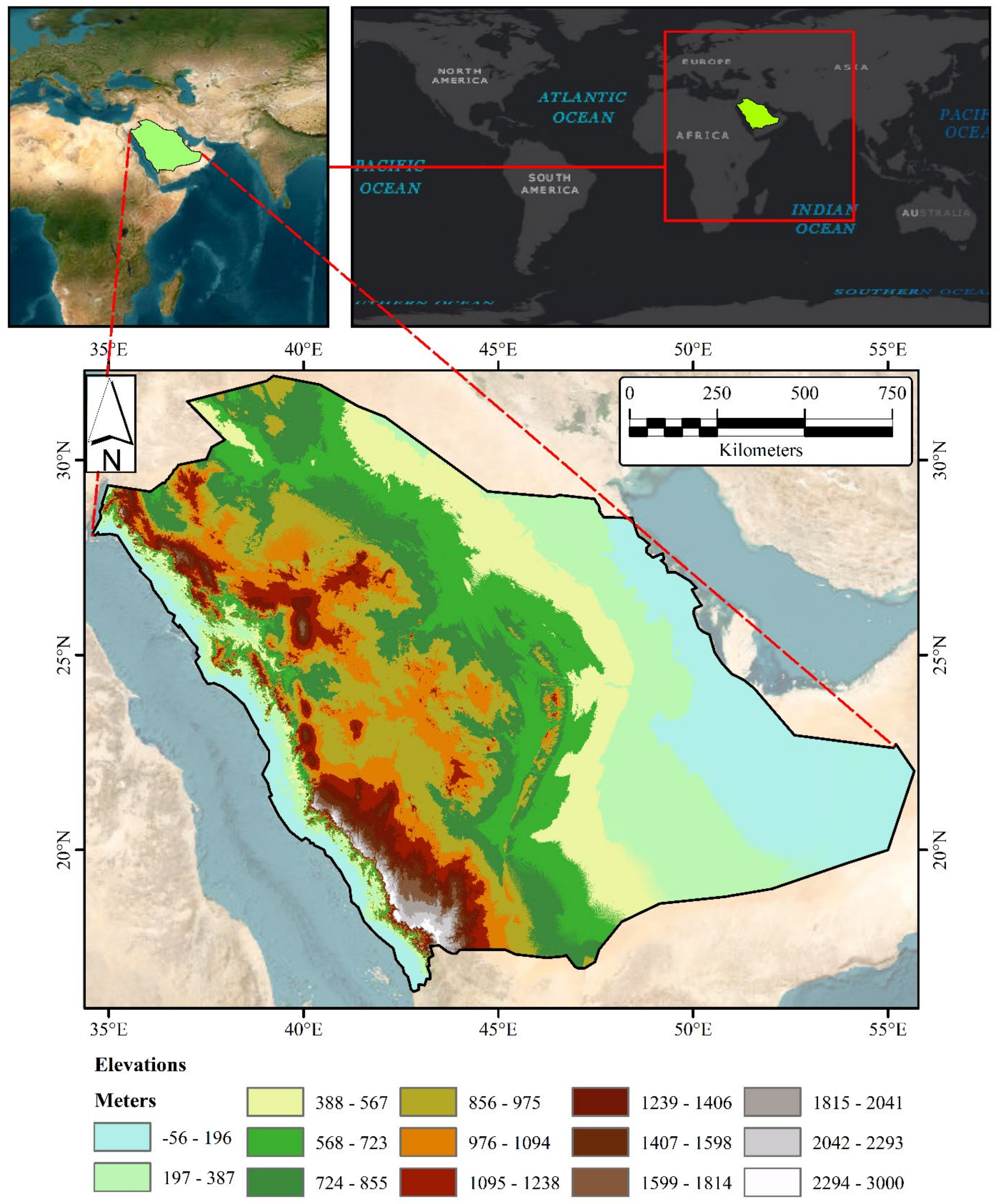
Figure 1. The KSA’s location and topography.

Figure 2. Average annual rainfall over the KSA, adopted from Helmi and Abdelhamed (2023) [29].

Figure 3. (A) The collected 128 rainfall gauges’ locations, (B) types of available rainfall gauges, (C) the selected rainfall gauges for the current study, and (D) elevations of the selected rain gauges.

Figure 4. Temporal variation in available rain gauge data in the study area.

Figure 5. Taylor diagram depicting total rainfall interpolation models for the year 1998.

Figure 6. Spatial distribution of total annual rainfall depth for the year 1999 (generated by CKSG geostatistical interpolation).

Figure 7. Spatial distribution of maximum daily rainfall for the year 1999 (generated by CKOC geostatistical interpolation).

Figure 8. The spatial distribution of the maximum and total yearly precipitation (mm).

Figure 9. Cross-validation error summation for total yearly and maximum daily rainfall for (A) existing rainfall stations, (B) with additional proposed stations (I), (C) with additional proposed stations (I) and (II), and (D) with additional proposed stations (I), (II), and (III).

Figure 10. Proposed additional stations.

Figure 11. Proposed methodology to select the location of additional stations.

Figure 12. Effect of increasing the number of rain gauge stations on the average CVE.

Figure 13. Time-averaged annual reference evapotranspiration.

Figure 14. Aridity classification in the study area.

Figure 15. Geostatistical surfaces for the years from 2015 to 2018.

Table 2. Characteristics of the selected rain gauges.

Gauge	Long (WGS 84)	Lat (WGS84)	Altitude (m)	Mean Max. Rainfall (mm)	Mean Total Rainfall (mm)	Gauge	Long (WGS 84)	Lat (WGS 84)	Altitude (m)	Mean Max. Rainfall (mm)	Mean Total Rainfall (mm)
A004	43.10	18.17	2280	31.9	97.9	J141	39.92	22.50	661	49.7	96.4
A005	42.48	18.20	2186	57.3	282.8	J204	40.20	21.35	685	39.7	154.0
A006	42.60	18.25	2121	40.3	238.5	J205	40.22	21.35	750	46.3	171.0
A007	42.15	19.10	2376	61.8	344.4	J214	39.98	21.98	641	33.5	97.0
A103	42.78	18.10	2224	39.5	237.9	J219	39.43	22.20	192	22.2	38.4
A104	43.37	17.93	2281	32.1	127.2	J220	39.82	22.37	473	23.4	62.2
A105	43.18	18.23	2206	23.9	70.1	J221	39.35	21.92	88	27.5	45.0
A106	42.48	18.27	2356	38.5	253.2	J239	39.68	21.97	269	23.9	64.1
A107	42.57	18.60	2016	31.9	109.8	N001	44.23	17.55	1278	19.8	44.5
A108	42.38	18.52	2516	26.4	85.0	N103	43.63	17.68	2191	34.2	145.9
A110	42.98	18.68	1802	33.9	98.3	N203	43.62	17.67	2036	26.9	94.3
A112	42.57	18.37	2096	36.2	112.4	SA001	42.95	17.05	169	36.4	203.0
A113	42.68	18.63	1840	17.5	69.3	SA002	42.62	17.17	32	28.2	80.2
A117	42.27	18.62	2489	38.2	181.7	SA003	41.88	19.00	355	37.5	202.7
A118	42.37	18.25	2197	56.7	333.7	SA004	41.40	18.73	41	27.4	61.2
A120	42.17	18.88	2308	56.0	213.9	SA005	41.88	19.56	2263	27.2	172.5
A121	42.75	18.03	2269	44.5	292.7	SA101	42.83	16.97	68	41.6	173.0
A123	42.87	18.32	2039	34.3	128.9	SA102	42.23	17.70	51	30.1	65.2
A124	42.33	18.42	2577	41.0	185.0	SA104	43.08	17.04	574	50.3	403.9
A126	43.22	18.53	1850	12.9	26.5	SA105	41.97	18.93	458	48.6	364.1
A127	42.25	18.78	2531	48.3	247.3	SA106	42.53	17.37	73	37.2	137.5
A128	42.70	18.47	1927	16.5	60.2	SA107	42.78	17.12	78	44.6	170.0
A130	42.32	18.33	2470	36.1	216.5	SA108	41.92	18.33	533	41.8	255.8
A201	42.52	18.42	2083	25.9	103.0	SA110	43.13	17.27	1210	47.1	401.0
A206	42.25	18.68	2603	39.1	206.6	SA111	43.12	17.05	574	54.5	444.1
A213	42.83	18.17	2114	30.4	132.0	SA113	42.03	18.53	455	41.3	298.1
B001	41.29	20.18	1932	58.9	294.0	SA115	41.67	18.00	0	28.1	54.6
B004	42.60	20.02	1155	21.3	71.8	SA116	42.20	18.25	1421	49.0	321.7
B005	42.53	19.87	1202	18.6	73.6	SA120	41.83	19.43	611	46.2	243.5
B006	43.52	19.53	1090	21.8	48.9	SA122	41.83	19.12	377	31.1	208.6
B007	41.57	19.87	2047	52.6	269.3	SA125	42.45	17.13	7	25.8	72.5
B008	42.67	20.08	1139	24.3	80.1	SA126	42.88	17.45	559	45.9	502.3
B009	41.90	19.53	2279	46.0	272.6	SA129	42.90	17.17	163	49.9	313.7
B101	41.58	19.90	2040	50.8	224.9	SA132	42.78	17.02	61	29.5	127.0
B103	41.65	20.25	1571	20.0	51.5	SA135	43.23	16.80	287	43.7	330.6
B110	42.88	18.80	1742	22.4	73.2	SA136	43.13	16.68	159	45.6	251.7
B111	42.85	21.25	922	18.4	48.8	SA137	42.95	16.60	61	29.5	116.3
B114	42.23	20.02	1286	25.5	98.2	SA138	42.02	18.63	393	39.7	267.1
B208	42.73	19.02	1717	20.3	69.6	SA139	42.03	19.05	900	26.2	293.3
B216	41.98	19.47	2239	42.9	234.8	SA140	43.03	17.32	688	49.7	448.6
B217	41.93	19.75	1756	43.0	170.4	SA142	41.58	18.77	104	32.3	101.9
B219	42.80	19.33	1475	18.4	53.1	SA143	43.13	16.90	259	46.3	420.7
B220	42.04	19.20	1571	36.0	142.6	SA144	42.25	18.17	1013	46.9	366.6
J001	41.05	19.53	53	36.8	77.3	SA145	42.80	17.62	699	46.0	306.8
J002	39.34	22.16	72	18.3	33.3	SA147	41.47	19.03	115	30.9	66.3
J102	39.70	21.43	355	27.8	50.3	SA148	42.53	16.92	0	35.5	79.0
J106	39.33	22.15	66	18.8	35.8	SA204	42.60	17.57	188	43.3	160.2
J107	40.45	20.32	95	34.1	63.6	TA002	40.50	21.30	1590	33.0	148.2
J108	40.28	20.15	7	32.8	59.8	TA004	40.45	21.40	1553	28.6	119.4
J111	38.83	23.10	12	17.4	33.7	TA005	41.67	21.18	1148	14.0	49.4
J113	40.12	21.37	455	47.8	146.0	TA006	41.28	20.62	1389	52.6	117.9
J114	39.82	21.43	298	37.9	78.6	TA007	41.47	19.98	2256	48.6	194.0
J116	39.63	22.58	394	28.2	63.3	TA104	40.80	21.32	1394	31.4	97.3
J121	41.05	20.23	338	40.9	162.1	TA106	40.32	21.33	1888	44.8	185.5
J124	41.28	19.95	586	30.0	114.4	TA109	40.37	21.07	2145	45.4	269.6
J126	41.43	19.77	353	37.3	236.8	TA125	40.42	21.26	1713	29.7	51.7
J127	41.53	19.67	657	52.7	184.0	TA206	40.40	21.28	1675	35.7	165.8
J131	41.60	19.47	474	41.9	182.6	TA233	40.65	21.13	1691	48.5	205.6
J134	39.20	21.50	15	28.7	51.4	TA250	40.45	21.67	1241	22.7	91.2
J137	41.33	19.97	632	36.4	222.3	TA251	40.37	21.37	1822	30.1	120.1
J139	41.03	19.73	93	38.6	63.9	TA255	40.36	21.24	1730	34.1	118.5
J140	39.03	22.82	10	21.1	39.4

Table 3. Codes of the 51 interpolation techniques used in the current study.

Geostatistical Interpolation Techniques
Ordinary Kriging—Circular Variogram (KOC)	Ordinary Cokriging—Circular Variogram (CKOC)
Ordinary Kriging—Spherical Variogram (KOS)	Ordinary Cokriging—Spherical Variogram (CKOS)
Ordinary Kriging—Exponential Variogram (KOE)	Ordinary Cokriging—Exponential Variogram (CKOE)
Ordinary Kriging—Gaussian Variogram (KOG)	Ordinary Cokriging—Gaussian Variogram (CKOG)
Ordinary Kriging—K-Bessel Variogram (KOK)	Ordinary Cokriging—K-Bessel Variogram (CKOK)
Ordinary Kriging—J-Bessel Variogram (KOJ)	Ordinary Cokriging—J-Bessel Variogram (CKOJ)
Ordinary Kriging—Stable Variogram (KOT)	Ordinary Cokriging—Stable Variogram (CKOT)
Simple Kriging—Circular Variogram (KSC)	Simple Cokriging—Circular Variogram (CKSC)
Simple Kriging—Spherical Variogram (KSS)	Simple Cokriging—Spherical Variogram (CKSS)
Simple Kriging—Exponential Variogram (KSE)	Simple Cokriging—Exponential Variogram (CKSE)
Simple Kriging—Gaussian Variogram (KSG)	Simple Cokriging—Gaussian Variogram (CKSG)
Simple Kriging—K-Bessel Variogram (KSK)	Simple Cokriging—K-Bessel Variogram (CKSK)
Simple Kriging—J-Bessel Variogram (KSJ)	Simple Cokriging—J-Bessel Variogram (CKSJ)
Simple Kriging—Stable Variogram (KST)	Simple Cokriging—Stable Variogram (CKST)
Universal Kriging—Circular Variogram (KUC)	Universal Cokriging—Circular Variogram (CKUC)
Universal Kriging—Spherical Variogram (KUS)	Universal Cokriging—Spherical Variogram (CKUS)
Universal Kriging—Exponential Variogram (KUE)	Universal Cokriging—Exponential Variogram (CKUE)
Universal Kriging—Gaussian Variogram (KUG)	Universal Cokriging—Gaussian Variogram (CKUG)
Universal Kriging—K-Bessel Variogram (KUK)	Universal Cokriging—K-Bessel Variogram (CKUK)
Universal Kriging—J-Bessel Variogram (KUJ)	Universal Cokriging—J-Bessel Variogram (CKUJ)
Universal Kriging—Stable Variogram (KUT)	Universal Cokriging—Stable Variogram (CKUT)
Empirical Bayesian Kriging (EBK)
Deterministic interpolation techniques
Global Polynomial Interpolation (GPI)	Inverse Distance Weighting—P = 2 (IDWP2)
Local Polynomial Interpolation (LPI)	Inverse Distance Weighting—P = 3 (IDWP)
Radial Basis Function (RBF)	Inverse Distance Weighting—P = 4 (IDWP4)
Inverse Distance Weighting (P = 1) (IDWP1)	Inverse Distance Weighting—P = 5 (IDWP)

Table 4. Yearly selected interpolation techniques for maximum daily and total annual rainfall over the study area.

Year	Total Yearly	Maximum Daily	Year	Total Yearly	Maximum Daily
1966	KOJ	CKOK	1990	CKUK	CKOJ
1967	KUJ	KUJ	1991	CKSJ	KOJ
1968	KSJ	CKUC	1992	CKOJ	KSG
1969	LPI	CKOJ	1993	CKUJ	CKSK
1970	KSJ	KUJ	1994	CKOS	KOJ
1971	CKOC	CKOC	1995	CKOC	CKUC
1972	CKOC	KOJ	1996	CKSE	CKOG
1973	CKOJ	KOJ	1997	CKUT	CKOT
1974	KOJ	CKOC	1998	CKUK	CKOK
1975	CKOJ	CKUJ	1999	CKSG	CKOC
1976	CKOJ	LPI	2000	KSG	KOE
1977	CKOG	CKUC	2001	KOT	KSJ
1978	CKOJ	KUJ	2002	CKSC	CKOG
1979	CKOT	CKOS	2003	KUJ	CKSJ
1980	KOJ	CKOJ	2004	KOJ	CKOJ
1981	CKSG	CKSJ	2005	CKSC	GPI
1982	CKSG	CKUJ	2006	KOG	CKOK
1983	CKUC	KOJ	2007	KOG	IDWP1
1984	CKOC	CKSK	2008	CKSJ	CKSG
1985	CKOE	CKOK	2009	CKSE	KUJ
1986	CKOC	KUJ	2010	KSG	CKOC
1987	KOJ	CKSK	2011	KSJ	KST
1988	KUK	CKOC	2012	CKOS	CKUJ
1989	CKUE	LPI	2013	CKOJ	CKOC

Table 5. Study area areal average cross-validation error (%).

	Maximum Rainfall Error (%)	Total Rainfall Error (%)	Error Summation (%)
Existing stations	14.60%	27.08%	41.68%
Existing stations + Proposed stations (I)	12.71%	22.34%	35.05%
Existing stations + Proposed stations (I) and (II)	11.65%	20.95%	32.61%
Existing stations + Proposed stations (I), (II), and (III)	11.51%	20.79%	32.31%

Table 6. Aridity level classification.

Aridity Level	Aridity Index (AI)
Desert	AI < 0.03
Hyper arid	0.03 < AI < 0.05
Arid	0.05 < AI < 0.20
Semi-arid	0.20 < AI < 0.50
Dry	0.50 < AI < 0.65
Sub-humid	0.65 < AI < 0.75
Humid	AI > 0.75
Cold	PET ≤ 400 mm

Table 7. Maximum rainfall records with missing entries.

	J124	B001	J137	J126	TA007	J127	B007	B101
2008	23.0	32.0	missing	26.78991	26.0	missing	46.0	19.0
2009	34.0	63.0	missing	33.0	54.5	missing	42.5	25.0
2010	60.0	56.0	missing	41.0	168.0	missing	54.0	45.0
2011	28.0	82.5	missing	22.0	60.0	missing	44.0	27.0
2012	40.0	missing	missing	17.0	34.5	missing	62.0	56.0
2013	26.5	missing	missing	28.0	24.5	missing	54.0	40.0
2014	7.3	30.8	70.4	35.5	37.8	40.5	36.1	41.5
2015	6.5	89.0	51.3	51.5	missing	50.8	59.0	missing
2016	32.0	69.0	50.5	50.8	missing	50.5	26.0	52.0
2017	1.3	78.8	24.5	21.6	missing	45.3	26.2	15.0
2018	5.0	34.4	42.5	21.5	missing	40.5	35.8	34.5

Table 8. Interpolated filled data.

	J124	B001	J137	J126	TA007	J127	B007	B101
2008	23.0	32.0	27.2	26.8	26.0	28.2	46.0	19.0
2009	34.0	63.0	46.4	33.0	54.5	51.4	42.5	25.0
2010	60.0	56.0	46.4	41.0	168.0	42.6	54.0	45.0
2011	28.0	82.5	30.4	22.0	60.0	22.9	44.0	27.0
2012	40.0	19.4	26.8	17.0	34.5	32.4	62.0	56.0
2013	26.5	30.0	30.9	28.0	24.5	32.5	54.0	40.0
2014	7.3	30.8	70.4	35.5	37.8	40.5	36.1	41.5
2015	6.5	89.0	51.3	51.5	50.4	50.8	59.0	52.9
2016	32.0	69.0	50.5	50.8	47.2	50.5	26.0	52.0
2017	16.0	78.8	24.5	21.6	24.4	45.3	26.2	15.0
2018	5.0	34.4	42.5	21.5	30.6	40.5	35.8	34.5

Disclaimer/Publisher’s Note: The statements, opinions and data contained in all publications are solely those of the individual author(s) and contributor(s) and not of MDPI and/or the editor(s). MDPI and/or the editor(s) disclaim responsibility for any injury to people or property resulting from any ideas, methods, instructions or products referred to in the content.

© 2023 by the authors. Licensee MDPI, Basel, Switzerland. This article is an open access article distributed under the terms and conditions of the Creative Commons Attribution (CC BY) license (https://creativecommons.org/licenses/by/4.0/).

Share and Cite

MDPI and ACS Style

Helmi, A.M.; Elgamal, M.; Farouk, M.I.; Abdelhamed, M.S.; Essawy, B.T. Evaluation of Geospatial Interpolation Techniques for Enhancing Spatiotemporal Rainfall Distribution and Filling Data Gaps in Asir Region, Saudi Arabia. Sustainability 2023, 15, 14028. https://doi.org/10.3390/su151814028

AMA Style

Helmi AM, Elgamal M, Farouk MI, Abdelhamed MS, Essawy BT. Evaluation of Geospatial Interpolation Techniques for Enhancing Spatiotemporal Rainfall Distribution and Filling Data Gaps in Asir Region, Saudi Arabia. Sustainability. 2023; 15(18):14028. https://doi.org/10.3390/su151814028

Chicago/Turabian Style

Helmi, Ahmed M., Mohamed Elgamal, Mohamed I. Farouk, Mohamed S. Abdelhamed, and Bakinam T. Essawy. 2023. "Evaluation of Geospatial Interpolation Techniques for Enhancing Spatiotemporal Rainfall Distribution and Filling Data Gaps in Asir Region, Saudi Arabia" Sustainability 15, no. 18: 14028. https://doi.org/10.3390/su151814028

Note that from the first issue of 2016, this journal uses article numbers instead of page numbers. See further details here.

Article Menu

Evaluation of Geospatial Interpolation Techniques for Enhancing Spatiotemporal Rainfall Distribution and Filling Data Gaps in Asir Region, Saudi Arabia

Abstract

1. Introduction

2. The Study Area

3. Materials and Methods

3.1. Rain Gauges

3.2. Interpolation Techniques

3.2.1. Deterministic Techniques

3.2.2. Geostatistical Techniques

4. Results and Discussion

5. Use Case

6. Summary and Conclusions

Supplementary Materials

Author Contributions

Funding

Institutional Review Board Statement

Informed Consent Statement

Data Availability Statement

Conflicts of Interest

Appendix A. Spatial Interpolation Equations and Main Characteristics

References

Share and Cite

Article Metrics

Article Access Statistics

Further Information

Guidelines

MDPI Initiatives

Follow MDPI