Spatiotemporal Variation and Future Predictions of Soil Salinization in the Werigan–Kuqa River Delta Oasis of China

Abstract

Soil salinization is a serious global issue; by 2050, without intervention, 50% of the cultivated land area will be affected by salinization. Therefore, estimating and predicting future soil salinity is crucial for preventing soil salinization and investigating potential arable land resources. In this study, several machine learning methods (random forest (RF), Light Gradient Boosting Machine (LightGBM), Gradient Boosting Decision Tree (GBDT), and eXtreme Gradient Boosting (XGBoost)) were used to estimate the soil salinity in the Werigan–Kuqa River Delta Oasis region of China from 2001 to 2021. The cellular automata (CA)–Markov model was used to predict soil salinity types from 2020 to 2050. The LightGBM method exhibited the highest accuracy, and the overall prediction accuracy of the methods had the following order: LightGBM > RF > GBRT > XGBoost. Moderately saline, severely saline, and saline soils were dominant in the east and south of the research area, while non-saline and mildly saline soils were widely distributed in the inner oasis area. A marked decreasing trend in the soil salt content was observed from 2001 to 2021, with a decreasing rate of 4.28 g/kg·10 a⁻¹. The primary change included the conversion of mildly and severely saline soil types to non-saline soil. The generalized difference vegetation index (51%), Bio (30%), and temperature vegetation drought index (27%) had the greatest influence, followed by variables associated with soil attributes (soil organic carbon and soil organic carbon stock) and terrain (topographic wetness index, slope, aspect, curvature, and topographic relief index). Overall, the CA–Markov simulation resulted exhibited suitable accuracy (kappa = 0.6736). Furthermore, areas with non-saline and mildly saline soils will increase while areas with other salinity levels will continue to decrease from 2020 to 2050. From 2046 to 2050, numerous areas with saline soil will be converted to non-saline soil. These results can provide support for salinization control, agricultural production, and soil investigations in the future. The gradual decline in soil salinization in the research area in the past 20 years may have resulted from large-scale land reclamation, which has turned saline alkali land into arable land and is also related to effective measures taken by the local government to control salinization.

1. Introduction

Many arid and semi-arid areas are faced with soil degradation caused by soil salinization [1,2,3]. Due to its spatiotemporal variability, soil salinization is one of the costliest environmental disasters to manage [4]. Presently, 20% of cultivated land is affected by soil salinization; without intervention, this could expand to encompass 50% of cultivated land [5]. Therefore, spatiotemporal changes in soil salinization must be predicted to ensure sufficient agricultural productivity. Remote sensing methods have been widely used in recent decades, and machine learning (ML) has primarily been used to determine the quantitative relationship between soil salinization and environmental variables while exploring the spatiotemporal change patterns of soil salinization [6,7,8,9]. These methods used include neural networks, regression trees, genetic inheritance, random forest (RF), and random gradient tree enhancement [10,11,12]. These methods have high accuracy in predicting soil salinization in different historical periods and have achieved good monitoring results. Recently, owing to the low cost of remote sensing technology, this method has become increasingly popular among scholars and thus has been applied to soil salinization monitoring [13,14]. However, although long-term studies have been performed on salinization, most of these studies focus on trends across several years rather than interannual trends.

A considerable amount of research has focused on the long-term monitoring of soil salinization, and the spatiotemporal evolution trend of soil salinization has become an emerging research topic. Metternicht and Zinck [15] reviewed studies on the detection of soil salinization and concluded that multitemporal optical and microwave remote sensing can effectively reveal the temporal changes in salt-related attributes on the surface. Qiao et al. [16] determined the distribution of soil salinization in three periods and analyzed the spatiotemporal change characteristics using soil census data for the Werigan River Basin in 1985 and interpreted Thematic Mapper images from 1998 and China–Brazil Earth Resources Satellite images from 2008. They showed that the salinized cultivated land area generally exhibited an increasing trend. Additionally, Gorji et al. [13] studied the salinization evolution trend of the Tuz Lake region (1990–2015) based on Landsat data from 1990, 2002, 2006, 2011, and 2015 and showed that the prediction accuracy of exponential and regression models was perfect relative to the salinity index. Bian et al. [17] estimated soil salinity in the Yellow River Delta and analyzed the spatiotemporal variation characteristics based on Landsat data in 2015 and 2019. They showed that salinization generally showed a downward trend. Alnaimy et al. [18] analyzed the interaction mechanism between soil substrates (soil organic carbon (SOC) and total N) and heavy metals (e.g., iron, zinc, manganese, and copper) in arid and alkaline regions with different parent materials. Their results indicate a negative correlation between the SOC and electrical conductivity (p < 0.001); as the soil substrates of the parent materials change with the climate, the soil salinization changes continuously. Moreover, Yin et al. [19] studied the effects of soil salinization and groundwater level decline in Northwest China from 1995 to 2020 using a framework that included comprehensive measurements and an eco-hydrological model revealing an accelerating and dynamically evolving salinization process in the oasis–desert system. Furthermore, Li et al. [20] combined GaoFen-2 images and land surface environmental variables to predict the salt contents of muddy coastal soil in the Yancheng National Nature Reserve. They determined that the RF model had the highest accuracy in predicting soil salinity, with a range of soil conductivity between 0.9 and 5.2 dS/m and an annual downward trend.

Limited research has focused on how soil salinization responds to climate change, with only a small number of studies providing relevant discussions on this topic [21]. For example, Schofield and Kirkby [22] investigated current and future (2079–2099) worldwide regions for salinization potential by developing a set of indicators, including topography, dryness, soil water flux, flow accumulation, shallow water surface depth, and susceptibility to flow loss. Their results showed that regions facing soil salinization risk are expanding. Hassani et al. [23] applied a regression tree model on 14 selected prediction factors, such as the land type, soil attributes, and climate elements, to predict the primary soil salinity under different climate change scenarios in arid areas (RCP4.5, RCP8.5, SSP2-4.5, and SSP-8.5) with different greenhouse gas radiation forcing and socio-economic development paths by 2100. The above studies mainly revealed the future occurrence and development of soil salinization at the global and national scales. The limitations of previous studies include their basis on a single historical snapshot, with low spatial resolution (below 100 km) and lacking applicability to other areas. Additionally, several typical time points in the historical period have generally been selected in previous research, which would not reveal detailed information on the spatiotemporal changes in salinization. Moreover, uncertain future climate conditions have led to numerous challenges in predicting soil salinization; thus, such predictions represent a key point for climate change research [23].

In this study, the cellular automata (CA)–Markov model was used to predict spatiotemporal changes in soil salinization. The CA–Markov model combines the advantages of simulating spatial changes and performing long-term predictions of complex systems [24,25]. In this study, different salinization grades of soil are regarded as independent land types. The objectives were to (1) estimate the historical soil salt content (SSC) from 2001 to 2021 using several ML algorithms (RF, LightGBM, GBDT, and XGBoost) and (2) simulate and predict the soil salinity types from 2020 to 2050 based on the CA–Markov model. This is the first study to simulate the spatiotemporal changes in soil salinization using the CA–Markov model.

2. Materials and Methods

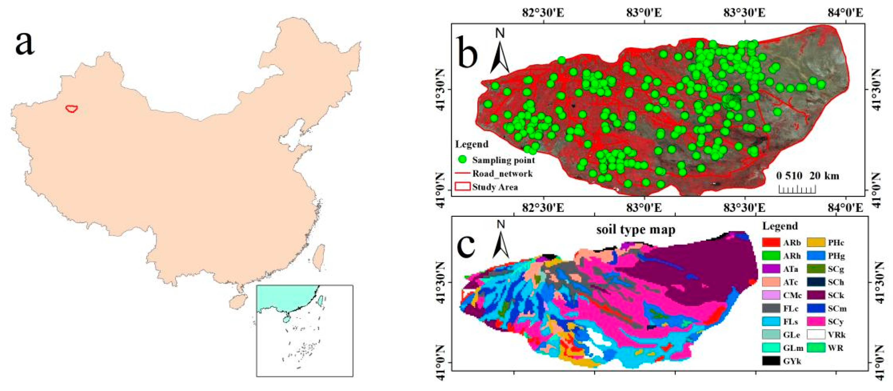
2.1. Study Area

The Werigan–Kuqa River Delta Oasis encompasses the oasis and adjacent areas of Kuqa City, Xinhe County, and Shaya County in the Aksu region, which is located in the southern Tianshan Mountain area in Xinjiang, China (40°57′ N–41°49′ N and 82°9′ E–84°0′ E, Figure 1). The study area belongs to a typical temperate continental climate zone with high evaporation and low rainfall. The primary vegetation types across the study area are halophytic plants, such as Tamarix spp., Halocnemum strobilaceum, and Kalidium foliatum. The dominant soil types are meadow and brown soil, both of which are fine-grained, have low permeability to water, high underground water level, and high mineralization. Due to the drought-prone conditions, irrigation activities, and shallow groundwater depth in the desert oasis transition zone, soil salinization is widespread in the study area [26,27].

2.2. Electrical Conductivity Data Collection

We collected evenly distributed topsoil samples from the research area after fully considering the heterogeneity of the geographical space, soil properties, and vegetation types (Figure 1). Each sample point was divided into a 30 × 30 m rectangular area. Soil samples were then collected at the four corners and center points. Each sample weighed approximately 500 g, and the five samples were evenly mixed to generate the final sampling mixture. The samples were returned to the laboratory, naturally air-dried, ground, and sieved using a 2 mm screen. Next, a 1:5 soil-to-water suspension was prepared at 25 °C, and the electrical conductivity (EC1:5) and SSC were measured using a WTW Multi3420 Set B instrument (WTW, Germany). The sampling campaigns were conducted in August 2005 (6 points), July 2006 (37 points), July 2007 (44 points), September 2008 (73 points), October 2010 (53 points), October 2011 (54 points), August 2013 (37 points), July 2014 (38 points), July 2015 (36 points), April 2016 (39 points), July 2017 (65 points), October 2020 (55 points), and July 2021 (123 points). However, based on the lowest number of sample points collected each year, the arid research area, and low changeability in the climate environment, we combined the data from 2005 to 2021 to obtain adequate data to conduct our salinization research.

2.3. Image Data

The annual Landsat series of remote sensing images (2001–2021) were obtained using the Google Earth Engine (GEE) [28]. Considering the continuous time series, the image for July of each year was obtained to determine the SSC for those months.

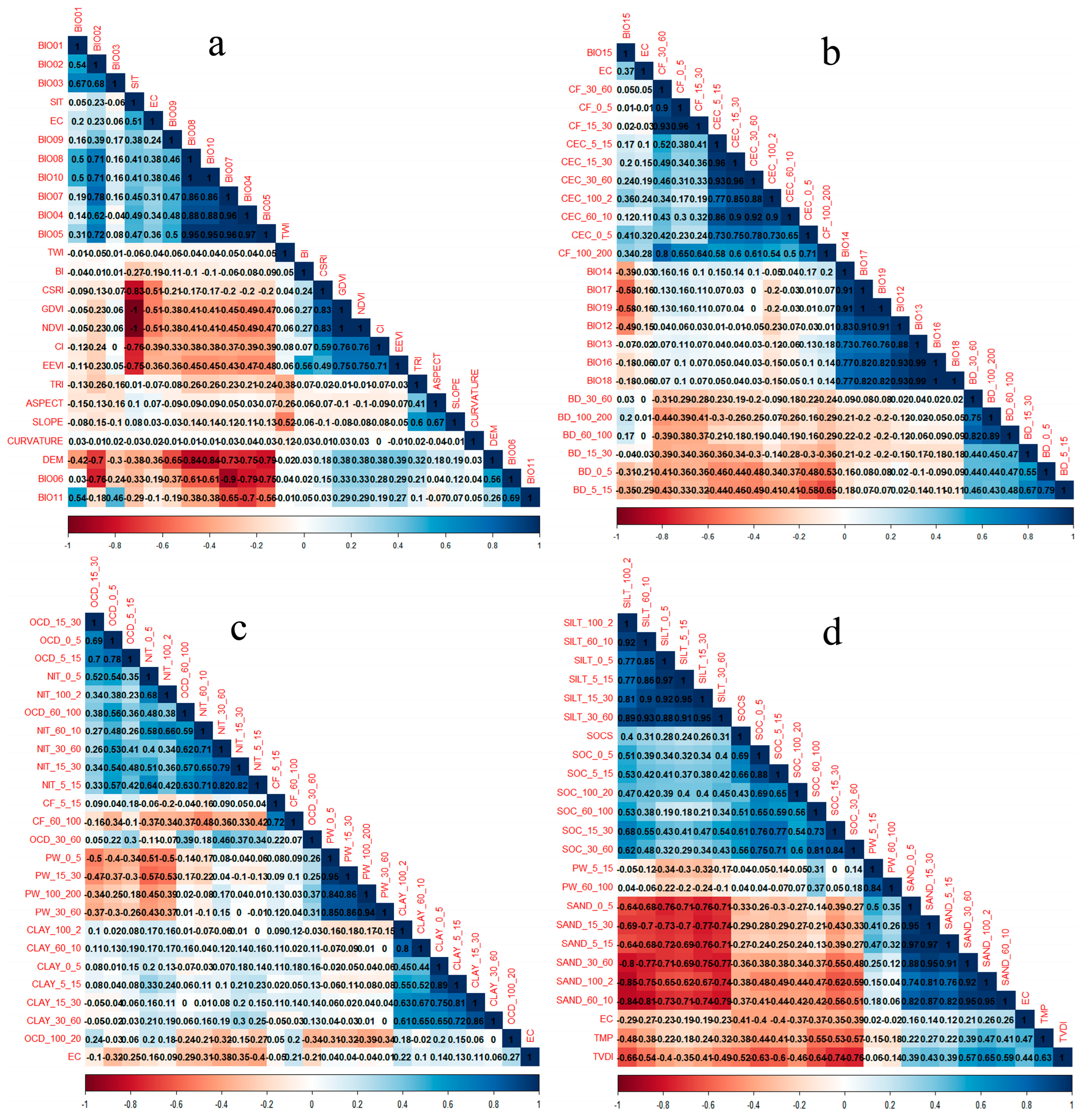
2.4. Environmental Factors

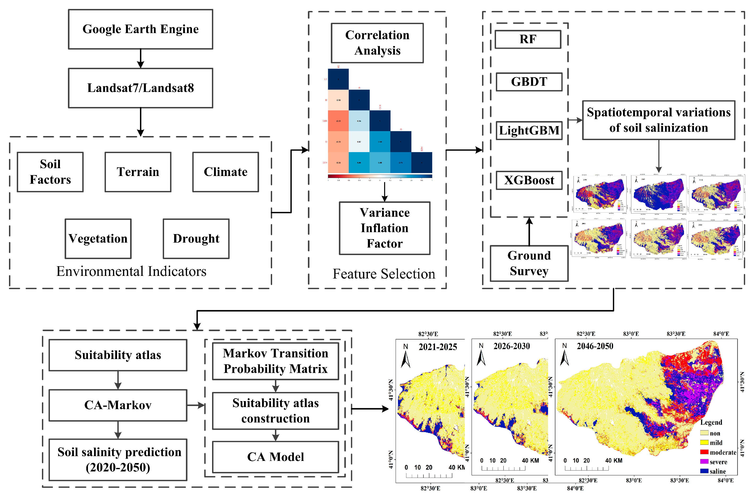
Environmental variables were selected mainly based on Jenny’s soil formation theory, the SCORPAN framework (soil, climate, organic matter, biological factors, terrain, parent material, time, and space), and the corresponding literature [8,23,25,29,30,31,32] (

Table 1. Spatiotemporal predictors of soil salinity.

Auxiliary Data	Environmental Covariates and Abbreviations	Original Resolution and Expression	Source	Reference
Terrain attributes	Digital elevation model (DEM)	30 m	ASTER GDEM NASA	2
	Slope	30 m	SAGA GIS	2
	Aspect	30 m	SAGA GIS	2
	Topographic wetness index (TWI)	30 m 30 m	SAGA GIS	2
	Topographic relief index (TRI)	30 m	SAGA GIS	2
Soil properties	Clay content (Clay)	250 m 1	SAGA GIS	3
	Soil organic carbon (SOC)	250 m	SAGA GIS	3
	Bulk density (BD)	250 m	SAGA GIS	3
	Cation exchange capacity (CEC)	250 m	SAGA GIS	3
	Sand content (Sand)	250 m	SAGA GIS	3
	Silt content (Silt)	250 m	SAGA GIS	3
	Coarse fragments (CFs)	250 m	SAGA GIS	3
	Nitrogen (Nit)	250 m	SAGA GIS	3
	Organic carbon density (OCD)	250 m	SAGA GIS	3
	pH water (PW)	250 m	SAGA GIS	3
	Soil organic carbon stock (SOCS)	250 m	SAGA GIS	3
Climate	Precipitation (PRE)	25 km	TRMM 3B43	3
	Temperature (TMP)	1 km	MOD11A2 NASA	3
	Bioclimatic variables (Bio 1, Bio 2, Bio 3, … Bio 19)	1 km	www.worldclim.org accessed on 19 September 2023	4
Salinity index	SI-T (Salinity index)	30 m $\left(\mathrm{R}-\mathrm{N}\mathrm{I}\mathrm{R}\right)$ × 100	Landsat5/7/8	4
	BI (Brightness index)	ditto $\sqrt{{\mathrm{R}}^2+{\mathrm{N}\mathrm{I}\mathrm{R}}^2}$	Landsat5/7/8	4
Vegetation index	NDVI (Normalized differential vegetation index)	ditto $\frac{\mathrm{N}\mathrm{I}\mathrm{R}-\mathrm{R}}{\mathrm{N}\mathrm{I}\mathrm{R}+\mathrm{R}}$	Landsat5/7/8	4
	EVI (Enhanced vegetation index)	ditto $2.5\times \frac{\left(\mathrm{N}\mathrm{I}\mathrm{R}+{\mathrm{S}\mathrm{W}\mathrm{I}\mathrm{R}}_1-\mathrm{R}\mathrm{E}\mathrm{D}\right)}{\left(\mathrm{N}\mathrm{I}\mathrm{R}+{\mathrm{S}\mathrm{W}\mathrm{I}\mathrm{R}}_1+6\times \mathrm{R}\mathrm{E}\mathrm{D}-7.5\times \mathrm{B}+1\right)}$	Landsat5/7/8	4
	GDVI (Generalized difference vegetation index)	ditto $\frac{{\mathrm{N}\mathrm{I}\mathrm{R}}^{\mathrm{n}}-{\mathrm{R}}^{\mathrm{n}}}{{\mathrm{N}\mathrm{I}\mathrm{R}}^{\mathrm{n}}+{\mathrm{R}}^{\mathrm{n}}}$	Landsat5/7/8	4
	CRSI (Canopy response salinity index)	ditto $\sqrt{\frac{\left(\mathrm{N}\mathrm{I}\mathrm{R}\times \mathrm{R}\right)-\left(\mathrm{G}\times \mathrm{B}\right)}{\left(\mathrm{N}\mathrm{I}\mathrm{R}\times \mathrm{R}\right)+\left(\mathrm{G}\times \mathrm{B}\right)}}$	Landsat5/7/8	4
Drought Index	TVDI (Temperature vegetation drought index)	ditto $\frac{{\mathrm{T}}_{\mathrm{s}}-{\mathrm{T}}_{\mathrm{m}\mathrm{i}\mathrm{n}}}{{\mathrm{T}}_{\mathrm{m}\mathrm{a}\mathrm{x}}-{\mathrm{T}}_{\mathrm{m}\mathrm{i}\mathrm{n}}}$ Tmax = a + b × NDVI Tmin = c + d × NDVI a, b, c, and d are the fitting coefficients of the dry and wet line	Landsat5/7/8	5

¹ Six different depths: 0–5 cm, 5–15 cm, 15–30 cm, 30–60 cm, 60–100 cm, and 100–200 cm. ² Taghizadeh-Mehrjardi et al., 2021; Taghizadeh-Mehrjardi et al., 2014 [10,30]. ³ Hassani et al., 2021 [23]. ⁴ Wang et al., 2021; Wang et al., 2017 [29,32]. ⁵ Sandholt et al., 2002 [31].

). The variables used to predict soil salinity included the vegetation, soil, climate, and terrain data. The vegetation- and salinity-related indicators (NDVI, enhanced vegetation index (EVI), generalized difference vegetation index (GDVI), canopy response salinity index (CRSI), salinity index (SI-T), and brightness index (BI)) were calculated from Landsat 5/7/8 image data, which were captured using GEE. Precipitation, temperature, and 19 types of bioclimatic variables were used as climate-related parameters. These biological variables represent the annual change or restrictive environmental indicators, such as the average annual temperature and precipitation and are important influencing factors for predicting soil salinization [29]. The soil-related information included the multi-depth (0–200 cm) clay content, bulk density, and soil organic carbon (data obtained from SoilGrids) [33]. The ASTER GDEM from NASA was used to derive terrain-related covariates that were calculated using SAGA-GIS [10] (Table 1), including the slope, aspect, and topographic wetness index (TWI). The temperature vegetation drought index (TVDI) can effectively monitor drought conditions and reflects the spatial distribution characteristics of soil moisture [34]. It has been widely used for drought monitoring and for predicting soil salinization [35,36]. Then, we calculated the correlation between these environmental variables and SSC and generated a correlation coefficient matrix (Figure 2). As the initial number of environmental variables reached 95, displaying the correlation between variables on one graph produces results with an extremely crowded appearance not conducive to analysis. Therefore, we divided every 24 variables into a group to analyze the correlation between variables, as shown in Figure 2. The correlation coefficient matrix shows a significant correlation problem between different types of environmental variables (Figure 2), with a strong correlation (>0.5) observed between variables of the same type, such as bioclimatic variables, vegetation indices, and soil properties. Therefore, we calculated the variance inflation factor (VIF) between different indicators to analyze the multicollinearity [37]. All environmental predictors in Table 1 were considered for screening the variables according to a criterion of VIF < 10. These screened variables were used as input factors for the four ML methods (RF, LightGBM, GBDT, and XGBoost).

2.5. Methods

First, the environmental variables were screened using the VIF. Second, the soil salinity content was predicted with the aid of several ML methods (RF, GBDT, LightGBM, XGBoost) using the screened variables as input indicators. The spatiotemporal variations in soil salinization were analyzed. These methods all belong to ensemble learning, which is a technique that can improve the generalization ability and robustness of a single learner by combining the prediction results of multiple base learners [38]. These methods have been used by numerous studies to estimate soil salinization, whose results indicate that these methods have high accuracy and strong robustness [39,40,41,42]. However, few studies compare the accuracy of these methods at the same time. Therefore, we used these methods to conduct research on soil salinization to find the optimal modeling method. In addition, we detail the advantages and characteristics of each method in Section 2.5.1, Section 2.5.2, Section 2.5.3, Section 2.5.4 and Section 2.5.5. Third, future soil salinity was simulated using the CA–Markov model. We chose the CA–Markov model because it combines the advantages of simulating spatial changes and performing long-term predictions of complex systems; it possesses outstanding advantages in spatiotemporal forecasting [24,25]. Furthermore, recent research has shown that the CA–Markov Model paired with RS and GIS is a valuable and robust modeling tool for the transition and future projections of LULC, which can provide comprehensive information on a large-scale synoptic level [43]. Figure 3 shows the research concepts presented in this study.

2.5.1. Random Forest

The RF algorithm is an outstanding ML technology for DSM that has a powerful modeling ability, recommended for simulating soil salinization in arid regions [41,44]. The RF model has been successfully applied to predict soil organic carbon, soil parent material, groundwater depth, and soil moisture [29]. The advantage of the RF algorithm is the ease of application, and the default method was used to avoid over-fitting. Furthermore, it can be used to process high–dimensional data [45]. The RF algorithm was built based on the RF software (v0.0) package in Python (v3.6.13). Additionally, the Boruta algorithm, which is a wrapper built around the RF, was used to estimate the covariate’s importance [46,47].

2.5.2. Gradient Boosting Decision Tree

The Gradient Boosting Decision Tree (GBDT) is a boosting ensemble algorithm obtained by integrating multiple classification and regression trees (CARTs), which are included as decision trees [48]. GBDT uses the gradient descent method for optimization that has gradient boosting (GB) and decision tree (DT) functional characteristics, and it has a good training effect and prevents overfitting [49]. The main computational cost of the GBDT method is learning the decision tree, and the most time-consuming part is discovering the optimal segmentation point [48]. Assuming that the training set has n independent identically distributed samples and each x_i is a vector in the feature space, the negative gradient of the output of the loss function of the model is expressed as $\left\{g_1,..g_n\right\}$:

$$-{\mathrm{g}}_{\mathrm{m}}\left({\mathrm{x}}_{\mathrm{i}}\right)=-\left[\frac{\partial \mathrm{L}\left({\mathrm{y}}_{\mathrm{i}},\mathrm{F}\left({\mathrm{x}}_{\mathrm{i}}\right)\right)}{\partial \mathrm{F}\left({\mathrm{x}}_{\mathrm{i}}\right)}\right]\mathrm{F}(\mathrm{x})={\mathrm{F}}_{\mathrm{m}-1}(\mathrm{x})$$

(1)

where $\mathrm{L}\left({\mathrm{y}}_{\mathrm{I}},\mathrm{F}\left({\mathrm{x}}_{\mathrm{i}}\right)\right)$ is the loss function and $\mathrm{F}\left({\mathrm{x}}_{\mathrm{i}}\right)$ is the regression tree.

The decision tree model uses the most informative features to segment each node. In this study, the GBDT model was implemented based on the sklearn.ensemble.GradientBoostingRegressor class of scikit-learn in Python.

2.5.3. Light Gradient Boosting Machine

The Light Gradient Boosting Machine (LightGBM) is an improved algorithm in the gradient enhancement framework and GBDT model proposed by the Microsoft DMTK team. This algorithm has a high training speed and low memory requirements, thereby greatly accelerating training and significantly improving simulation accuracy [50]. LightGBM solves the problems of low training efficiency and poor scalability for high latitudes and big data by introducing two technologies, Gradient-based One Side Sampling (GOSS) and Exclusive Feature Bundling (EFB) [51]. Through GOSS, a large portion of data samples with smaller gradients can be excluded, and only the remaining samples can be used to predict information gain. By bundling mutually exclusive features together through EFB, the number of features can be reduced. This study implemented the GBDT model based on the LightGBM framework within Python.

2.5.4. EXtreme Gradient Boosting

The EXtreme Gradient Boosting (XGBoost) algorithm based on the gradient lifting method introduces a regularization term based on the traditional boosting algorithm to better control model complexity [52]. It is also based on the gradient-boosting algorithm, which has the following advantages: fast operation speed, good effect, easy parameter adjustment, and massive data processing [53]. Compared to other machine learning algorithms, it has stronger interpretability. The core algorithm concept of XGBoost is to improve the overall prediction performance of the model by gradually adding trees to the model. The objective function of XGBoost is divided into loss function and regularization terms [54]. The loss function term reveals the training error, while the regularization term defines the complexity, avoids overfitting, and minimizes the calculation cost; further, it will automatically perform parallel computing during the training process. In the XGBoost algorithm, the square loss is constructed as the objective function for the regression problem, the binomial expansion of the objective function is performed with a Taylor series to solve the problem of optimization difficulty in the objective function, and the gradient descent algorithm is used to optimize the solution [55]. In this study, the XGBoost model was implemented based on the XGBoost library for Python.

2.5.5. CA–Markov Model for Predicting Future Soil Salinization

The CA–Markov model integrates the advantages of both the Markov and CA models, with outstanding effects in the spatiotemporal prediction of scene changes [56]. We used the CA–Markov model in the IDRISI software (vIDRISI 17.0) to predict future soil salinity change patterns.

The CA is defined as a discrete dynamic model, which has evolved into a global change model in time and space based on the local behavior between individuals [57]. It can simulate complex natural phenomena and is widely used to investigate land use, urban growth patterns, fire simulations, and other fields [25]. The conceptual model of CA can be expressed as follows [58]:

$$S_{i,t+1}=f\left(S_{i,t},P_0,{\Omega }_{i,m},CONS,RND\right)$$

(2)

where S_i,t and S_i,t+1 represent the state of the cell at time t and t + 1 at spatial position i, respectively; f is the conversion function; P₀ represents the overall conversion probability; and ${\Omega }_{i,m}$ represents the m × m window size of the neighborhood effect. Moreover, CONS defines the constrained region. If a cell can be converted, then it is assigned a value of 1; otherwise, it is assigned a value of 0. Finally, RND represents the unknown random disturbance.

The Markov chain is a random process without an after effect [56], and it can predict future trends through the initial probability of different categories and the transition probability between categories. The change process of salinized land can be regarded as a Markov process (in this study, we refer to various salinized soil types). Therefore, the following conceptualized formula can simulate the state of the soil salinity type:

S_(t+1) = p_i,j × S_(t)

(3)

$${\mathrm{P}}_{\mathrm{i},\mathrm{j}}=\left\{\begin{array}{l}{\mathrm{P}}_{11}{\mathrm{P}}_{12}\cdot \cdot \cdot {\mathrm{P}}_{1\mathrm{n}}\\ {\mathrm{P}}_{21}{\mathrm{P}}_{22}\cdot \cdot \cdot {\mathrm{P}}_{2\mathrm{n}}\\ \cdot \cdot \cdot \cdot \cdot \cdot \cdot \cdot \cdot \cdot \cdot \cdot \\ {\mathrm{P}}_{\mathrm{n}1}{\mathrm{P}}_{\mathrm{n}2}\cdot \cdot \cdot {\mathrm{P}}_{\mathrm{nn}}\end{array}\right\}$$

(4)

where S_(t) and S_(t+1) represent the state of the soil salinized type at t and t + 1, respectively, P_i,j is the state transition matrix; and S_(t+1) is the predicted result of salinization.

2.5.6. Suitability Atlas Construction and Prediction Process

The number of and spatial changes in the soil salinity type were predicted using the IDRISI software. The main process was as follows [59]. (1) The Markov transfer probability matrix and transfer area were obtained based on salinized land types in two historical periods (such as 2005–2010). The period was set to 5 years, and a suitability atlas was generated. (2) The “Decision Wizard” module was used to prepare the suitability dataset. Soil-, climate-, and vegetation-related variables were included in the suitability atlas. (3) The soil-salinity-type image of the study area in the target year (such as 2015) was simulated. For example, using 2010 as the base year, the land use transfer area matrix from 2005 to 2010 was established in the first step, the suitability dataset used was obtained in the second step, and the iteration number was 5. Then, the predicted classification map of soil salinization in 2015 was simulated. (4) The “Crosstab” module in IDRISI was used for accuracy verification, the predicted map was compared with the actual salinized type (such as 2010), and the Kappa coefficient was calculated. According to the unique geographical features of the research area and the characteristics of the soil salinity spatial pattern, the soil-, climate-, and vegetation-related variables were all key factors applied in the CA–Markov model (Table 1).

2.5.7. Trend Analysis Method

We used a linear equation to quantify the salt content trends [60], with the years (t) set as a factor of time and the SSC (y) set as the predicted value to establish the linear regression equation for t and y:

y = b + at

(5)

$$\mathrm{a}=\frac{\mathrm{n}\times {\displaystyle \sum _{\mathrm{i}=1}^{\mathrm{n}}(\mathrm{i}\times {\mathrm{P}}_{\mathrm{i}})}-{\displaystyle \sum _{\mathrm{i}=1}^{\mathrm{n}}\mathrm{i}}{\displaystyle \sum _{\mathrm{i}=1}^{\mathrm{n}}{\mathrm{P}}_{\mathrm{i}}}}{\mathrm{n}\times {\displaystyle \sum _{\mathrm{i}=1}^{\mathrm{n}}{\mathrm{i}}^2-{({\displaystyle \sum _{\mathrm{i}=1}^{\mathrm{n}}\mathrm{i}})}^2}}$$

(6)

where a is the slope of the interannual change in the SSC, n represents the number of years, and P_i is the SSC value in the ith year. Additionally, a indicates the trend in the SSC, where a value greater than zero indicates an increasing trend in soil salt content, and a × 10 indicates the tendency rate, where the unit is (g/kg)/10 years.

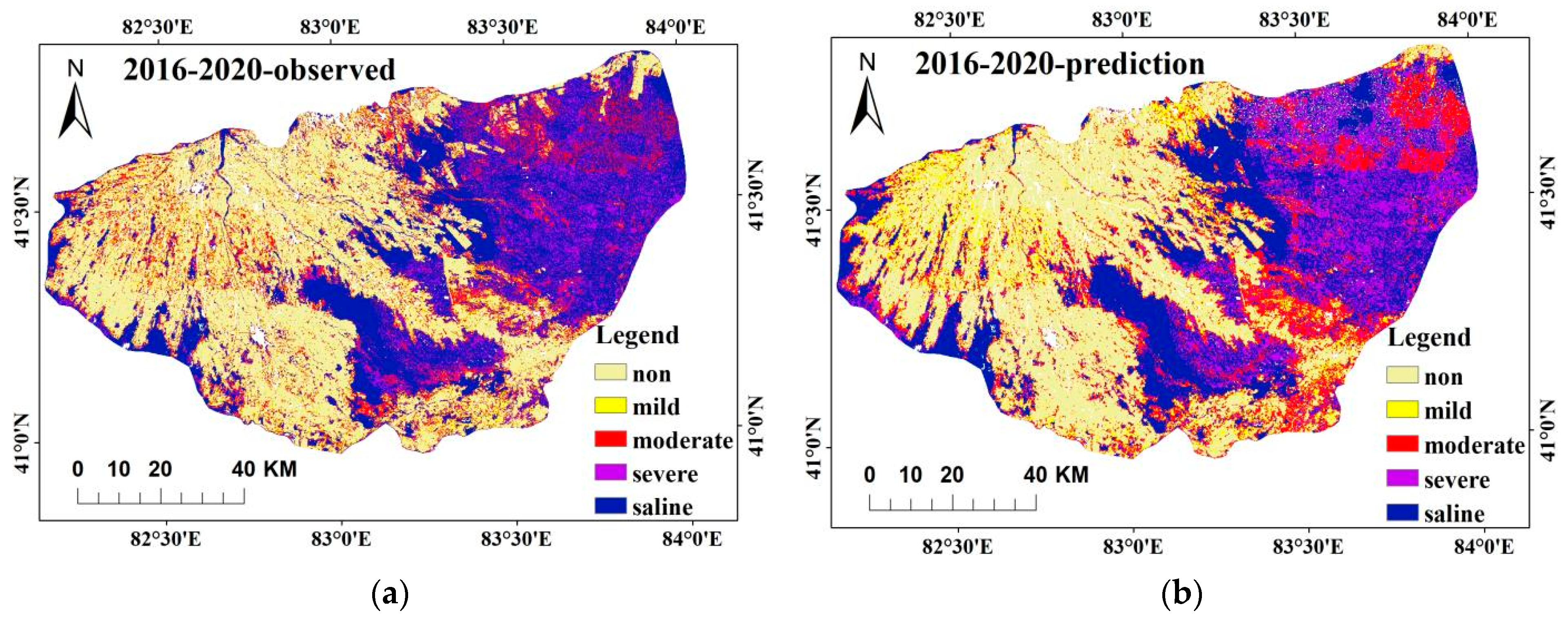
2.5.8. Model Validation

The root mean square error (RMSE), coefficient of determination (R²), ratio of performance to interquartile distance (RPIQ), and mean absolute error (MAE) were used to evaluate the prediction accuracy of the SSC [45,52]:

$$\mathrm{RMSE}=\sqrt{\frac{1}{\mathrm{n}}{\displaystyle \sum _{\mathrm{i}=1}^{\mathrm{n}}{{(\mathrm{O}}_{\mathrm{i}}-{\mathrm{P}}_{\mathrm{i}})}^2}}$$

(7)

$${\mathrm{R}}^2={\left[\frac{{\displaystyle \sum _{\mathrm{i}=1}^{\mathrm{n}}({\mathrm{O}}_{\mathrm{i}}-{\mathrm{O}}_{\mathrm{ave}})({\mathrm{P}}_{\mathrm{i}}-{\mathrm{P}}_{\mathrm{ave}})}}{{\sqrt{{\displaystyle \sum _{\mathrm{i}=1}^{\mathrm{n}}{({\mathrm{O}}_{\mathrm{i}}-{\mathrm{O}}_{\mathrm{ave}})}^2{({\mathrm{P}}_{\mathrm{i}}-{\mathrm{P}}_{\mathrm{ave}})}^2}}}_{}}\right]}^2$$

(8)

$$\mathrm{R}\mathrm{P}\mathrm{I}\mathrm{Q}=\frac{∆\mathrm{Q}}{\mathrm{R}\mathrm{M}\mathrm{S}\mathrm{E}}$$

(9)

$$\mathrm{MAE}=\frac{1}{\mathrm{n}}{\displaystyle {\sum }_{\mathrm{i}=1}^{\mathrm{n}}{|\mathrm{O}}_{\mathrm{i}}-{\mathrm{P}}_{\mathrm{i}}|}$$

(10)

where P_i represents the predicted values; O_i indicates the observation results; O_ave and P_ave are the average observed and predicted values, respectively; $∆\mathrm{Q}$ is the interquartile range (IQR), which is the difference between the upper quartile (Q₃) and the lower quartile (Q₁); and n is the number of data.

2.6. Soil Salinization Classification

Based on the linear relationship between our statistical electrical conductivity (EC, dS m⁻¹) and SSC (g/kg) where SSC = EC × 0.6763 − 0.4988, the predicted EC was converted to SSC. The Werigan–Kuqa River Delta Oasis is located at the southern foot of the Middle Tianshan Mountains and is an alluvial fan formed by the accumulation of flowing water. Under this terrain condition, chloride-sulfate and sulfuric acid saline soils easily form; the salinization type in the research area belongs to this type [61]. Therefore, this study classified soil salinization in Xinjiang into five levels based on the chloride-sulfate grading standard in the second soil census of Xinjiang: non saline < 8 g/kg; 8 g/kg < mildly saline < 10 g/kg; 10 g/kg < moderately saline < 15 g/kg; 15 g/kg < severely saline < 20 g/kg; and saline oil > 20 g/kg [16,62,63,64].

3. Results and Discussion

3.1. Accuracy Evaluation

The prediction results show that LightGBM had the highest RPIQ and lowest MAE and RMSE (MAE = 9.20, RMSE = 11.88, R² = 0.73, and RPIQ = 3.08), followed by GBDT (MAE = 8.43, RMSE = 12.84, R² = 0.72, and RPIQ = 3.02). Meanwhile, XGBoost had stronger predictive power than RF (lower RMSE, MAE, higher R², and RPIQ). Therefore, the above analysis indicates that the overall model prediction accuracy can be ranked as LightGBM > GBDT > XGBoost > RF (

Table 2. Accuracy comparison results of the different models based on the validation set.

Algorithm	MAE (dS m−1)	RMSE (dS m−1)	R2	RPIQ
RF	9.23	12.84	0.68	2.86
XGBoost	8.77	12.30	0.71	2.98
GBDT	8.43	12.15	0.72	3.02
LightGBM	9.20	11.88	0.73	3.08

). Accordingly, soil salinization predictions using the LightGBM model are presented in the subsequent sections.

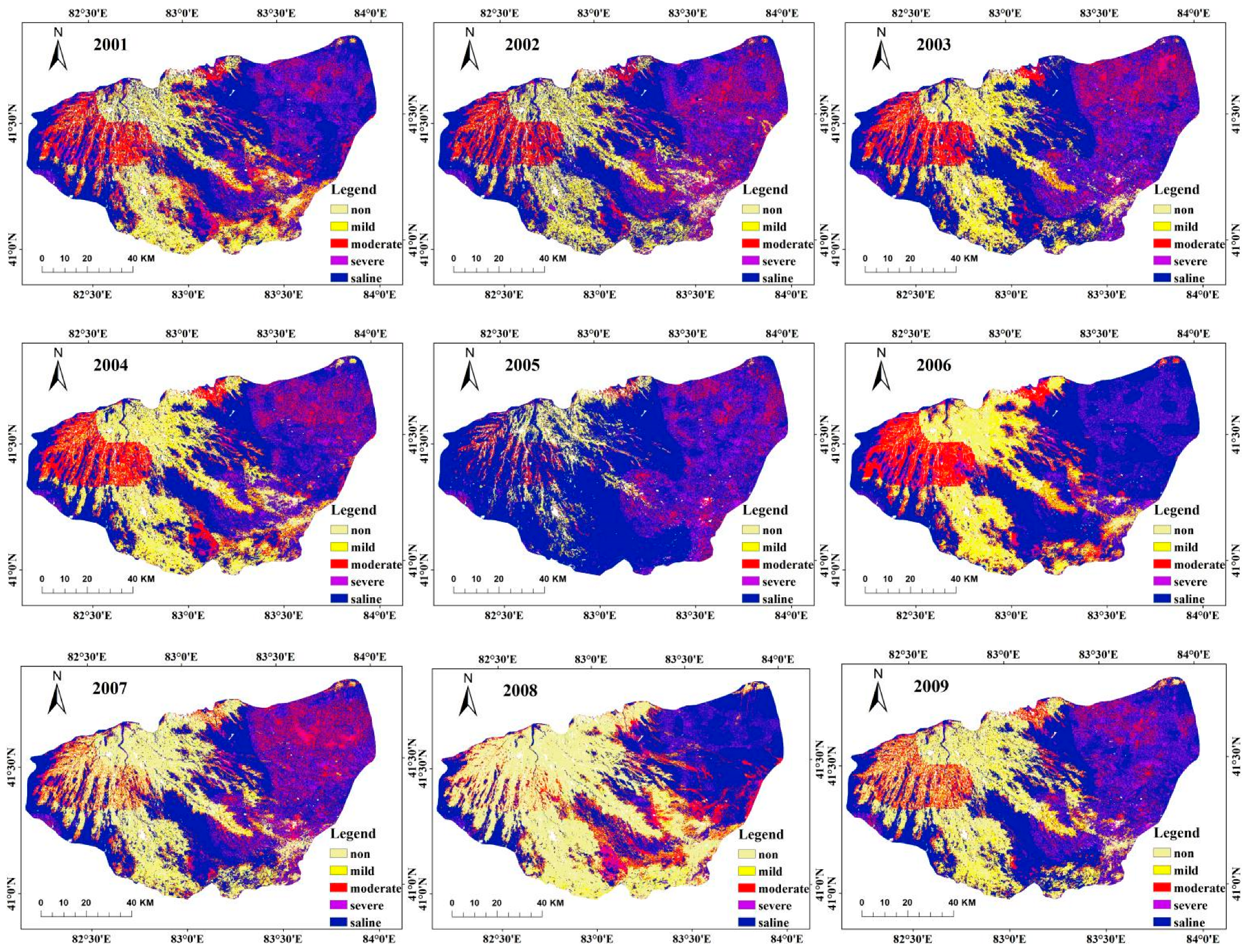
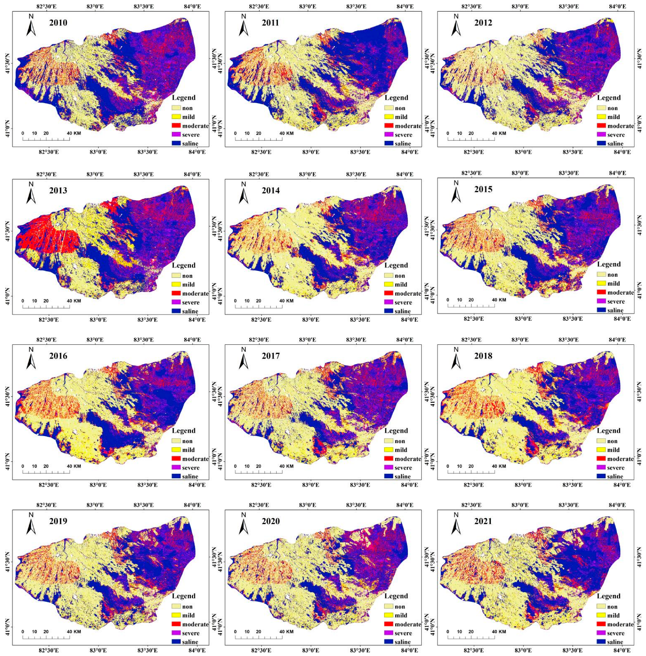
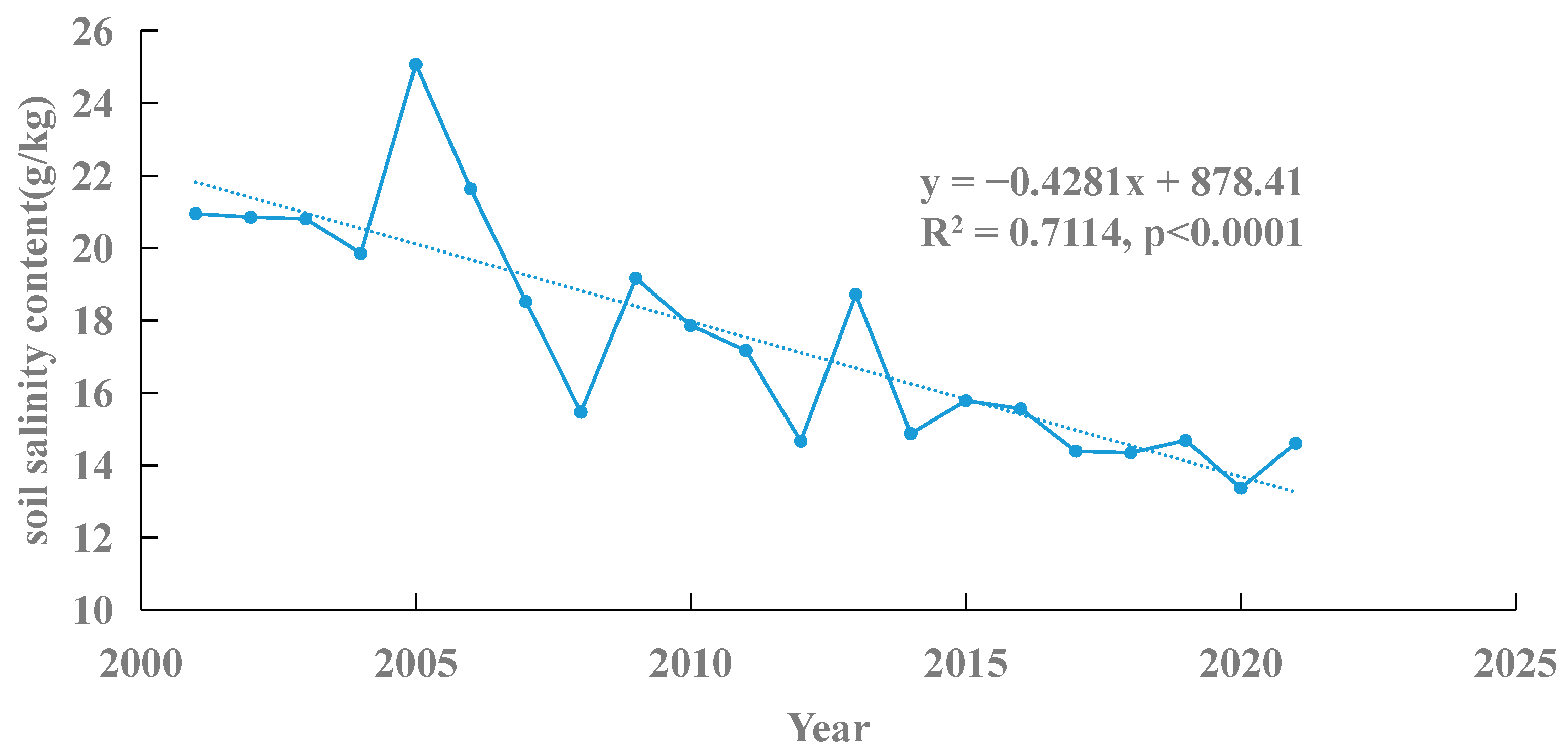
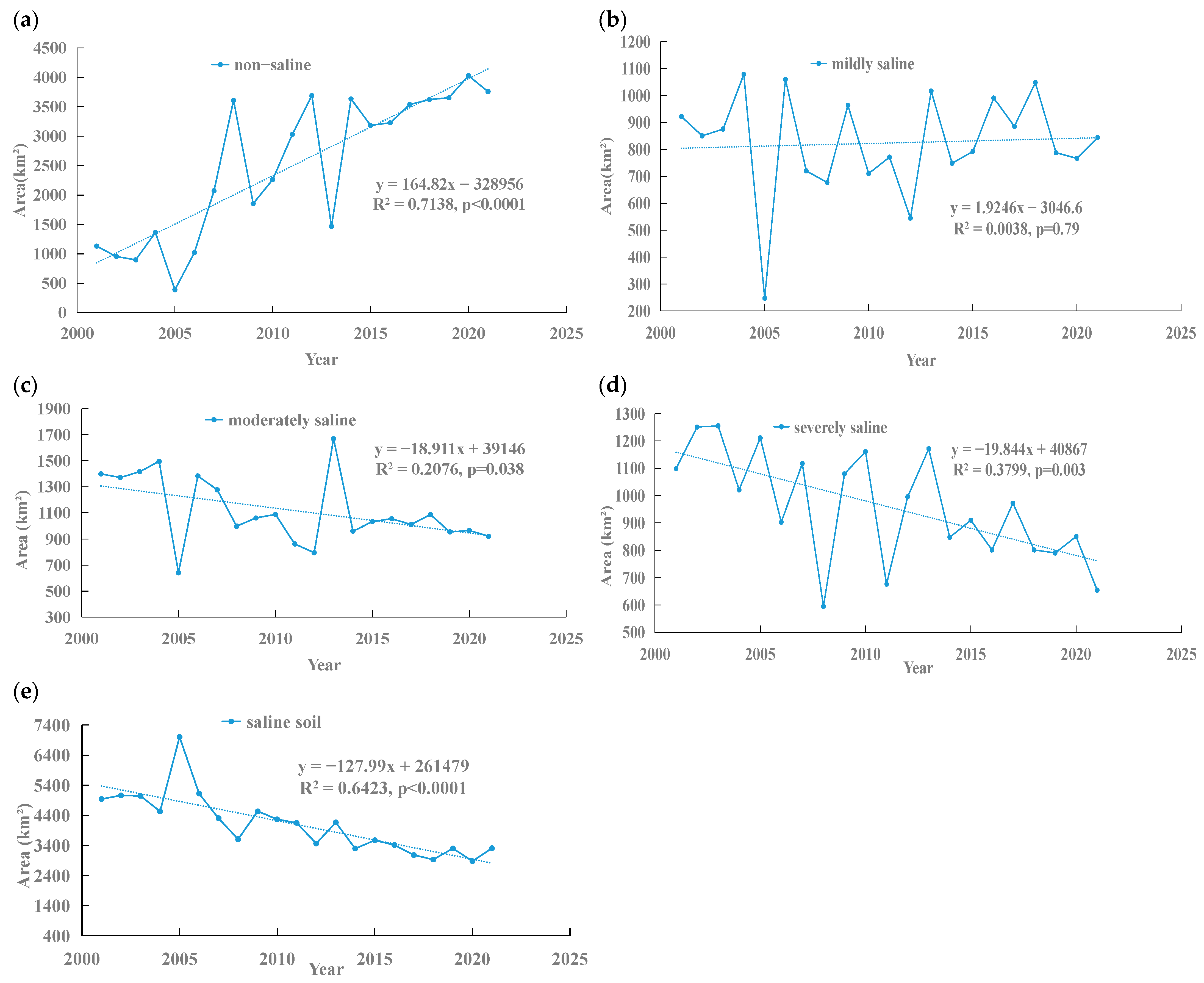
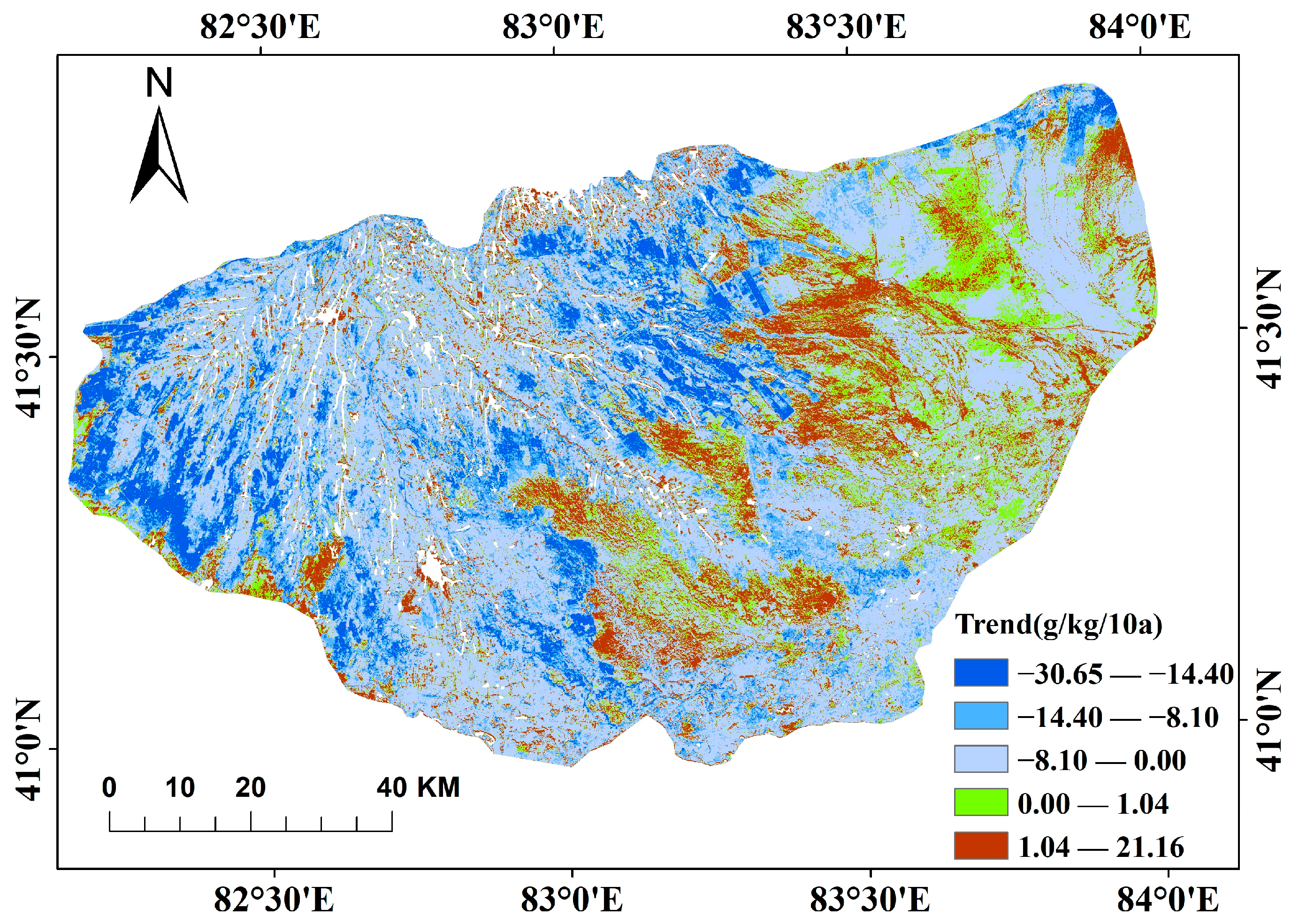
3.2. Spatiotemporal Variation in Soil Salinity

The average SSC from 2001 to 2021 was 1.19–46.82 g/kg, and the inter-annual average was 17.54 g/kg (Figure 4). Significant differences were observed in the area and were proportional to soil salinization at different levels in different years, such as moderate salinization ranging from 641.36 km² (2005) to 1669.36 km² (2013), which accounted for a range of 6.76–17.59% (Figure 4,

Table 3. Area and proportion of soil salinization from 2001 to 2021 (unit: km²).

Year	Non	Proportion (%)	Mild	Proportion (%)	Moderate	Proportion (%)	Severe	Proportion (%)	Saline Soil	Proportion (%)
2001	1131.08	11.92	921.69	9.71	1399.18	14.74	1098.56	11.58	4939.35	52.05
2002	954.83	10.06	850.29	8.96	1371.61	14.45	1250.80	13.18	5062.32	53.34
2003	897.37	9.46	874.99	9.22	1416.00	14.92	1255.27	13.23	5046.22	53.17
2004	1363.80	14.37	1078.87	11.37	1496.00	15.76	1020.53	10.75	4530.65	47.74
2005	388.09	4.09	247.31	2.61	641.36	6.76	1211.02	12.76	7002.08	73.78
2006	1020.62	10.75	1059.37	11.16	1383.15	14.58	902.30	9.51	5124.41	54.00
2007	2074.65	21.86	720.06	7.59	1277.27	13.46	1117.33	11.77	4300.54	45.32
2008	3611.34	38.05	677.09	7.13	998.06	10.52	595.75	6.28	3607.62	38.02
2009	1854.19	19.54	963.20	10.15	1060.48	11.17	1079.45	11.37	4532.53	47.76
2010	2264.21	23.86	710.27	7.48	1087.28	11.46	1160.39	12.23	4267.71	44.97
2011	3032.65	31.96	771.00	8.12	862.35	9.09	676.52	7.13	4147.33	43.70
2012	3690.54	38.89	544.62	5.74	795.26	8.38	995.56	10.49	3463.88	36.50
2013	1467.16	15.46	1016.68	10.71	1669.36	17.59	1171.24	12.34	4165.42	43.89
2014	3633.70	38.29	748.35	7.89	961.02	10.13	848.17	8.94	3298.62	34.76
2015	3183.97	33.55	792.19	8.35	1032.56	10.88	909.60	9.59	3571.54	37.64
2016	3228.45	34.02	990.53	10.44	1054.50	11.11	801.97	8.45	3414.40	35.98
2017	3538.40	37.29	886.08	9.34	1010.28	10.65	971.84	10.24	3083.26	32.49
2018	3622.58	38.17	1047.77	11.04	1086.43	11.45	801.80	8.45	2931.28	30.89
2019	3652.81	38.49	787.52	8.30	955.54	10.07	790.66	8.33	3303.33	34.81
2020	4029.61	42.46	766.48	8.08	966.27	10.18	850.80	8.97	2876.69	30.31
2021	3759.59	39.62	843.86	8.89	922.32	9.72	654.52	6.90	3309.56	34.87
mean	2495.22	26.29	823.72	8.68	1116.49	11.77	960.19	10.12	4094.23	43.14

). Severely saline and saline soil were dominant east and south of the Werigan–Kuqa River Delta Oasis, with an average area of 1833.55 km² (occupying 19.32%) and 3631.30 km² (occupying 38.27%), respectively (Figure 4). The southern part of the research area is adjacent to the Tarim River, which largely accounts for the higher groundwater level in the area. Furthermore, the strong evaporation effect led to the accumulated salinity content through the movement of the soil salinity along with the water. The moderately saline conditions were mainly distributed in the northern and western regions over an area of 1116.49 km² (occupying 16.30%). The inner oasis had the lowest soil salinity, which was dominated by non-saline and mildly saline, with areas of 2495.22 km² (occupying 16.88%) and 823.72 km² (occupying 9.23%), respectively. These observations are consistent with those of previous studies [16,29].

In terms of the temporal distribution, Figure 5 shows that the SSC had a general markedly decreasing trend (p < 0.001), with a decreasing rate of 4.28 g/kg 10 a⁻¹. The wasteland reclamation process was one of the main reasons for the declining trend in salinization. As shown in Figure 4, many wastelands on the outskirts of the oases have been converted into arable land over the past 20 years. The most severe salinization occurred in 2005, with an average SSC of 25.07 g/kg, while the mildest salinization occurred in 2020, with an average value of 13.37 g/kg. The non-saline and mildly saline areas were increasing at a rate of 164.82 and 1.92 km²/a, respectively, and the other salinized soil levels showed a downward trend (Figure 5 and Figure 6). Furthermore, the moderately saline area showed a significantly decreasing trend (18.91 km²/a), and the smallest area was observed in 2005 (641.36 km²). The severely saline area showed a decreasing rate of 19.84 km²/a, which changed sharply before 2014 and then became relatively stable. In 2008, the severely saline area was the smallest, at 595.75 km². Additionally, the saline soil area showed a significant downward trend at a rate of 127.99 km²/a.

Figure 7 indicates that areas with decreasing and increasing trends accounted for 75.04 and 24.96% of the study area, respectively, which implies that the SSC mainly decreased in the research area. Thus, the entire oasis region was mainly associated with a decreasing amplitude of 0.00−14.40 g/kg·10 a⁻¹. Furthermore, soil salinization in the desert region revealed an increasing amplitude of 0.00−21.16 g/kg·10 a⁻¹, while soil salinization in the oasis areas revealed a decreasing amplitude of 0.00−30.65 g/kg·10 a⁻¹. In the oasis area, the farther from built-up areas, the higher the reduction range of the SSC, which exhibited significant hierarchical characteristics in the inner oasis and outer oasis regions, with a range of amplitudes of 0.00−8.10 and 8.1−14.40 g/kg·10 a⁻¹, respectively.

Several studies have analyzed changes in the soil salinization of the study area [16,35]. In summary, soil salinization showed a decreasing trend; non−saline and mild−saline areas increased while saline soil areas decreased; mild−saline areas transformed into non-saline areas; moderately−saline areas mainly transformed into mild−saline areas; and soil salinization decreased in the inner oasis region but increased in the outer oasis region. Therefore, at the macro level, the results are consistent with previous findings (Figure 6 and Figure 7).

Our results showed that soil salinization decreased during the analysis period, which was largely due to the significant developments in water resource management in recent decades, especially those that began in 1992. Due to the implementation of China’s Xinjiang Tarim Agricultural Irrigation and Drainage and Environmental Protection project, the soil salinization of irrigation canals has been effectively controlled, and water and salt have gradually attained a balance [65]. The results further revealed severe soil salinization in some local regions, possibly due to unreasonable water resource utilization, unconscious irrigation, irrigation of agricultural land with saline water, leaking channels, and flood irrigation if the underground water level was too high. These factors can cause soil salinization and swamping, leading to soil salt gathering in the irrigation area [66]. Additionally, the low utilization rate of the plain reservoir and groundwater level around the basin introduces salt from upstream- to downstream-irrigated regions of the research area, which may have led to severe salinization. Furthermore, climate factors may have been involved, such as the dry climate of the research area, the domination of water entering the oasis through evaporation, and limitations of the drainage system in the drainage basin. These reasons could lead to water loss and increase soil salt and the degree of soil salinization [16,67].

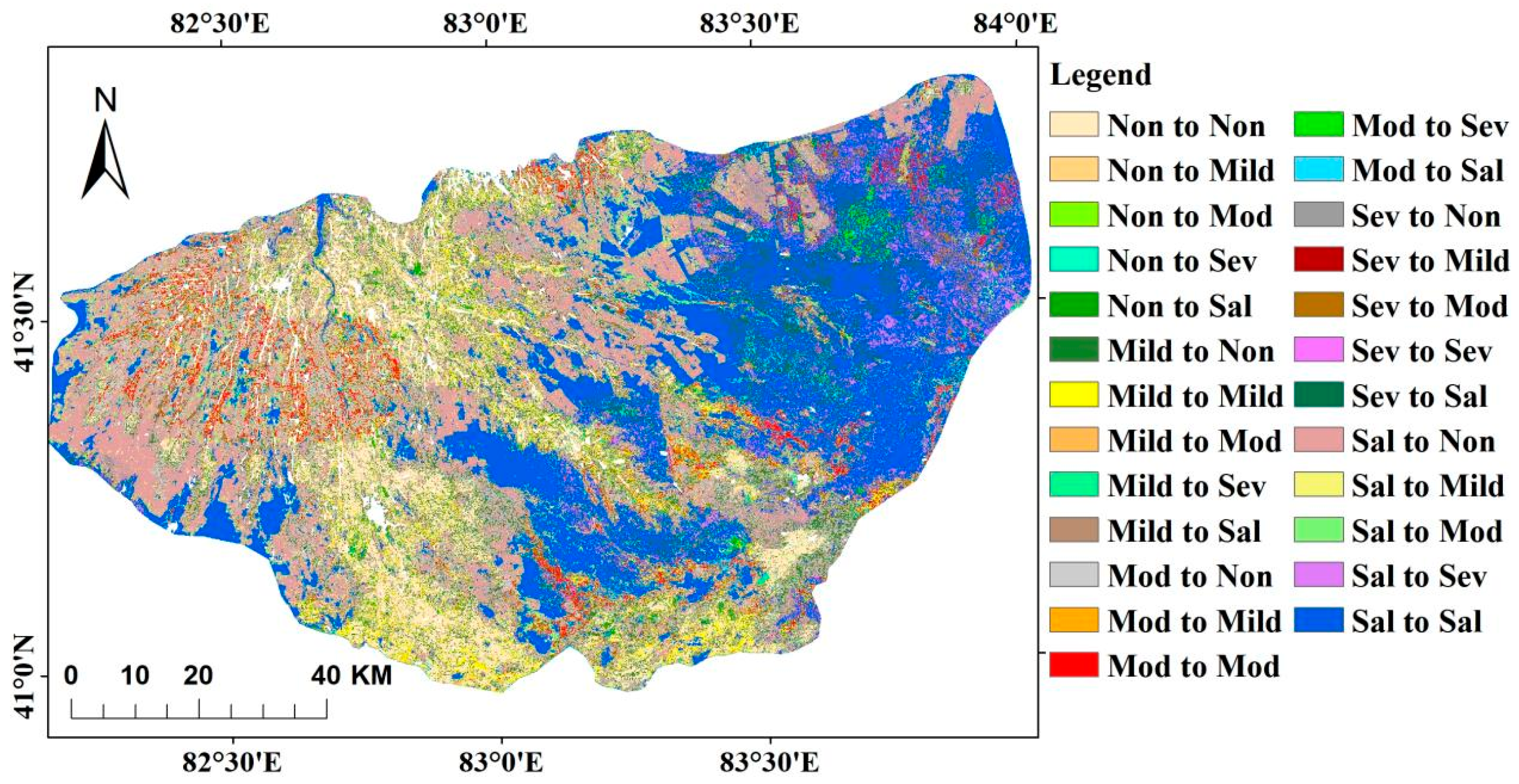
3.3. Transfer Matrix of Soil Salinization

Table 4. Soil salinity type transfer matrix (unit: km²).

	2021	Non	Mild	Moderate	Severe	Saline	Total Area
2001
Non		886.95	87.85	35.31	13.42	107.54	1131.08
Mild		521.88	241.52	46.53	15.70	96.05	921.69
Moderate		665.74	153.34	293.97	91.18	194.95	1399.18
Severe		258.66	68.76	155.07	292.09	323.97	1098.56
Saline		1426.37	292.38	391.43	242.13	2587.05	4939.35
Total Area		3759.59	843.86	922.32	654.52	3309.56	9489.85

lists the main changes during 2001–2021, where the conversions were as follows: mildly saline areas to non-saline areas (521.88 km²), moderately salinization areas to non-saline areas (665.74 km²), severely saline areas to non-saline (258.66 km²) and saline areas (323.79 km²), and saline soil to non-saline (1426.37 km²) and moderately saline soil (391.43 km²). Among them, the conversion from mild and moderate salinization to non-salinization was mainly concentrated in the internal areas of oases, particularly in the western and central regions, where large-scale moderately saline areas were converted to non-saline areas (Figure 8). The transition from severely saline and saline soil to non-saline soil was mainly due to newly reclaimed farmland located in the transitional zone of desert oases. Further, severely saline soil in the west part of the research area was mainly converted to saline soil, while saline soil was transformed to moderately saline soil in the west and east parts of the oasis area.

3.4. Interpretation of Prediction Factor Influence on Soil Salinization

Ten environmental variables were selected for the final soil salinity estimation (Figure 9) because the relatively unimportant indicators presented limited importance or introduced collinearity [37]. The main contributing variables were identified by the LightGBM algorithm, and the relative importance is shown in Figure 9. The GDVI (51%), Bio (30%), and TVDI (27%) variables had the strongest influence, followed by the soil attribute (SOC and SOCS) and terrain-related (TWI, slope, aspect, curvature, and TRI) variables. Therefore, vegetation, temperature, and soil moisture were the most important variables, which implies that these indicators were the dominant factors that controlled soil salinization at the Werigan–Kuqa River Delta Oasis. Increasing temperature created an environment with excess salt in the shallow soils [32]. The vegetation- and soil−related properties also played a key role, especially the GDVI and soil organic content, which is consistent with the results of previous research [25,29,32]. Further, similar to the findings reported by Wang et al. [29], the sensitivity of SoilGrids to the surface properties was higher than that to those at greater depth. However, the terrain-related importance value was lower (TWI = 11, slope = 11, aspect = 8, curvature = 5, and TRI = 3); this cannot be ignored, because the more severe saline soil was distributed in the lower altitudes. Therefore, the issue of importance should be evaluated as a whole. Although Akramkhanov et al. [68] showed that most topographic indices are poorly correlated with the topsoil properties, other scholars have found a significant correlation between soil salinity and the TWI [69,70]. Additionally, Ge et al. [71] found that DEMs and TWI were the most important variables for predicting soil salinization with topographical-related covariates. The above description indicates that importance is just a relative value, and a smaller value of importance does not necessarily imply a smaller role because this value may only represent statistical significance; therefore, it cannot always explain complex geographical phenomena.

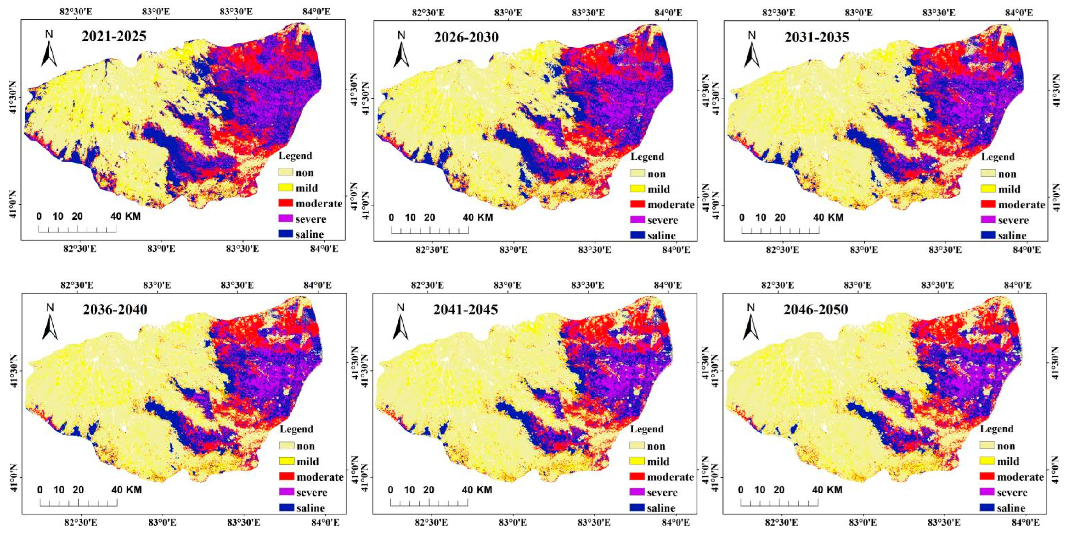
3.5. Soil Salinity Predictions for 2020–2050

In previous research, we set 2001, 2005, and 2010 as the test years. Additionally, 2005 was set as the start year, while the averaged variables from 2005 to 2010 were used to generate a suitability atlas, with 2015 set as the target year. The test results were reasonable, with a kappa coefficient of 0.6464 and overall accuracy of 73.16%. Then, we set 2015 as the start year, used the averaged variables of 2010–2015 to generate the suitability atlas, and set 2020 as the target year, resulting in a kappa coefficient of 0.6613 and overall accuracy of 74.52%. This accuracy was similar to or slightly lower than that of other studies. For example, some scholars have simulated land use in China with the future land use simulation (FLUS) model, and the overall kappa was 0.67, similar to that in our study [72]. Then, they used the FLUS, CLUE-S, ANN-CA, and Logistic-CA models to simulate land types in the Pearl River Delta, and the Kappa coefficients were 0.7963, 0.7582, 0.7332, and 0.7100, respectively. Moreover, Fu et al. [25] predicted the land types of Mianzhu City using the CA–Markov model, with a kappa value was of 0.91. Gao et al. [59] simulated the land types in the Baiyangdian Basin in 2035 using the CA–Markov model, with a kappa value of 0.8674. Chen et al. [73] predicted land use in the Kubuqi Desert in 2025–2035 using the CA–Markov model, with a kappa value of 0.79. These results may be due to the evolution of soil salinity, which presents noticeable differences for different land use types. Additionally, one salinity type may correspond to various land use types; for example, the non-saline soil may correspond to cultivated land, grassland, and forestland, whereas mildly saline soil mainly corresponds to cultivated land, and saline soil mainly corresponds to desert and low-altitude areas. Therefore, as previously demonstrated, the evolution process of the saline soil type is highly complicated, and data from only two different years should not be used to predict future trends. Therefore, we used data from 5-year intervals, with 2006–2010 as the starting range, and used the averaged variables from 2011 to 2015 to generate the suitability atlas and 2016–2020 as the target years. Then, these data were used to construct the CA–Markov model, whereas the trained model was used to predict the soil salinity types from 2016 to 2020. The kappa index of the prediction result was 0.6736 (Figure 10), overall accuracy was 75.05%, which was higher than the single-year prediction (kappa = 0.6613), and the area ratio error as within 5% (

Table 5. Comparison of prediction and observation results for 2016–2020 (unit: km²).

Salinity Type	Observed	Proportion (%)	Prediction	Proportion (%)
Non	3518.63	37.08	3221.25	33.94
Mild	717.79	7.56	867.56	9.14
Moderate	1086.22	11.45	1388.31	14.63
Severe	1230.47	12.97	1479.97	15.60
Saline	2936.74	30.95	2532.75	26.69

). Furthermore, the predicted results, presented in Figure 11, were more consistent with the actual results. However, in the inner-oasis region and east of the region, predictions of some of the moderate and saline soil areas were not very reasonable. These results indicate that the overall accuracy of the prediction was reasonable (Kappa coefficients were between 0.6464 and 0.6736, the overall accuracy was between 73.16 and 75.05%, and the area ratio error was within 5%). However, compared to many other studies on land use prediction mentioned here, this accuracy was similar to or slightly lower than that of these studies. We must continuously verify our prediction accuracy based on the measured results in the future.

Based on our analyses, we set the salinization type map corresponding to the average SSC from 2016 to 2020 as the start year, used the average variables for 2016–2020 to generate the suitability evaluation atlas, and predicted the soil salinity type from 2020 to 2050. The prediction results showed that the saline soil areas decreased while the non-saline and mildly saline soil areas increased (Figure 11). For example, non-saline areas increased from 3777.70 km² (occupying 39.81%) from 2021 to 2025 to 5421.65 km² (occupying 57.13%) from 2046 to 2050, whereas the area of saline soil decreased from 2173.24 km² (occupying 22.9%) from 2021 to 2025 to 1167.97 km² (occupying 12.31%) from 2046 to 2050 (

Table 6. Area and proportion of soil salinization from 2020 to 2050 (unit: km²).

Year	Non	Proportion (%)	Mild	Proportion (%)	Moderate	Proportion (%)	Severe	Proportion (%)	Saline	Proportion (%)
2021–2025	3777.70	39.81	1036.43	10.92	1316.02	13.87	1186.48	12.50	2173.24	22.90
2026–2030	4291.33	45.22	1016.13	10.71	1241.82	13.09	1067.58	11.25	1873.01	19.74
2031–2035	4686.89	49.39	1009.66	10.64	1187.50	12.51	972.06	10.24	1633.74	17.22
2036–2040	4993.75	52.62	1009.32	10.64	1148.23	12.10	895.92	9.44	1442.63	15.20
2041–2045	5233.47	55.15	1011.35	10.66	1119.34	11.80	835.75	8.81	1289.94	13.59
2046–2050	5421.65	57.13	1014.12	10.69	1097.75	11.57	788.37	8.31	1167.97	12.31

).

In the future, the overall spatial pattern from 2026 to 2030 is predicted to be similar to historical trends. The non-saline and mildly saline areas were dominant in the oasis area, whereas the severely saline soil was mostly distributed in the eastern and southern parts of the desert region. Moreover, the non-saline areas were mostly converted to mildly saline areas, with an extent of 162.47 km², which was mostly located around mildly saline areas. Additionally, the mildly saline soil was mostly converted to non-saline soil, with an area of 168.09 km². The moderately saline soil was mostly converted to non-saline and mildly saline areas, with an extent of 343.38 and 168.19 km², respectively, and they were distributed throughout the entire research area. The severely saline soil was mostly converted to non-saline and moderate salinization, with an area of 206.18 and 188.51 km², respectively, and they were largely distributed in the eastern and southern parts of the oasis region. The saline soil area was mostly converted to non-saline, moderately saline, and severely saline areas, with an extent of 357.17, 303.50, and 334.38 km², respectively; they were mostly distributed in the eastern and southern parts of the research area.

From 2046 to 2050, the overall spatial pattern is predicted to be similar to the historical trend. The non-saline soil will expand annually to the entire study area, especially in the northeastern and eastern parts of the study area, where the transformation will be highly significant. Throughout the entire region, from 2046 to 2050, numerous mild, moderate, severe, and saline soil areas were converted to non-saline soil areas, with areas of 188.33, 485.47, 370.85, and 1044.13 km², respectively. In the inner oasis region, most of the moderately saline soil was converted to mildly saline soil. In contrast, most moderate and saline soils in the eastern part of the oasis, northeastern study area, and southern area near the Tarim River were converted to non-saline soils. However, 125.71 km² of non-saline soil was converted to mildly saline soil, mainly in agricultural areas. Further, the mild area was converted to moderate, the moderate area was converted to severe, and the severe area was converted to saline, with areas of 54.00, 25.88, and 62.93 km², respectively. Thus, effective control measures should be implemented in advance for areas with severe salinization. Hassani et al. [23] predicted the primary soil salinity under different climate change scenarios in arid areas (RCP4.5, RCP8.5, SSP2-4.5, and SSP-8.5) and reported that soil salinization in many countries and regions showed a downward trend. Thus, at the macro level, our study results are similar to those of Hassani et al. [23].

3.6. Limitations

We acknowledge that there were some limitations in this study. First, we simply put together soil samples from different months over time, which may have had a slight impact on the results. Further precise evaluation work is needed in the future. Second, there are many factors affecting soil salinization that are difficult to consider comprehensively, such as terrain attributes, land use, soil properties, climatic factors, vegetation, and hydrothermal conditions. Finally, the prediction accuracy of soil salinization must be further improved.

4. Conclusions

Considering the extreme complexity of the soil salinization process, we attempted to propose a research framework based on the CA–Markov model to predict the spatiotemporal changes in soil salinization, achieving reasonable prediction accuracy through a relatively simple and highly operational prediction process, which is different from previous simulation studies of pure land use change. This study attempted to couple the mean values of soil salinization environmental variables across multiple years to create a suitable dataset for predicting soil salinization, which slightly improves the prediction accuracy. Soil salinization was estimated using several ML methods (RF, GBDT, LightGBM, and XGBoost), and the results showed that the LightGBM algorithm had the highest precision (MAE = 9.20, RMSE = 11.88, R² = 0.73, and RPIQ = 3.08). Then, the soil salinization types were predicted from 2020 to 2050 using the CA–Markov model. Overall, moderate or severe saline soils were located in the eastern and southern parts of the Werigan–Kuqa River Delta Oasis, while mildly saline or non-saline areas were located in the inner oasis area. An overall decreasing trend was observed over the last 21 years (2001–2021) at a rate of 4.28 g/kg·10 a⁻¹. Additionally, the area with increased salinity was mainly distributed in the eastern and southern parts of the study region. The primary soil salinity change was from heavy to light salinization. Additionally, the relatively notable factors that affected soil salinity were the temperature and vegetation-related and soil-related variables. The GDVI (51%), Bio (30%), and TVDI (27%) variables had the strongest influence. Overall, the CA–Markov model had a reasonable prediction result (kappa = 0.6736). In the future, from 2046 to 2050, the salinized soil area will decrease, while non-saline and mildly saline areas will increase. However, the mild area will be converted to moderate, the moderate area will be converted to severe, and the severe area will be converted to saline soil over areas of 54.00, 25.88, and 62.93 km², respectively. Therefore, effective control measures should be put in place for areas with increased salinization. The annual decreasing salt content implies that significant achievements have been made in local salinization control. In the future, the severity of soil salinization may be reduced based on the comprehensive impact of reclaiming wasteland, salinization control, climate change, and salinization policies. Furthermore, for the predicted future results (2025–2050), due to the lack of measured data, we were unable to accurately obtain the accuracy evaluation results for the future period. However, we will continuously verify our prediction accuracy based on future measured results.

References

1. Khan, N.M.; Rastoskuev, V.V.; Shalina, E.V.; Sato, Y. Mapping salt-affected soils using remote sensing indicators—A simple approach with the use of GIS IDRISI. In Proceedings of the 22nd Asian Conference on Remote Sensing, Singapore, 5–9 November 2001. [Google Scholar]
2. Moreau, S.S. Application of remote sensing and GIS to the mapping of saline\sodic soils and evaluation of codification risks in the Province of Villarreal, central Altiplano, Bolivia. In Proceedings of the 4th International Symposium on High Mountain Remote Sensing Cartography, Berlin, Germany, 22–26 July 1996; pp. 19–29. [Google Scholar]
3. Dwivedi, R.S.; Sreenivas, K. Image transforms as a tool for the study of soil salinity and alkalinity dynamics. Int. J. Remote Sens. 1998, 19, 605–619. [Google Scholar] [CrossRef]
4. Zhang, T.-T.; Qi, J.-G.; Gao, Y.; Ouyang, Z.-T.; Zeng, S.-L.; Zhao, B. Detecting soil salinity with MODIS time series VI data. Ecol. Indic. 2015, 52, 480–489. [Google Scholar] [CrossRef]
5. Singh, A. Soil salinization management for sustainable development: A review. J. Environ. Manag. 2020, 277, 111383. [Google Scholar] [CrossRef] [PubMed]
6. McBratney, A.B.; Santos, M.M.; Minasny, B. On digital soil mapping. Geoderma 2003, 117, 3–52. [Google Scholar] [CrossRef]
7. Minasny, B.; McBratney, A. Digital soil mapping: A brief history and some lessons. Geoderma 2016, 264, 301–311. [Google Scholar] [CrossRef]
8. Beguin, J.; Fuglstad, G.-A.; Mansuy, N.; Paré, D. Predicting soil properties in the Canadian boreal forest with limited data: Comparison of spatial and non-spatial statistical approaches. Geoderma 2017, 306, 195–205. [Google Scholar] [CrossRef]
9. Padarian, J.; Minasny, B.; McBratney, A.B. Machine learning and soil sciences: A review aided by machine learning tools. SOIL 2020, 6, 35–52. [Google Scholar] [CrossRef]
10. Taghizadeh-Mehrjardi, R.; Schmidt, K.; Toomanian, N.; Heung, B.; Behrens, T.; Mosavi, A.; Band, S.S.; Amirian-Chakan, A.; Fathabadi, A.; Scholten, T. Improving the spatial prediction of soil salinity in arid regions using wavelet transformation and support vector regression models. Geoderma 2021, 383, 114793. [Google Scholar] [CrossRef]
11. Lui, T.C.; Gregory, D.D.; Anderson, M.; Lee, W.-S.; Cowling, S.A. Applying machine learning methods to predict geology using soil sample geochemistry. Appl. Comput. Geosci. 2022, 16, 100094. [Google Scholar] [CrossRef]
12. Liu, J.; Yang, K.; Tariq, A.; Lu, L.; Soufan, W.; El Sabagh, A. Interaction of climate, topography and soil properties with cropland and cropping pattern using remote sensing data and machine learning methods. Egypt. J. Remote Sens. Space Sci. 2023, 26, 415–426. [Google Scholar] [CrossRef]
13. Gorji, T.; Sertel, E.; Tanik, A. Monitoring soil salinity via remote sensing technology under data scarce conditions: A case study from Turkey. Ecol. Indic. 2017, 74, 384–391. [Google Scholar] [CrossRef]
14. Allbed, A.; Kumar, L. Soil salinity mapping and monitoring in arid and semi-arid regions using remote sensing technology: A review. Adv. Remote Sens. 2013, 2, 373–385. [Google Scholar] [CrossRef]
15. Metternicht, G.I.; Zinck, J.A. Remote sensing of soil salinity: Potentials and constraints. Remote Sens. Environ. 2003, 85, 1–20. [Google Scholar] [CrossRef]
16. Qiao, M.; Zhou, S.; Lu, L.; Yan, J.; Song, P.; Xu, W. Causes and spatial-temporal changes of soil salinization in Weigan River Basin, Xinjiang. Prog. Geogr. 2012, 31, 904–910. [Google Scholar]
17. Bian, L.; Wang, J.; Liu, J.; Han, B. Spatiotemporal Changes of Soil Salinization in the Yellow River Delta of China from 2015 to 2019. Sustainability 2021, 13, 822. [Google Scholar] [CrossRef]
18. Alnaimy, M.A.; Elrys, A.S.; Zelenakova, M.; Pietrucha-Urbanik, K.; Merwad, A.-R.M. The Vital Roles of Parent Material in Driving Soil Substrates and Heavy Metals Availability in Arid Alkaline Regions: A Case Study from Egypt. Water 2023, 15, 2481. [Google Scholar] [CrossRef]
19. Yin, X.; Feng, Q.; Li, Y.; Deo, R.; Liu, W.; Zhu, M.; Zheng, X.; Liu, R. An interplay of soil salinization and groundwater deg-radation threatening coexistence of oasis-desert ecosystems. Sci. Total Environ. 2022, 806, 150599. [Google Scholar] [CrossRef]
20. Li, Y.; Wang, C.; Wright, A.; Liu, H.; Zhang, H.; Zong, Y. Combination of GF-2 high spatial resolution imagery and land surface factors for predicting soil salinity of muddy coasts. Catena 2021, 202, 105304. [Google Scholar] [CrossRef]
21. Corwin, D.L. Climate change impacts on soil salinity in agricultural areas. Eur. J. Soil Sci. 2021, 72, 842–862. [Google Scholar] [CrossRef]
22. Schofield, R.V.; Kirkby, M.J. Application of salinization indicators and initial development of potential global soil salinization scenario under climatic change. Glob. Biogeochem. Cycles 2003, 17. [Google Scholar] [CrossRef]
23. Hassani, A.; Azapagic, A.; Shokri, N. Global predictions of primary soil salinization under changing climate in the 21st century. Nat. Commun. 2021, 12, 6663. [Google Scholar] [CrossRef] [PubMed]
24. Zhang, Y.; Chang, X.; Liu, Y.; Lu, Y.; Wang, Y.; Liu, Y. Urban expansion simulation under constraint of multiple ecosystem services (MESs) based on cellular automata (CA)-Markov model: Scenario analysis and policy implications. Land Use Policy 2021, 108, 105667. [Google Scholar] [CrossRef]
25. Fu, F.; Deng, S.; Wu, D.; Liu, W.; Bai, Z. Research on the spatiotemporal evolution of land use landscape pattern in a county area based on CA-Markov model. Sustain. Cities Soc. 2022, 80, 103760. [Google Scholar] [CrossRef]
26. Wang, L.; Hu, P.; Zheng, H.; Liu, Y.; Cao, X.; Hellwich, O.; Liu, T.; Luo, G.; Bao, A.; Chen, X. Integrative modeling of heterogeneous soil salinity using sparse ground samples and remote sensing images. Geoderma 2023, 430, 116321. [Google Scholar] [CrossRef]
27. Li, X.; Yang, J.; Liu, M.; Liu, G.; Mei, Y. Spatio-temporal changes of soil salinity in arid areas of south Xinjiang using electromagnetic induction. J. Integr. Agric. 2012, 11, 1365–1376. [Google Scholar] [CrossRef]
28. Gorelick, N.; Hancher, M.; Dixon, M.; Ilyushchenko, S.; Thau, D.; Moore, R. Google Earth Engine: Planetary-scale geospatial analysis for everyone. Remote Sens. Environ. 2017, 202, 18–27. [Google Scholar] [CrossRef]
29. Wang, F.; Yang, S.; Wei, Y.; Shi, Q.; Ding, J. Characterizing soil salinity at multiple depth using electromagnetic induction and remote sensing data with random forests: A case study in Tarim River Basin of southern Xinjiang, China. Sci. Total Environ. 2021, 754, 142030. [Google Scholar] [CrossRef] [PubMed]
30. Taghizadeh-Mehrjardi, R.; Minasny, B.; Sarmadian, F.; Malone, B. Digital mapping of soil salinity in Ardakan region, central Iran. Geoderma 2014, 213, 15–28. [Google Scholar] [CrossRef]
31. Sandholt, I.; Rasmussen, K.; Andersen, J. A simple interpretation of the surface temperature/vegetation index space for assessment of surface moisture status. Remote Sens. Environ. 2002, 79, 213–224. [Google Scholar] [CrossRef]
32. Wang, F.; Ding, J.; Wei, Y.; Zhou, Q.; Yang, X.; Wang, Q. Sensitivity analysis of soil salinity and Vegetation indices to detect soil salinity variation by using Landsat series images: Application in different oases in Xinjiang, China. Acta Ecol. 2017, 37, 5007–5022. [Google Scholar]
33. Batjes, N.H.; Ribeiro, E.; van Oostrum, A. Standardised soil profile data to support global mapping and modelling (WoSIS snapshot 2019). Earth Syst. Sci. Data 2020, 12, 299–320. [Google Scholar] [CrossRef]
34. Cheng, X.; Zhou, Z.; Li, W.; Shangguan, D.; Wang, X.; Zhang, X.; Hao, J.; Lin, Q. Monitoring drought situation and analyzing influencing factors in Central Asia using MODIS data. Trans. Chin. Soc. Agric. Eng. (Trans. CSAE) 2022, 38, 128–137. [Google Scholar]
35. He, B.; Ding, J.; Liu, B.; Wang, J. Spatiotemporal variation of soil salinization in Weigan-Kuqa River Delta Oasis. Sci. Silvae Sin. 2019, 55, 185–196. [Google Scholar]
36. Krishnan, S.; Indu, J. Assessing the potential of temperature/vegetation index space to infer soil moisture over Ganga Basin. J. Hydrol. 2023, 621, 129611. [Google Scholar] [CrossRef]
37. Li, Y.; Chang, C.; Wang, Z.; Zhao, G. Remote sensing prediction and characteristic analysis of cultivated land salinization in different seasons and multiple soil layers in the coastal area. Int. J. Appl. Earth Obs. Geoinf. 2022, 111, 102838. [Google Scholar] [CrossRef]
38. Guo, X.; Gui, X.; Xiong, H.; Hu, X.; Li, Y.; Cui, H.; Qiu, Y.; Ma, C. Critical role of climate factors for groundwater potential mapping in arid regions: Insights from random forest, XGBoost, and LightGBM algorithms. J. Hydrol. 2023, 621, 129599. [Google Scholar] [CrossRef]
39. Kaplan, G.; Gašparović, M.; Alqasemi, A.S.; Aldhaheri, A.; Abuelgasim, A.; Ibrahim, M. Soil salinity prediction using Machine Learning and Sentinel-2 Remote Sensing Data in Hyper-Arid areas. Phys. Chem. Earth Parts A/B/C 2023, 130, 103400. [Google Scholar] [CrossRef]
40. He, Y.; Zhang, Z.; Xiang, R.; Ding, B.; Du, R.; Yin, H.; Chen, Y.; Ba, Y. Monitoring salinity in bare soil based on Sentinel-1/2 image fusion and machine learning. Infrared Phys. Technol. 2023, 131, 104656. [Google Scholar] [CrossRef]
41. Fathizad, H.; Ardakani, M.A.H.; Sodaiezadeh, H.; Kerry, R.; Taghizadeh-Mehrjardi, R. Investigation of the spatial and temporal variation of soil salinity using random forests in the central desert of Iran. Geoderma 2020, 365, 114233. [Google Scholar] [CrossRef]
42. Das, A.; Bhattacharya, B.K.; Setia, R.; Jayasree, G.; Das, B.S. A novel method for detecting soil salinity using AVIRIS-NG imaging spectroscopy and ensemble machine learning. ISPRS J. Photogramm. Remote Sens. 2023, 200, 191–212. [Google Scholar] [CrossRef]
43. Tariq, A.; Yan, J.; Mumtaz, F. Land change modeler and CA-Markov chain analysis for land use land cover change using satellite data of Peshawar, Pakistan. Phys. Chem. Earth Parts A/B/C 2022, 128, 103286. [Google Scholar] [CrossRef]
44. Heung, B.; Ho, H.C.; Zhang, J.; Knudby, A.; Bulmer, C.E.; Schmidt, M.G. An overview and comparison of machine-learning techniques for classification purposes in digital soil mapping. Geoderma 2016, 265, 62–77. [Google Scholar] [CrossRef]
45. Hong, Y.; Shen, R.; Cheng, H.; Chen, Y.; Zhang, Y.; Liu, Y.; Zhou, M.; Yu, L.; Liu, Y.; Liu, Y. Estimating lead and zinc concentrations in peri-urban agricultural soils through reflectance spectroscopy: Effects of fractional-order derivative and random forest. Sci. Total Environ. 2018, 651 Pt 2, 1969–1982. [Google Scholar] [CrossRef]
46. Dewage, S.N.S.P.; Minasny, B.; Malone, B. Disaggregating a regional-extent digital soil map using Bayesian area-to-point regression kriging for farm-scale soil carbon assessment. SOIL 2020, 6, 359–369. [Google Scholar] [CrossRef]
47. Kursa, M.B.; Rudnicki, W.R. Feature Selection with the Boruta Package. J. Stat. Softw. 2010, 36, 1–13. [Google Scholar] [CrossRef]
48. Friedman, J.H. Greedy function approximation: A gradient boosting machine. Ann. Stat. 2001, 29, 1189–1232. [Google Scholar] [CrossRef]
49. Meng, R. Research on Water Depth Inversion Method Based on Remote Sensing Image. Master’s Thesis, Shanghai Ocean University, Shanghai, China, 2022. [Google Scholar]
50. Ke, R.; Wu, S.; Ke, W. A spatial-temporal model for identifying tidal shared-bicycle stops and bicycle sharing demand pre-diction based on KNN-LightGBM. J. Geoinf. Sci. 2023, 25, 741–753. [Google Scholar]
51. Ke, G.; Meng, Q.; Finley, T.; Wang, T.; Chen, W.; Ma, W.; Ye, Q.; Liu, T. LightGBM: A highly efficient gradient boosting decision tree. Adv. Neural Inf. Process. Syst. 2017, 30. [Google Scholar]
52. Xiao, C.; Ji, Q.; Chen, J.; Zhang, F.; Li, Y.; Fan, J.; Hou, X.; Yan, F.; Wang, H. Prediction of soil salinity parameters using machine learning models in an arid region of Northwest China. Comput. Electron. Agric. 2023, 204, 107512. [Google Scholar] [CrossRef]
53. Chen, T.; Guestrin, C. XGBoost: A scalable tree boosting system. In Proceedings of the KDD ’16: The 22nd ACM SIGKDD International Conference on Knowledge Discovery and Data Mining, San Francisco, CA, USA, 13–17 August 2016; pp. 785–794. [Google Scholar]
54. Li, Y.; Peng, D.; Yuan, Y. Airborne LiDAR data inversion of forest aboveground biomass using XGBoost algorithm. J. Northeast. For. Univ. 2023, 51, 106–112. [Google Scholar]
55. Huang, Z.; Shen, J.; Jian, W.; Fan, X.; Nie, W. Displacement prediction of rainfall-induced step-like landslide based on XGBoost model. J. Nat. Disasters 2023, 32, 217–226. [Google Scholar]
56. Yang, G.; Liu, Y.; Wu, Z. Analysis and simulation of land-use temporal and spatial pattern based on CA-Markov model. Geomat. Inf. Sci. Wuhan Univ. 2007, 32, 414–418. [Google Scholar]
57. Yang, J.; Xie, P.; Xi, J.; Ge, Q.; Li, X.; Ma, Z. LUCC simulation based on the cellular automata simulation: A case study of Dalian Economic and Technological Development Zone. Acta Geogr. Sin. 2015, 70, 461–475. [Google Scholar]
58. Qian, Y.; Xing, W.; Guan, X.; Yang, T.; Wu, H. Coupling cellular automata with area partitioning and spatiotemporal convolution for dynamic land use change simulation. Sci. Total Environ. 2020, 722, 137738. [Google Scholar] [CrossRef]
59. Gao, X.; Yang, L.; Li, C.; Song, Z.; Wang, J. Land use change and ecosystem service value measurement in Baiyangdian Basin under the simulated multiple scenarios. Acta Ecol. Sin. 2021, 41, 7974–7988. [Google Scholar]
60. He, Y.; Fan, G.; Zhang, X.; Li, Z.; Gao, D. Vegetation phenological variation and its response to climate changes in Zhejiang province. J. Nat. Resour. 2013, 28, 220–233. [Google Scholar]
61. Tursun, H.; Turangul, H. soil salinization types in typical oasis in Northern Taklamakan Basin. Heilongjiang Agric. Sci. 2017, 4, 24–30. [Google Scholar]
62. Qiao, M.; Zhou, S.; Lu, L.; Yan, J.; Li, H. Temporal and spatial changes of soil salinization and improved countermeasures of Tarim Basin Irrigation District in recent 25 a. Arid. Land Geogr. 2011, 34, 604–613. [Google Scholar]
63. Qiao, M.; Tian, C.; Wang, X. Soil Salinization and Its Improvement and Control Model in Irrigation Areas of Xinjiang; Xinjiang Science and Technology Publishing House: Urumqi, China, 2008; pp. 1–25. [Google Scholar]
64. Jiao, R.; Bu, D.; Zhang, T.; Shao, Y.; Chen, L.; Shui, Y. Evaluation of soil nutrient status in Alar cotton planting area of Xinjiang. J. Shihezi Univ. 2023, 41, 160–167. [Google Scholar]
65. Zhao, Z.; Zhang, H.; Huang, J.; Li, F.; Yu, Q. Dynamic change of water and salt and their coupling relationships in Weigan River Irrigation District. J. Arid. Land Resour. Environ. 2008, 22, 142–146. [Google Scholar]
66. Wang, X.; Gao, Q.; Lu, Q.; Li, B. Salt-water balance and dry drainage desalting in Hetao irrigating area, Inner Mongolia. Sci. Geogr. Sin. 2006, 26, 455–460. [Google Scholar]
67. Zhang, X.; Yang, D.; Liu, Y. Emergy-based sustainability and sensitivity analysis of oasis cropping system: A case study in Weigan River Basin. Acta Ecol. Sin. 2009, 29, 6068–6076. [Google Scholar]
68. Akramkhanov, A.; Martius, C.; Park, S.; Hendrickx, J. Environmental factors of spatial distribution of soil salinity on flat irrigated terrain. Geoderma 2011, 163, 55–62. [Google Scholar] [CrossRef]
69. Moore, I.D.; Grayson, R.B.; Ladson, A.R. Digital terrain modelling: A review of hydrological, geomorphological, and biological applications. Hydrol. Process 1991, 5, 3–30. [Google Scholar] [CrossRef]
70. Jafari, A.; Finke, P.A.; Wauw, J.V.; Ayoubi, S.; Khademi, H. Spatial prediction of USDA- great soil groups in the arid Zarand region, Iran: Comparing logistic regression approaches to predict diagnostic horizons and soil types. Eur. J. Soil Sci. 2012, 63, 284–298. [Google Scholar] [CrossRef]
71. Ge, X.; Ding, J.; Teng, D.; Wang, J.; Huo, T.; Jin, X.; Wang, J.; He, B.; Han, L. Updated soil salinity with fine spatial resolution and high accuracy: The synergy of Sentinel-2 MSI, environmental covariates and hybrid machine learning approaches. CATENA 2022, 212, 106054. [Google Scholar] [CrossRef]
72. Liu, X.; Liang, X.; Li, X.; Xu, X.; Ou, J.; Chen, Y.; Li, S.; Wang, S.; Pei, F. A future land use simulation model (FLUS) for simulating multiple land use scenarios by coupling human and natural effects. Landsc. Urban Plan. 2017, 168, 94–116. [Google Scholar] [CrossRef]
73. Chen, H.; Gao, Y.; Dang, X. Prediction of land use change in Kubuqi Desert based on CA—Markov model. J. Inn. Mong. For. Sci. Technol. 2022, 48, 18–22+34. [Google Scholar]
Figure 1. Location and sample distribution map of the study area: (a) location of the study area, (b) specific sampling locations, and (c) soil type map (ARb: Cambic Arenosols; ARh: Haplic Arenosols; ATa: Aric Anthrosols; ATc: Cumulic Anthrosols; CMc: Calcaric Cambisols; FLc: Calcaric Fluvisols; FLs: Salic Fluvisols; GLe: Eutric Gleysols; GLm: Mollic Gleysols; GYk: Calcic Gypsisols; PHc: Calcaric Phaeozems; PHg: Gleyic Phaeozems; SCg: Gleyic Solonchaks; SCh: Haplic Solonchaks; SCk: Calcic Solonchaks; SCm: Mollic Solonchaks; SCy: Gypsic Solonchaks; VRk: Calcic Vertisols; and WR: Inland water).
Sustainability 15 13996 g001
Figure 2. Pearson correlation matrix analysis of different indices. Note: Panels (ad) refer to the correlation matrix composed of groups of 24 variables (each group includes electrical conductivity).
Sustainability 15 13996 g002
Figure 3. Framework for predicting soil salinity in this study.
Sustainability 15 13996 g003
Figure 4. Spatial distribution of SSC from 2001 to 2021. (note: non, non-saline; mild, mildly saline; moderate, moderately saline; severe, severely saline; and saline, saline soil).
Sustainability 15 13996 g004aSustainability 15 13996 g004b
Figure 5. Change in the SSC in the Weiku Oasis from 2001 to 2021.
Sustainability 15 13996 g005
Figure 6. Trend diagram of the soil salinity content for the different soil salinity types: (a) non−saline, (b) mildly saline, (c) moderately saline, (d) severely saline, and (e) saline soil.
Sustainability 15 13996 g006
Figure 7. Trend of the SSC/(g/kg·10 a−1).
Sustainability 15 13996 g007
Figure 8. Spatial distribution of soil salinization type changes from 2001 to 2021. (Note: Non, non-saline; Mild, mildly saline; Mod, moderately saline; Sev, severely saline; and Sal, saline soil.)
Sustainability 15 13996 g008
Figure 9. Relative significance of the auxiliary data. Abbreviations: GDVI, generalized difference vegetation index; Bio9, the ninth bioclimatic variables; TVDI, temperature vegetation drought index; SOC_60_100, Soil organic carbon at a depth of 60–100 cm; SOCS, soil organic carbon stock (SOCS); TWI, topographic wetness index; and TRI, topographic relief index.
Sustainability 15 13996 g009
Figure 10. (a) Soil salinity map for 2016–2020 and (b) simulation soil salinity map for 2016–2020. Abbreviations: non, non-saline; mild, mildly saline; moderate, moderately saline; severe, severely saline; and saline, saline soil.
Sustainability 15 13996 g010
Figure 11. Soil salinity map from 2020 to 2050. (Note: non, non–saline; mild, mildly saline; moderate, moderately saline; severe, severely saline; and saline, saline soil.)
Sustainability 15 13996 g011