Machine Learning Prediction and Optimization of Performance and Emissions Characteristics of IC Engine

Abstract

In this work, a study was conducted to investigate the effects of different biodiesel blends with hydrogen peroxide additive on the performance and emissions of an internal combustion engine under various operating parameters. A CI engine was operated with diesel, four dissimilar biodiesels, and H₂O₂ at various proportions. The biodiesel blends used were Jatropha (D60JB30A10, D60JB34A6, D60JB38A2, D60JB40), Honge (D60HB30A10, D60HB34A6, D60HB38A2, D60HB40), Simarouba (D60SB30A10, D60SB34A6, D60SB38A2, D60SB40), and Neem (D60NB30A10, D60NB34A6, D60NB38A2, D60NB40). The engine was tested at different injection operating pressures (200, 205, and 210 bar), a speed of 1500 rpm, and a CR of 17.5:1. From the experiments conducted, it was highlighted that, under specific conditions, i.e., with an injection pressure of 205 bar, 80% load, a compression ratio of 17.5, an injection timing set at 230 before top dead center, and an engine speed of 1500 rpm, the biodiesel blends D60JB30A10, D60HB30A10, D60SB30A10, and D60NB30A10 achieved the highest brake thermal efficiencies of 24%, 23.9675%, 23.935%, and 23.9025%, respectively. Notably, the blend D60JB30A10 stood out with the highest brake thermal efficiency of 24% among these tested blends. Similarly, when evaluating emissions under the same operational conditions, the D60JB30A10 blend exhibited the lowest emissions levels: CO (0.16% Vol), CO₂ (7.8% Vol), HC (59 PPM), and Smoke (60 HSU), while NOx (720 PPM) emissions showed a relative increase with higher concentrations of the hydrogen-based additive. The D60HB30A10, D60SB30A10, and D60NB30A10 blends showed higher emissions in comparison. Additionally, the study suggests that machine learning techniques can be employed to predict engine performance and emission characteristics, thereby cutting down on time and costs associated with traditional engine trials. Specifically, machine learning methods, like XG Boost, random forest regressor, decision tree regressor, and linear regression, were utilized for prediction purposes. Among these techniques, the XG Boost model demonstrated highly accurate predictions, followed by the random forest regressor, decision tree regressor, and linear regression models. The accuracy of the predictions for XG Boost model was assessed through evaluation metrics such as R2-Score (0.999), Root Mean Squared Error (0.540), Mean Squared Error (0.248), and Mean Absolute Error (0.292), which allowed for a thorough analysis of the algorithm’s performance compared to actual values.

1. Introduction

Biodiesel fuels are derived from vegetable oil or animal fat resources through a process called transesterification, resulting in mono-alkyl esters of long-chain fatty acids. While biodiesel offers numerous benefits as a substitute for fossil diesel, its main drawback lies in the elevated levels of nitrogen oxides (NOx) emissions [1,2,3,4,5,6]. The rise in nitrogen oxides (NOx) emissions linked to biodiesel, commonly referred to as the biodiesel-NOx penalty, can be attributed to several factors. These factors include the advancement of injection timing [7], which leads to increased NOx formation. Additionally, biodiesel combustion tends to generate higher flame temperatures [8], contributing to higher NOx production. Moreover, differences in fuel properties, such as biodiesel’s higher density, lower energy content, lower volatility, and higher iodine number, also play a role in the increased NOx emissions. These various factors collectively contribute to the observed biodiesel-NOx penalty [9], as well as a faster burn rate due to the presence of oxygen bound in the fuel [10]. On the other hand, it has been observed that biodiesel fuels have the potential to significantly reduce soot emissions due to the absence of sulfur and aromatics, as well as the presence of fuel-bound oxygen [9]. Experiments have been conducted by using grapeseed biodiesel as alternative fuel and hydrogen inducted as oxygenator, from experimental results it was observed that the addition of hydrogen had a positive impact on the engine’s performance, this demonstrates the potential of hydrogen as an effective additive to improve the performance of diesel engines using biofuels like grapeseed oil.

The study revealed a significant reduction in carbon-based emissions such as hydrocarbons (HC), carbon monoxide (CO), and smoke when using hydrogen fuel blends. However, it was noted that hydrogen fuel resulted in higher nitrogen oxide (NO) emissions compared to all the tested fuels. Indeed, there is a noticeable lack of literature regarding the mixture of little carbon fuels along with hydrogen and situation carbon imprison systems in order to enhance presentation and diminish tail pipe emissions in engines [11]. There are different methods to produce biodiesel [12,13,14]; among these, transesterification is most commonly used and, in this process, triglycine react with alcohol and produces methyl ester and glycerin [15,16]. This homogeneous transesterification process is not only widely adopted but also cost effective [17,18,19,20].

However, researchers have pointed out certain drawbacks associated with biodiesel combustion. These include inferior specific heat energy along with superior nitrogen oxide (NOx) emissions compared to clean petroleum diesel fuel [21,22]. Here, in response to these concerns, several methods have been explored to mitigate the issues. Some of these methods include EGR (Exhaust gas recirculation), IT (Injection time) retardation, and emulsification of biofuel blends, along with the mixing of nanoparticles to biofuel blends. These approaches aim to shrink nitrogen formation oxides and boost biodiesel’s whole energy production efficiency in automotive engines [23,24,25,26,27]. Such research endeavors to optimize the performance and environmental impact of biofuel as a substitute fuel choice. This study investigated how specific physical attributes of zinc oxide, including factors such as surface area, pore size, and dispersion, influenced the adsorptive elimination of thiophene in the presence of varying carrier gases. Alumina was used as a supporting material to enhance the dispersion of zinc oxide. Among the tested adsorbents, ZnO-550 displayed remarkable effectiveness in removing thiophene, despite having a smaller surface area and pore volume. This unexpected outcome could be attributed to larger pores that facilitated access to substantial thiophene molecules within the adsorbent. As a result, ZnO-550’s adsorption process extended beyond saturation points observed in other adsorbents. The study underscored the pivotal role of pore size in accommodating larger molecules during the adsorption process. Interestingly, the presence of hydrogen also enhanced the efficiency of sulfur compound removal, even at room temperature. The main focus of this study lies in the pursuit of developing ultra-clean fuel, which retains its paramount importance in the refining industry. This research offers valuable insights into the strategic deployment of desulfurization techniques to effectively eliminate sulfur compounds, thereby contributing to the creation of eco-friendly fuel suitable for a range of human activities. By adhering to regulations aimed at reducing sulfur content in fuel oil, the potential for producing secure and sustainable sulfur-free fuel becomes evident [28].

For a long time, the application of machine learning calculations has altogether moved forward execution over different areas, including data innovation [29], therapeutic applications [30], building [31], development [32], and different other spaces [33,34,35]. In the context of engine emission prediction, machine learning models have proven to be effective, and researchers have explored various techniques such as Artificial Neural Networks (ANN), Support Vector Regression (SVR), Decision Trees (DT), and Random Forest (RF) [36]. Comparisons between outfit learning strategies and SVM (support vector machine) utilizing the RMSE (Root mean square error) execution metric have uncovered that gathering strategies, for the most part, accomplish lower mistake rates.

Occasionally, the boosted decision tree algorithm was effectively utilized to anticipate mean compelling weight in a characteristic gas engine, with such results closely adjusted with test information and negligible error [37]. Additionally, within the case of a dual-fueled biogas–biodiesel motor, an ensemble-boosted relapse tree was utilized to foresee emanations, outflanking an ANN (artificial neural network) based on different factual parameters [38,39]. The outcomes provide experimental support and theoretical basis for the adoption of HCNG fuel on internal combustion engines, as well as the application of intelligent algorithms in the engine standardization technology field [40]. Predicting internal combustion (IC) engine variables such as the combustion phasing and period are crucial to zero-dimensional (0D) single-zone engine simulations (e.g., for the Wiebe function combustion model). The use of random forest machine learning models was examined to predict these engine ignition variables as a modality to decrease expensive engine dynamometer trials [41]. To meet the strict emission standards and attain cleaner creation of mingling fluidized bed units, it is essential to build a dynamic model of pollutants emission for creating an economical and environmentally friendly pollutant removal operation mode [42]. The main theme is to explore the fitness of several machine learning (ML) techniques including artificial neural network (ANN), adaptive neuro-fuzzy inference system (ANFIS), general regression neural network (GRNN), radial basis function (RBFN), and support vector regression (SVR) for predicting performance and exhaust emissions of the diesel engine fueled with biodiesel blends [43]. The aim is to approximate diverse air–fuel ratio motor shaft speed and fuel flow rates under the performance limits contingent on the indices of ignition efficiency and exhaust emission of the engine, a turboprop multilayer feed forward artificial neural network model [44]. This study applies machine learning tools for constrained multi-objective optimization of an HCCI (Homogeneous Charge Compression Ignition) engine. Machine learning tools have been implemented to learn the behavior of a single-cylinder engine by means of three dissimilar fuels with the HCCI strategy [45]. A machine-learning algorithm has been developed, as a simple variant of linear regression, that is capable of predicting the spray 3D topology for several fuels and ambient situations [46]. In order to deal with the huge time delay and robust nonlinear features of the ignition process, a dynamic correction prediction model considering the time delay is proposed [47].some reported characteristics in ML are shown in the

Table 1. Reported characteristics in ML analysis.

S.No	Authors	Machine Learning Algorithms	Parameter/s Used for the Prediction	Best Model for the Prediction
1	[32] Ahmad M.W. et al.	ANN and decision tree-based algorithm (random forest).	HVAC electricity consumption on hour bases.	ANN
2	[36] Ağbulut Ü. et al.	Deep learning (DL), Artificial Neural Network (ANN), Kernel Nearest Neighbor (k-NN), and Support Vector Machine (SVM)	carbon dioxide (CO), nitrogen oxide (NOx), exhaust gas temperature (EGT), brake specific fuel consumption (BSFC), and brake thermal efficiency (BTE).	Deep learning (DL),
3	[37] Liu J. et al.	ANN	carbon monoxide (CO), unburned hydrocarbons (UHC), nitrogen oxides (NOx), indicated mean effective pressure (IMEP), and indicated thermal efficiency (ITE)	ANN
4	[38] Prabhakar Sharma et al.	Boosted Regression Trees (BRT) and ANN	brake thermal efficiency (BTE), Biogas Fuel Ratio (BFR), NOx, CO, and HC.	Boosted Regression Trees (BRT)

.

This literature review focuses on efficient fuel and emerging machine learning (ML) techniques, which hold promise for predictive and optimization tasks in this field. While data-driven approaches using real-time sensor data have gained momentum, challenges like standardized datasets and real-world integration persist. Our research aims to leverage ML to predict and optimize IC Engine performance and emissions, ultimately contributing to more efficient and eco-friendly IC Engines.

The novelty of applying machine learning to predict and optimize the performance and emission characteristics of internal combustion engines lies in its data-driven approach, which contrasts with traditional physics-based models. Machine learning harnesses large datasets and algorithms to uncover complex relationships and patterns that might not be captured by conventional methods. This enables accurate real-time adaptation and optimization, accommodating a wide range of operating conditions. Moreover, machine learning’s ability to simultaneously consider multiple variables offers a holistic approach to optimization, with the potential to uncover optimal configurations that might be overlooked using traditional techniques. This novel approach has the capacity to transform engine optimization, yielding more efficient and environmentally friendly internal combustion engines. The proposed study aims to utilize machine learning algorithms to predict the performance and emission characteristics of a single-cylinder four-stroke diesel engine.

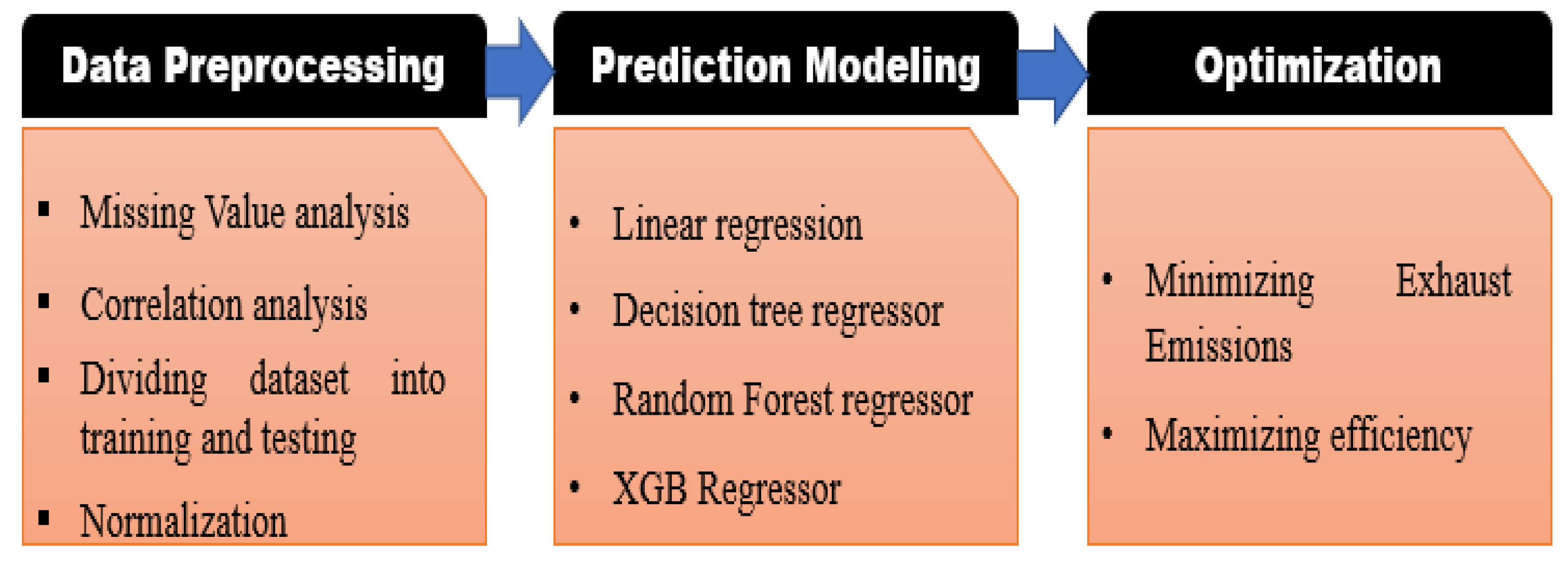
The experimentation involves different biodiesel blends and H₂O₂ as a fuel additive. Various machine learning methods, including random forest regressor, decision tree regressor, linear regression, and XG Boost are employed for making predictions. It is worth noting that random forest regressor is a bagging approach, while the remaining three are boosting methods. The optimization of hyperparameters is crucial in this work to identify the most accurate prediction model. To prevent overfitting, cross-validation techniques are implemented to ensure accurate guesses on invisible trial facts. A relative study among the algorithms using presentation assessment metrics like R2 value, RMSE, and MAE is conducted to assess their predictive capabilities accurately.

2. Material and Methods

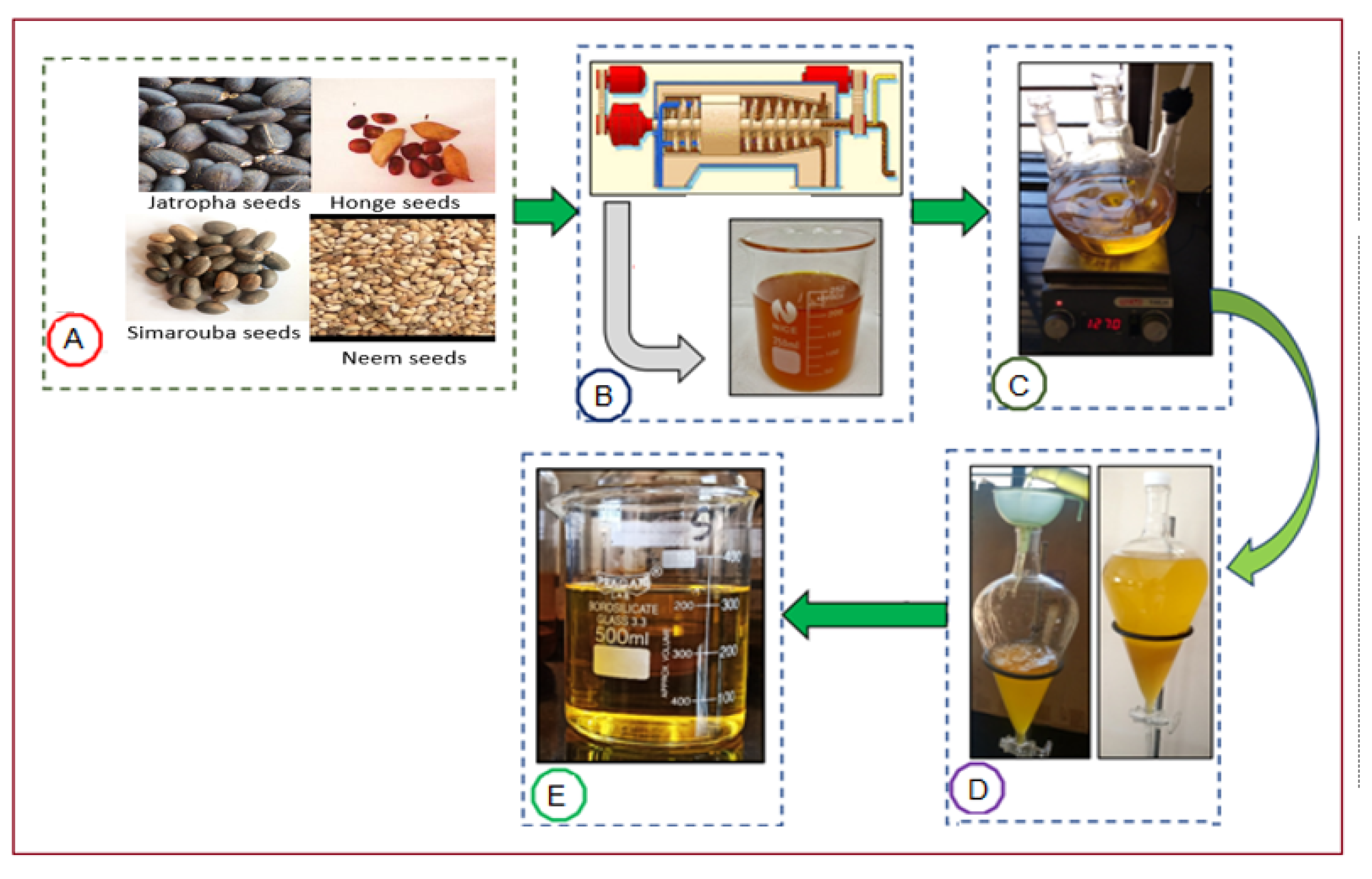
Biodiesels, including Jatropha, Honge, Simarouba, and Neem oil, are produced using a catalyzed homogeneous transesterification process. As shown in Figure 1, this process involves using Jatropha, Honge, Simarouba, and Neem oil as feedstocks. The oils undergo a series of steps, including the oil being taken out, esterification, the parting of biodiesel and glycerin, and the wash and aeriation to get clean biodiesels. H₂O₂ is used as an oxygenator in this process.

The rationale for choosing these biodiesel sources lies in their distinct properties, availability, and potential environmental benefits, contributing to our understanding of the feasibility and advantages of biodiesel utilization as an alternative to conventional fossil fuels. The sustainability of biodiesel production hinges on thoughtful decision making across its entire lifecycle. Selecting the right feedstock is crucial, as it must strike a balance between resource efficiency and minimal environmental impact. Responsible land use, efficient water management, and judicious chemical usage further contribute to sustainability. While biodiesel offers the advantage of lower carbon emissions during combustion, a holistic view of lifecycle emissions is essential. Effective waste management and pollution prevention are vital to minimize environmental harm. Moreover, biodiesel production can positively impact local economies when coupled with fair labor practices, enhancing its overall sustainability.

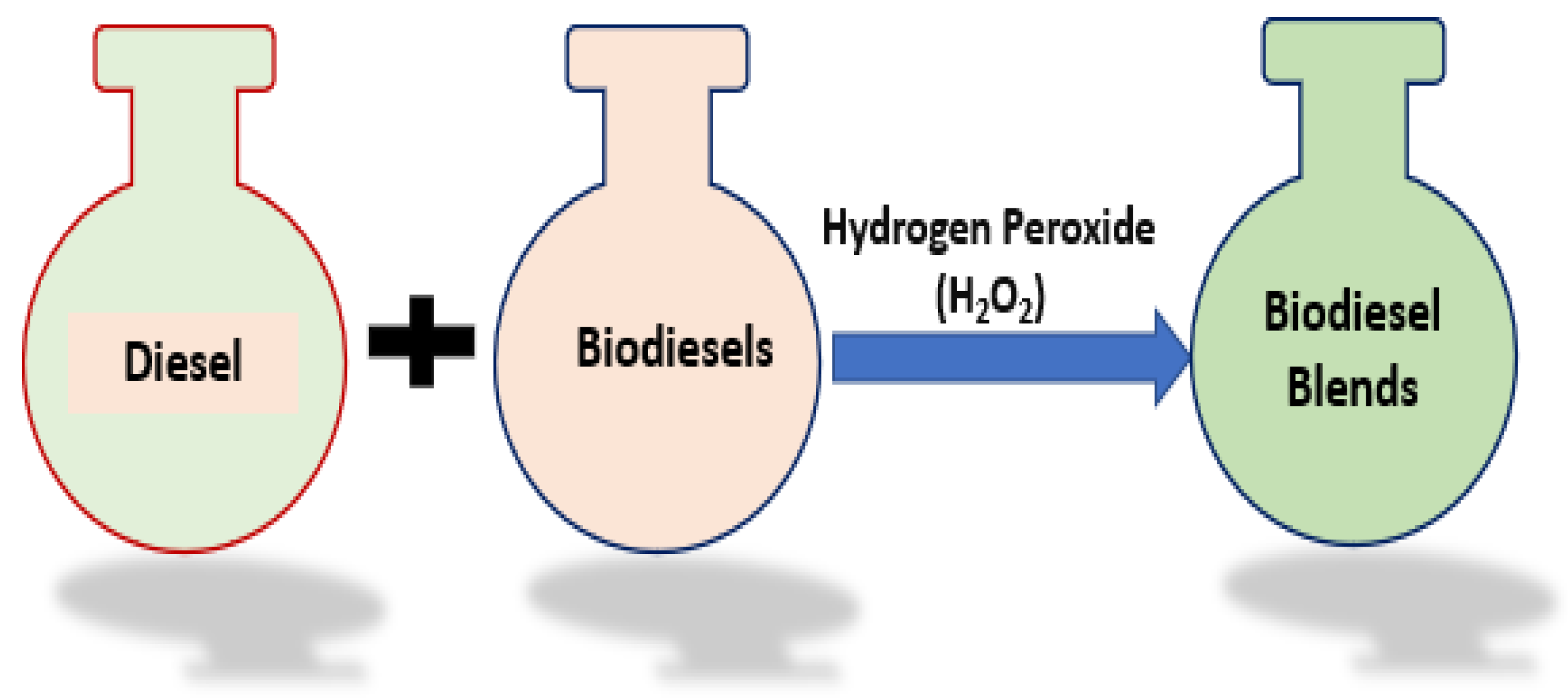
To create different biodiesel blends, combinations of the four biodiesels are prepared with varying proportions. The blends are labeled as D60B30A10 (60% diesel, 30% biofuel, and 10% H₂O₂ additive), D60B34A6 (60% diesel, 34% biofuel, and 6% H₂O₂ additive), D60B38A2 (60% diesel, 38% biofuel, and 2% H₂O₂ additive), and D60B40 (60% diesel, 40% biodiesel). The properties of these fuel blends are detailed in

Table 2. Fuel Properties Jatropha Biofuel Blends.

Fuel	Density (Kg/m3)	Viscosity (cSt) at 40 °C	Flash Point (°C)	Fire Point (°C)	Calorific Value (kJ/Kg)
Diesel	835	6.2	50	55	43,800
D60-JB30-A10	865	3.408	82	96	40,913
D60-JB34-A6	860	3.362	83	100	40,856
D60-JB38-A2	855	3.321	84	106	40,746
D60-JB40	850	3.024	90	105	42,659
Honge Biofuel Blends
D60HB30A10	863	3.308	83	97	40,824
D60HB34A6	859	3.235	84	101	40,815
D60HB38A2	853	3.183	86	106	40,753
D60JB40	846	3.002	91	104	42,649
Simarouba Biofuel Blends
D60SB30A10	858	3.589	84	98	40,789
D60SB34A6	849	3.667	86	103	40,785
D60SB38A2	843	3.683	89	108	40,753
D60SB40	835	3.788	94	109	42,649
Neem Biofuel Blends
D60NB30A10	856	3.506	89	102	40,725
D60NB34A6	839	3.563	92	105	40,515
D60NB38A2	833	3.188	98	106	40,653
D60NB40	830	3.897	99	109	42,586

.

Figure 2 provides an illustration of the mixing process, illustrating how the various biodiesel, diesel, and hydrogen peroxide additive are mixed to form the different biodiesel blends.

The determination of free fatty acid (FFA) value in biodiesel oil involves the subsequent steps:

Step 1: Fill in a burette with 50 mL of distilled water and 0.5 gm of NaOH solution.

Step 2: Fill 10 gm of the oil sample in a tapering bottle.

Step 3: Combine four droplets of the NaOH solution from the burette with the oil sample.

Step 4: Introduce a single drop of phenolphthalein indicator to the oil trial.

Step 5: Perform the titration process by slowly adding NaOH solution from the burette to the oil sample until the color of the solution changes from colorless to pink. The pink color indicates the completion of the titration process.

Step 6: Record the readings on the burette. The amount of NaOH solution used in the titration process is used to calculate the free fatty acid (FFA) value in the biodiesel sample.

Since the FFA value is found to be less than 5 for all bio-oils, the purpose of the transesterification process is to convert the bio-oil into biodiesel. The process of converting 1 L of bio-oil into pure biodiesel and preparing blends with diesel and hydrogen peroxide (H₂O₂) can be summarized as follows:

Heating the bio-oil: A volume of 1 L of bio-oil is heated to a temperature of 60 °C for a duration of two hours.

Transesterification: The heated bio-oil is stirred with a mixture consisting of 200 mL of methanol and 4.5 g of sodium hydroxide (potassium methoxide) for a duration of 30 min, this process is known as transesterification, where the bio-oil reacts with the methanol and sodium hydroxide to form biodiesel (methyl esters) and glycerol. The methanol and base (NaOH in this case) are combined. The NaOH separates into ions in the methanol. The -OH reacts with the H of methanol to make H₂O, leaving the -OCH₃ to react with the fatty acid. Both should be as dry as possible. Water production increases the side reaction of soap formation which is unwanted. The catalyst is prepared by mixing methanol and a strong base such as sodium hydroxide or potassium hydroxide. During the preparation, the NaOH breaks into ions of Na+ and OH⁻. The OH- abstracts the hydrogen from methanol to form water and leaves the CH₃O⁻ available for reaction. Methanol should be as dry as possible. When the OH⁻ ion reacts with H+ ion, it reacts to form water. Water will increase the possibility of a side reaction with free fatty acids (fatty acids that are not triglycerides) to form soap, an unwanted reaction. Enzymatic processes can also be used (called lipases); alcohol is still needed and only replaces the catalyst. Lipases are slower than chemical catalysts, are high in cost, and produce low yields. Once the catalyst is prepared, the triglyceride will react with 3 mols of methanol, so excess methanol has to be used in the reaction to ensure complete reaction. The three attached carbons with hydrogen react with OH- ions and form glycerin, while the CH₃ group reacts with the free fatty acid to form the fatty acid methyl ester.

Gravity separation: After the transesterification process, the resulting mixture is left undisturbed for 3 to 4 h to allow for gravity separation. This separation leads to the formation of two distinct layers: the top layer consists of raw biodiesel, while the bottom layer contains glycerol.

Glycerol parting: The glycerol layer is separated from the upper layer of biodiesel.

Washing: To remove impurities such as methanol and other contaminants, the biodiesel is washed with an equivalent capacity of hot distilled water.

Removal of impurities: The washed biodiesel mixture is allowed to sit for 10 to 15 min to facilitate the removal of any remaining catalyst and impurities.

Separation: Finally, the pure biofuel is separated from any remaining water or contaminants using a separating funnel.

Additional heating: In order to remove the moisture and traces of methanol, further biofuels are heated up to 60 °C.

Preparation of blends: To create biodiesel blends, the pure biodiesel is mixed with diesel on a volume basis. Hydrogen peroxide (H₂O₂) is added to these blends as specified in Figure 2.

3. Engine Setup and Experimental Procedures

During the experiments on a compression-ignition (CI) engine, the load was varied using an eddy current dynamometer. An eddy current dynamometer is a sophisticated tool used to control engine loads in experiments. It employs electromagnetic induction and eddy current braking principles. The setup consists of a rotor connected to the engine’s output shaft and a stator containing electromagnetic coils. When electric current passes through the coils, a magnetic field forms. As the conductive rotor rotates within this field, it induces eddy currents, generating resistive forces that act as brakes. Adjusting the current allows precise control of braking force, simulating varied engine loads. During tests, the engine connects to the dynamometer, which applies resistive forces to mimic real-world conditions.

The purpose of these experiments was to investigate the exhaust emissions, including NOx (nitrogen oxides), HC (hydrocarbons), CO₂ (carbon dioxide), and CO (carbon monoxide). To analyze these exhaust emissions, an exhaust gas analyzer was used. Exhaust emission analysis with an exhaust gas analyzer involved these steps: calibrating and placing the analyzer, measuring gases during engine operation, real-time data collection and comparison with standards, creating different emission scenarios by adjusting parameters, interpreting data for deviations, optimizing engine parameters, and compiling emission reports for insights and improvements.

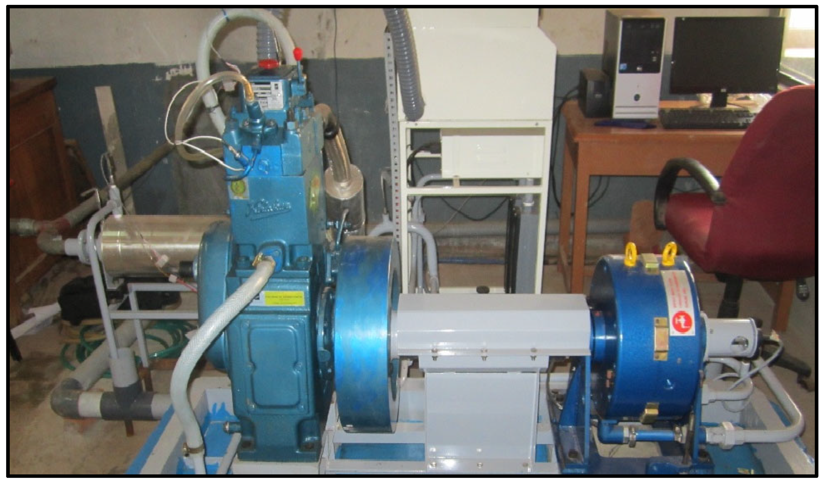
Figure 3 depicts the schematic diagram of the engine setup, while Figure 4 provides a visual representation of the diesel engine test rig setup. Prior to testing the blended fuels, the engine was operated with diesel fuel for approximately 30 min to ensure a stable operating condition. Exhaust emissions from the biodiesel blends were measured at an engine speed of 1500 rpm, a brake power (BP) of 3.7 kW, and a compression ratio (CR) of 17.5:1. The trials were repeated two times, and the middling values of the trial data were considered.

The experiments focused on four biodiesel blends: Jatropha (D60JB30A10, D60JB34A6, D60JB38A2, D60JB40), Honge (D60HB30A10, D60HB34A6, D60HB38A2, D60HB40), Simarouba (D60SB30A10, D60SB34A6, D60SB38A2, D60SB40), and Neem (D60NB30A10, D60NB34A6, D60NB38A2, D60NB40). These blends were tested at different injection operating pressures (200, 205, and 210 bar), a speed of 1500 rpm, and a compression ratio of 17.5:1. Compared to other biodiesel blends, improved performance and emission characteristics were observed for the blends D60JB30A10, D60HB30A10, D60SB30A10, and D60NB30A10, under specific operating conditions: an injection pressure of 205 bar, 80% load, a compression ratio (CR) of 17.5, an injection timing set at 23° prior to top dead center, and a rotational speed of 1500 rpm. Therefore, this article presents the results related to these blends in Section 3.1 and Section 3.2.

3.1. Engine Performance Characteristics

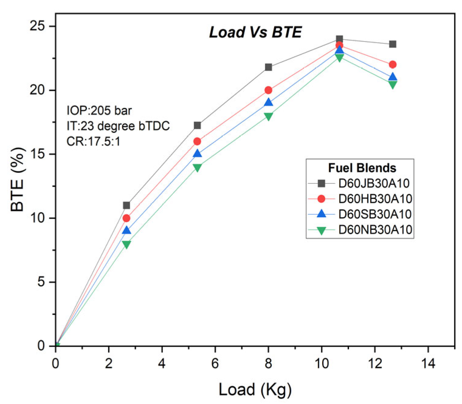
The experiments conducted on Jatropha, Honge, Simarouba, and Neem biodiesel blends yielded interesting results. Among the biodiesel blends, under specific conditions —an injection pressure of 205 bar, 80% load, CR (compression ratio) of 17.5, an injection timing of 23o prior to top dead center, and a rotational speed of 1500 rpm—the highest brake thermal efficiencies (BTE) recorded were 24%, 23.9675%, 23.935%, and 23.9025% for the D60JB30A10, D60HB30A10, D60SB30A10, and D60NB30A10 biodiesel blends, respectively. Notably, the D60JB30A10 blend stood out with the highest brake thermal efficiency of 24% among these blends, as is shown in Figure 5. The exceptional thermal efficiency achieved by the D60JB30A10 Jatropha biodiesel blend can be attributed to its unique chemical properties and their impact on combustion. The introduction of hydrogen peroxide (H₂O₂) into internal combustion engines yields significant impacts on the ignition process. As H₂O₂ decomposes, it releases additional oxygen that fundamentally alters combustion dynamics. This supplementary oxygen facilitates a more complete and efficient combustion of fuel within the engine’s chambers. Biodiesel, including the Jatropha-based blend, contains more oxygen, enhancing fuel oxidation for complete combustion. Its lower carbon-to-hydrogen ratio provides higher energy release per carbon atom, boosting combustion efficiency. Improved ignition characteristics and reduced particulate emissions contribute to smoother and more efficient combustion, minimizing energy losses. Additionally, lower sulfur content and enhanced lubrication properties further optimize efficiency. These chemical traits collectively promote superior combustion efficiency and reduced energy waste, resulting in the blend’s heightened thermal efficiency.

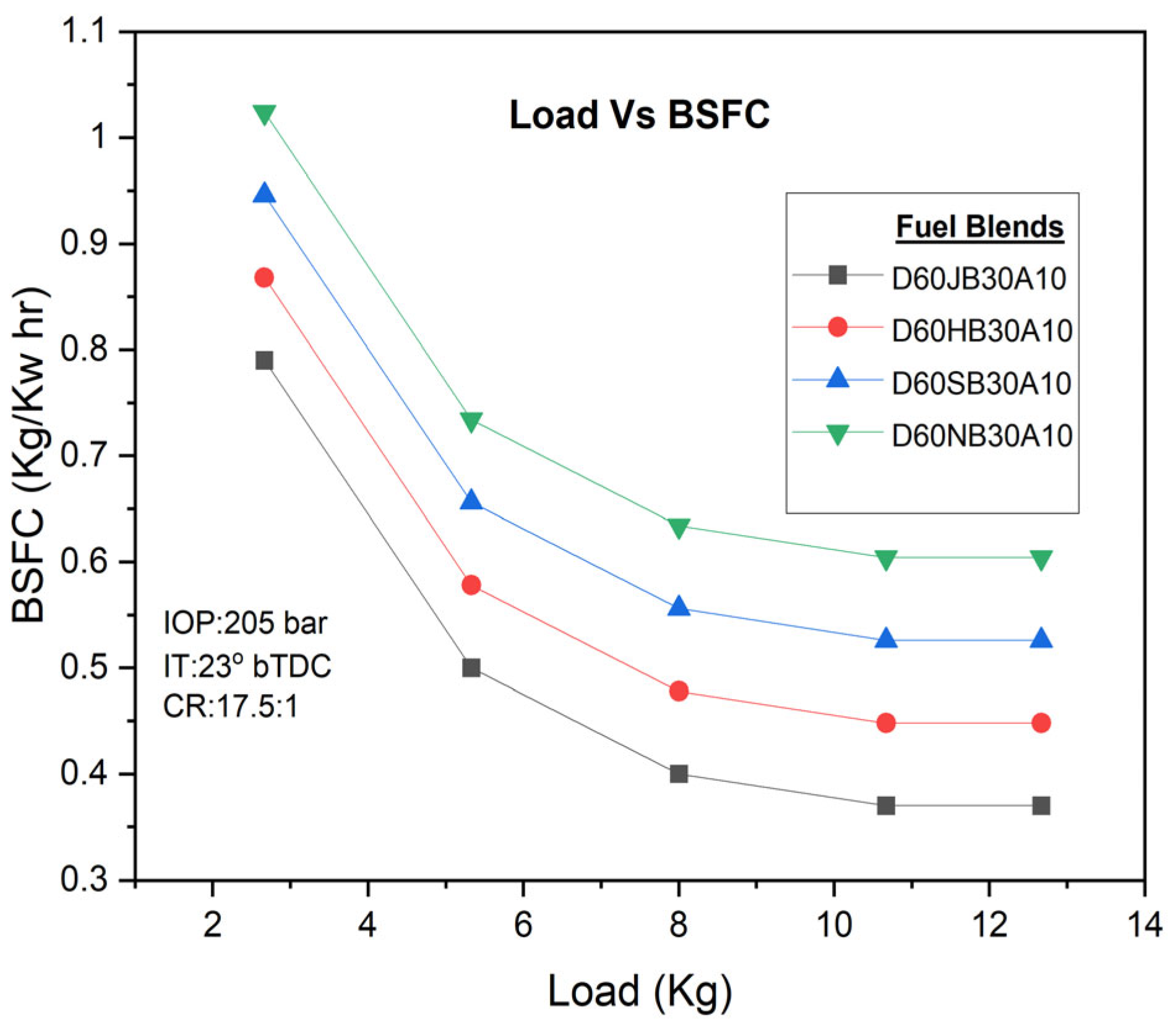
The brake-specific fuel consumption (BSFC) was found to be influenced by the association between spray and ignition characteristics of the fuel. The outcome indicates that the BSFC falls down as the engine load increases, leading to improved fuel consumption rates. However, for the D60JB30A10 fuel blend, the BSFC was found to be higher (i.e., 0.37 kg/kw h) compared to D60HB30A10 (0.448 kg/kw h), D60SB30A10 (0.526 Kg/kw h), and D60NB30A10 (0.604 kg/kw h) biodiesel blends, and the variations are presented in Figure 6. Nevertheless, it was still similar to that of pure diesel.

The combination of H₂O₂ as an oxygenator contributed to the development of a rapid evaporation rate. This, in turn, compacted the combustion advancement time and improved the combustion process, resulting in improved engine presentation.

Overall, the experiments demonstrated that the Jatropha biodiesel blend D60JB30A10, along with an injection operating pressure of 205 bar and a load of 80%, achieved the highest brake thermal efficiency. The addition of H₂O₂ showed the potential in improving combustion and engine performance.

3.2. Engine Emissions Characteristics

The engine’s emissions can be classified into distinct types. NOx emissions primarily stem from the high temperatures in the combustion cavity and blaze, while HC and CO releases result from the improper combustion of fuels and lower combustion temperatures.

The investigation of NOx emissions is conducted under varying engine loads using different fuel blends. Parameters like burning temperature, time period, presence of oxygen, and equivalence proportion significantly influence NOx emissions. The formation of NOx depends on factors such as cylinder temperature, oxygen concentration, and equivalence ratio. The presence of higher oxygen content in the biodiesel blend D60JB30A10 produces high temperature due to complete combustion of fuel, resulting in elevated NOx emissions (720 PPM) as compared to D60HB30A10 (701.5478 PPM), D60SB30A10 (692.2213 PPM), and D60NB30A10 (683.6515 PPM) blends. NOx emissions with engine load for developed biodiesel blends are shown in Figure 7.

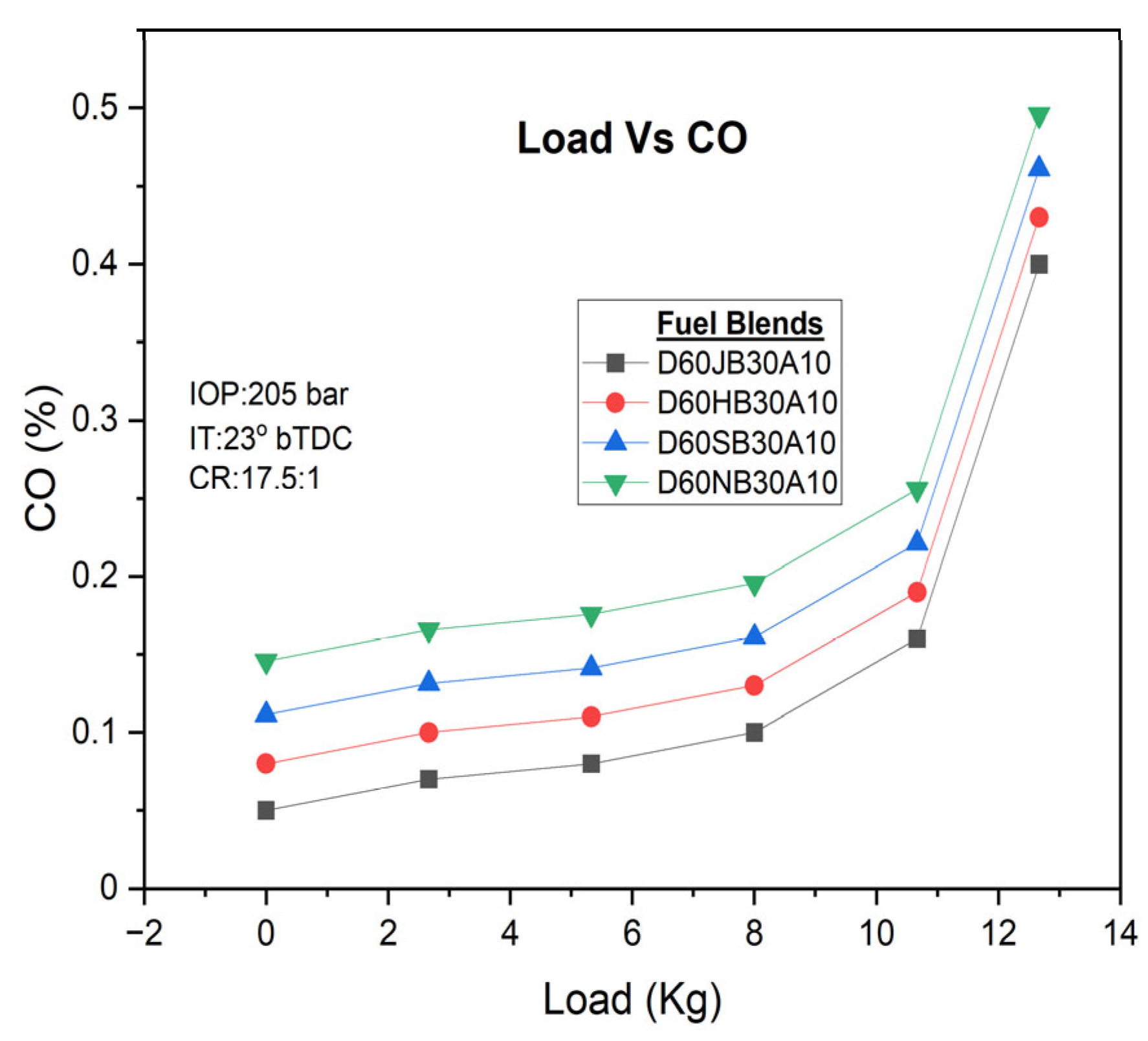
There are different engine loads for various fuel blends. Higher engine loads, especially under full load and partial load conditions, tend to produce higher CO emissions. However, the occurrence of oxygen enrichment in the D60JB30A10 blends result in lower CO emissions (i.e., 0.16 vol%) as compared to D60HB30A10 (0.19 vol%), D60SB30A10 (0.18 vol%), and D60NB30A10 (0.222 vol%) blends. The addition of hydrogen peroxide (H₂O₂) increases the oxygen content, facilitating better carbon oxidation and more complete ignition, thus reducing CO emissions. CO emissions with engine load for developed biodiesel blends are shown in Figure 8.

CO₂ emissions are evaluated under various engine load conditions for different fuel blends, taking into account the presence of hydrogen peroxide. The increased content of H₂O₂ has the potential to influence CO₂ emissions by possibly reducing them. Interestingly, the D60JB30A10 blend demonstrates lower CO₂ emissions (i.e., 7.8 vol%) compared to D60HB30A10 (8.012 vol%), D60SB30A10 (8.2013 vol%), and D60NB30A10 (8.395 vol%) blends. CO₂ emissions with engine load for developed biodiesel blends are shown in Figure 9.

The use of nano-emulsified blended fuel, which undergoes a micro-explosion phenomenon, enhances the atomization (fine droplet size of the emulsion, which increases the surface area for interaction between fuel and air) and combustion of the air–fuel mixture and increases the concentration of OH radicals. As a result, it improves ignition characteristics and contributes to the reduction of CO₂ emissions. This phenomenon is considered to be a significant factor in achieving lower CO₂ emissions during engine operation with nano-emulsified blended fuel.

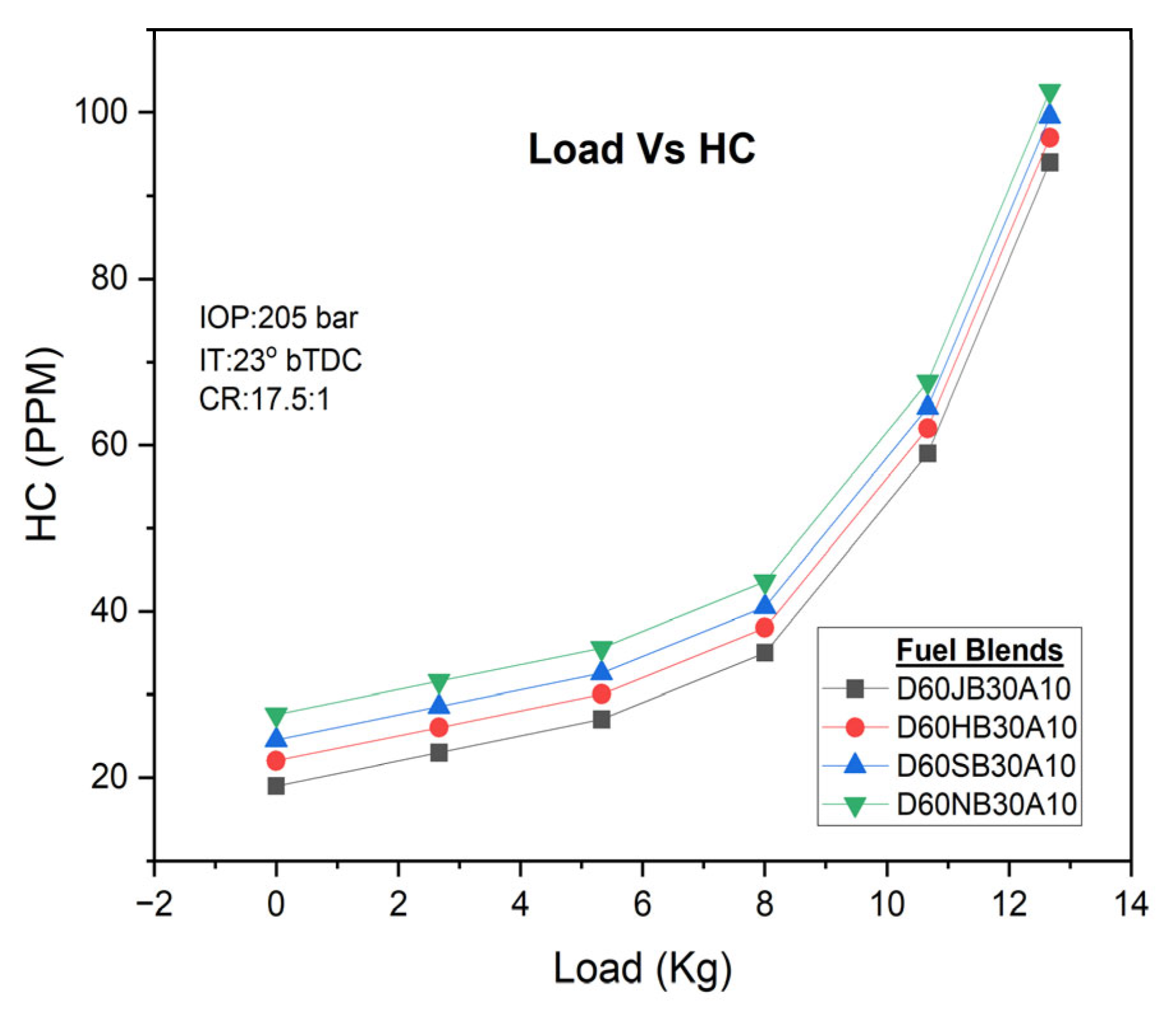
For all fuel blends, higher engine loads result in increased HC emissions. However, the concentration of H₂O₂ plays a significant role in reducing HC emissions. Comparatively, the D60JB30A10 blend exhibits lower HC emissions (i.e., 59 PPM) compared to D60HB30A10 (62.024 PPM), D60SB30A10 (64.0235 PPM), and D60NB30A10 (67.5702 PPM) blends. HC emissions with engine load for developed biodiesel blends are shown in Figure 10. The combination of nano-emulsified fuel blends and the presence of H₂O₂ improves the ignition process and oxidation of unburned or partially burned fuel particles, effectively reducing HC emissions.

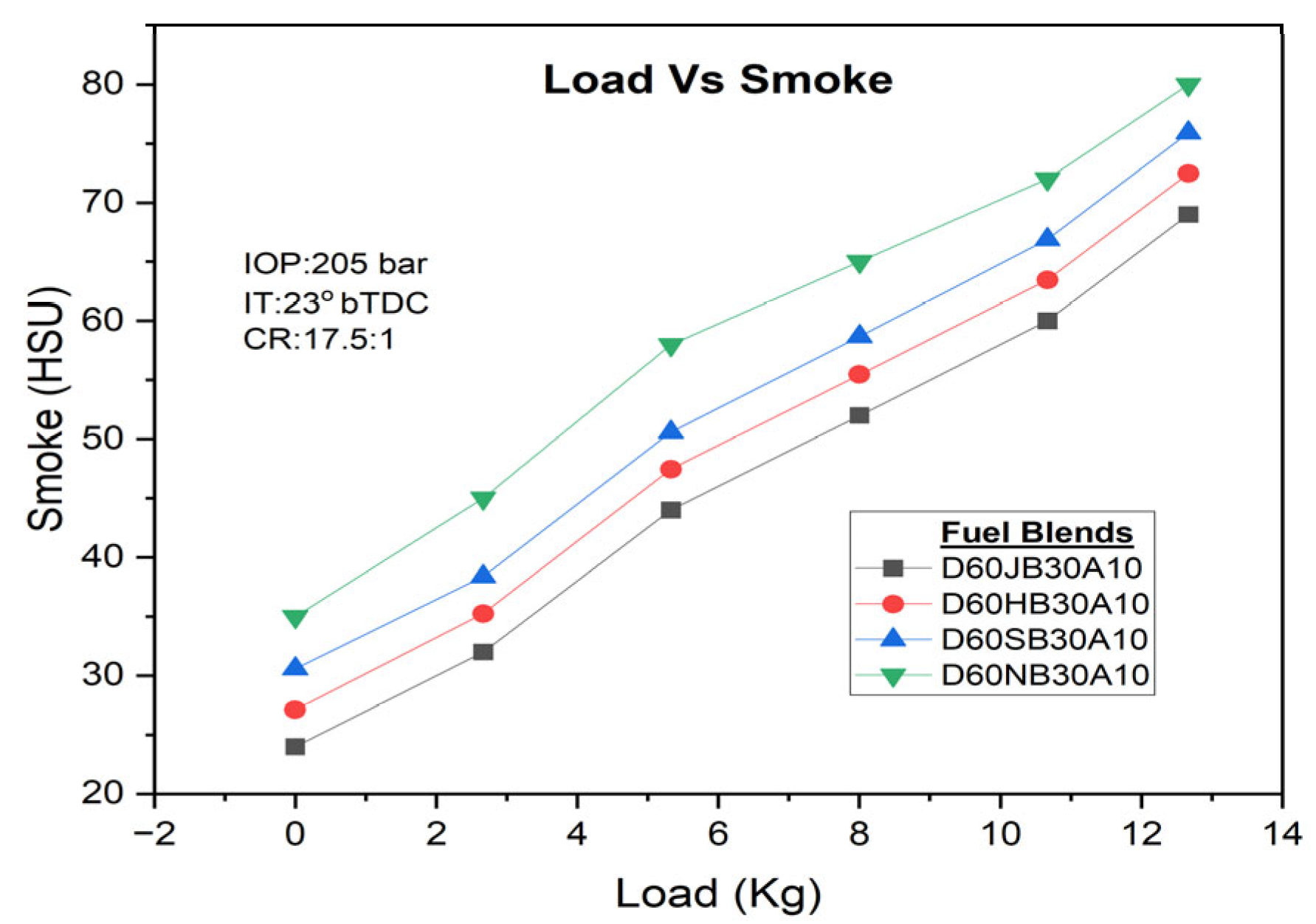
Similarly, smoke emissions also rise with higher engine loads, but the addition of H₂O₂ can substantially decrease smoke emissions. The D60JB30A10 blend demonstrates lower smoke emissions (i.e., 60 HSU) compared to D60HB30A10 (63.452 HSU), D60SB30A10 (66.895 HSU), and D60NB30A10 (70.012 HSU) blends. Smoke emissions with engine load for developed biodiesel blends are shown in Figure 11. The inclusion of H₂O₂ provides additional oxygen, which leads to the more complete breakdown of solid or liquid particles, enhancing the ignition process and contributing to a reduction in smoke emissions.

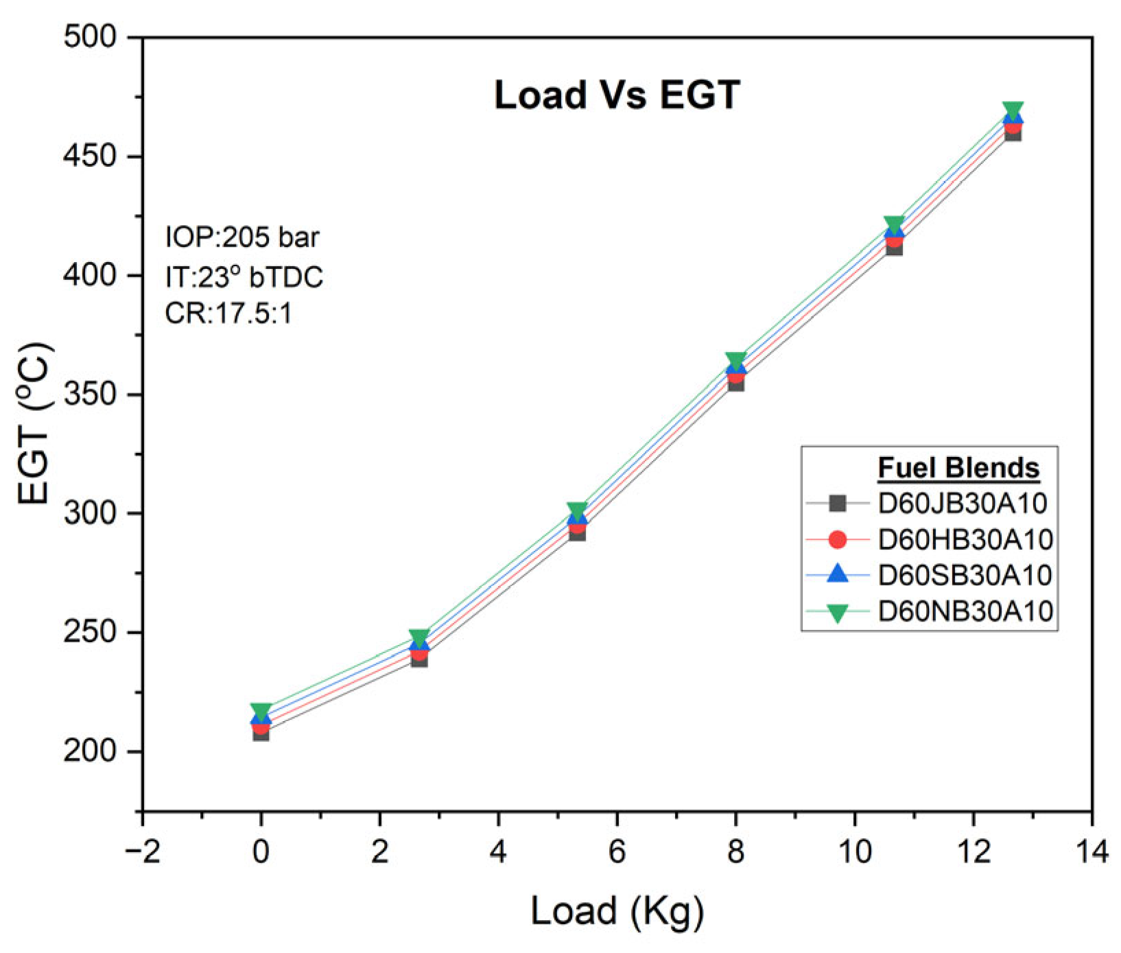
Regarding exhaust gas temperature (EGT), it increases with higher engine loads for all fuel blends. However, increasing the concentration of H₂O₂ leads to a significant rise in EGT. Comparatively, the D60JB30A10 blend exhibits lower EGT (412 °C) compared to D60HB30A10 (415.23 °C), D60SB30A10 (418.568 °C), and D60NB30A10 (422.356 °C HSU) blends, while the lowest EGT is observed for diesel fuel. EGT variation with engine load for developed biodiesel blends is shown in Figure 12.

Overall, the experimental findings indicate that the biodiesel blend D60JB30A10, with its high oxygen content and the influence of hydrogen peroxide, demonstrates favorable emission characteristics. It shows lower levels of NOx, CO, HC, smoke, and EGT compared to other biodiesel blends.

4. Machine Learning: Importing and Analyzing the Data

Data importing involves sourcing and loading the dataset into the Python interpreter. This initial step sets the foundation for all subsequent analysis. Datasets was sourced from Excel formats. The goal is to make the data available for preprocessing and analysis. To analyze the dataset, the first and primary step is to import the necessary Python libraries, such as Pandas, NumPy, Seaborn, Matplotlib, and Warnings. The Warnings library is particularly useful for ignoring any warnings that may arise during execution.

Using the Pandas library, we import the experimental dataset. By observing the shape of the dataset, we can determine that it consists of 361 rows and 13 features.

In order to ensure accurate data for modeling purposes, it is essential to preprocess the entire dataset due to the possibility of errors in manually recorded experimental data. This preprocessing step aims to bring into line the values and make them appropriate for processing by machine learning algorithms.

By importing the required Python libraries and preprocessing the dataset, including cleaning and transforming the data, we establish a foundation for further analysis and modeling tasks.

The following activities were performed:

Preprocessing encompasses tasks like data cleaning, normalization, and feature engineering. Data contain outliers and duplicated values. These issues are addressed through techniques such as imputation and outlier removal. Normalization ensures that features are on similar scales.

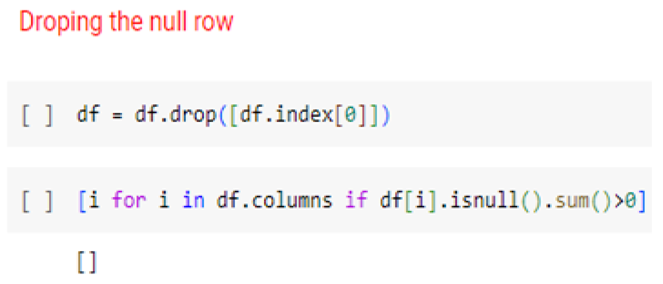
Missing value check: The dataset was examined for any missing values. It was observed that all the features had one common missing value, located at the zeroth index. As a solution, the entire row containing the null value was dropped and a snippet of code has shown in Figure 13. Consequently, the shape of the dataset changed to 360 rows and 13 columns.

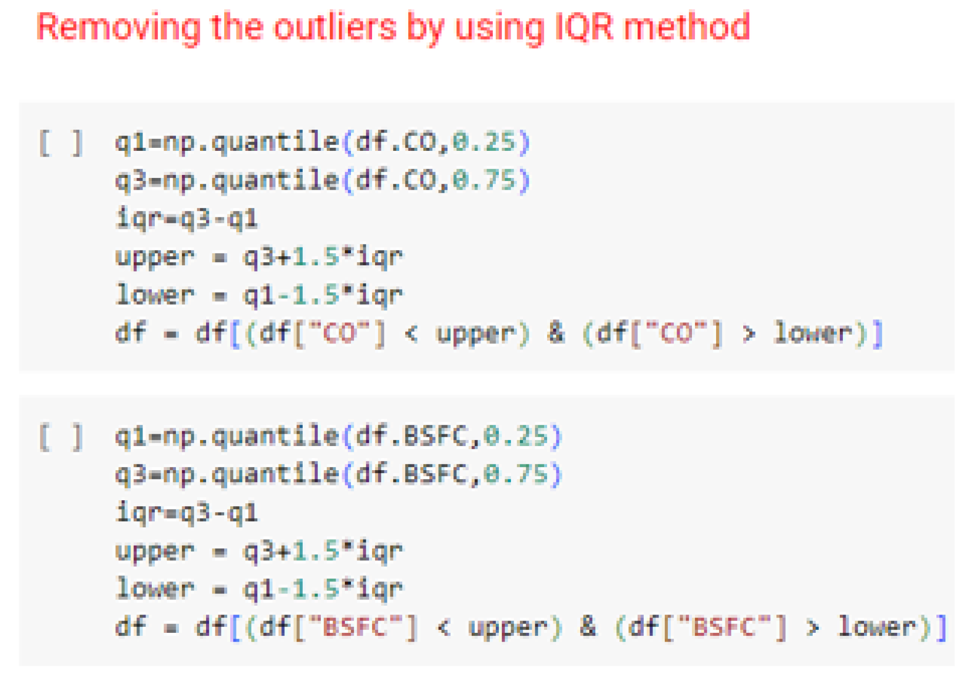
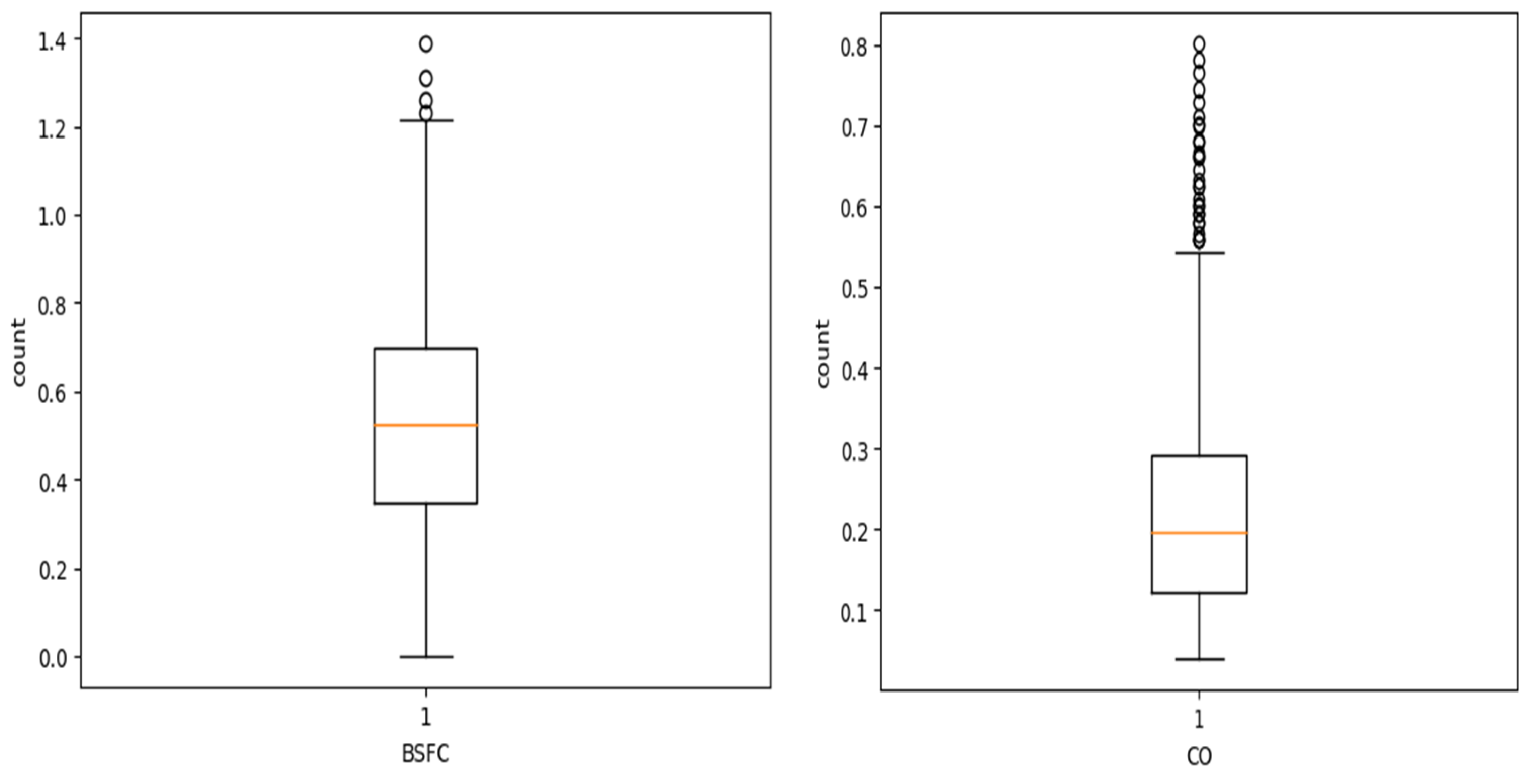
Outlier detection and removal: During univariate analysis, specifically through box plot analysis, it was visually evident that two columns, BSFC and CO, contained outliers, shown in Figure 14. Given that it is a regression problem, it is crucial to eliminate outlier values for accurate prediction of the target column. The outliers were removed using the interquartile range (IQR) method and snippet of code is shown in Figure 15.

The dataset was further processed by addressing missing values and removing outliers to facilitate subsequent analysis and prediction tasks.

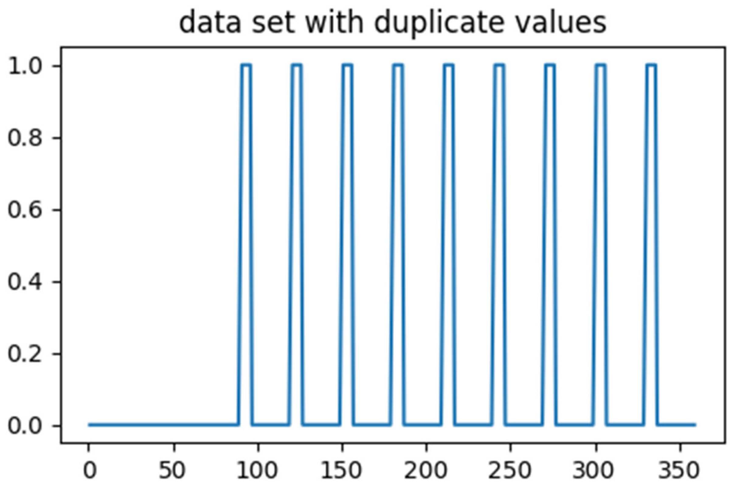
It was observed that there were 54 duplicated rows in the dataset. To ensure accurate analysis of the model, these duplicated rows were dropped. Consequently, the shape of the dataset changed to 276 rows and 12 columns. The visual analysis of the duplicated values is depicted in the Figure 16.

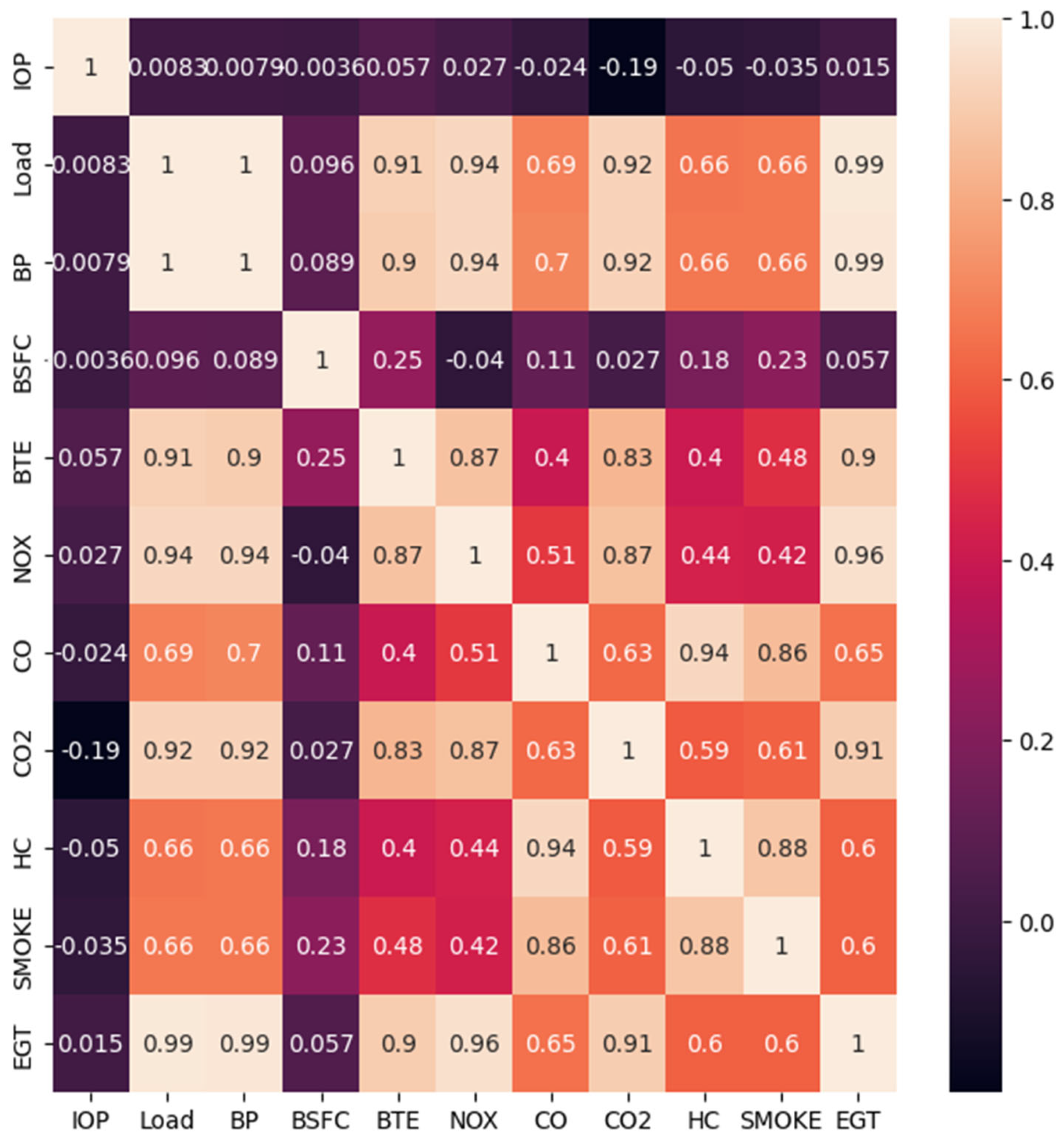
To examine the linearity amongst predictor and response variables, a relationship analysis was performed. Specifically, Pearson’s correlation coefficient was calculated to determine the relationship between input variables and output variables. The correlation coefficient ranges from −1 to +1, with values closer to +1 or −1 indicating a stronger positive or negative correlation, respectively. Figure 3 and Figure 4 depict the correlation between the variables. The analysis revealed that the correlation between the input and output features was moderate, falling within the −1 to +1 range. This suggests the need for appropriate approaches for non-linear models.

Next, the dataset was separated into training and testing sets using an 80:20 ratio. It is advisable to explore different ratios, such as 70:30, 75:25, 85:15, or 90:10, for sensitivity analysis. Randomization was applied during the dataset division to minimize bias and ensure a representative selection of samples and shown in the

Table 3. Sample data set (Top Five rows).

Sl. No.	Fuel	IOP	Load	BP	BSFC	BTE	NOX	CO	CO2	HC	SMOKE	EGT
1	16	200	0	0	0	0	138	0.05	2.7	19	22	210
2	16	200	2.667	0.74	0.84587	10.4	265	0.06	3.32	20	25	270
3	16	200	5.33	1.48	0.48118	16.8	410	0.06	4.92	24	36	320
4	16	200	8.003	2.22	0.36116	21.35	590	0.07	5.8	26	48	375
5	16	200	10.67	2.96	0.33622	24.2	765	0.17	7.6	32	55	455

.

By conducting the correlation analysis and dividing the dataset into training and testing sets, a solid foundation was established for subsequent modeling and evaluation tasks.

The recorded values in the dataset may have different scales, with each feature having a distinct numeric range and are shown in the

Table 4. Descriptive Analysis of the dataset.

Particulars	Count	Mean	Std	Min	25%	50%	75%	Max
	360	180.5	104.06729	1	90.75	180.5	270.25	360
IOP	360	205	4.088165	200	200	205	210	210
Load (kg)	360	6.526167	4.417539	0	2.667	6.6715	10.67	12.67
B.P. (kW)	360	1.841778	1.270335	0	0.74	1.85	2.96	3.7
BSFC (kg/kW.hr)	360	0.51732	0.321067	0	0.347866	0.524112	0.699893	1.38844
BTE (%)	360	14.597611	7.97892	0	9.599375	17.17625	20.84313	25.57
NOX (PPM)	360	406.20042	264.06918	36.847	156.5076	357.1852	601.8145	980
CO (%Vol)	360	0.23776	0.167199	0.04	0.1209	0.19572	0.29181	0.80181
CO2 (%Vol)	360	5.351196	1.9092	2.5	3.5219	5.4181	7.4	8.5442
HC (PPM)	360	56.072071	28.447001	17	33.3098	51.0246	75.02415	128.577
SMOKE (HSU)	360	61.595031	20.751297	20	48	62	75.931	111.365
EGT (0C)	360	333.6266	91.204363	196	249.5818	320	419.928	480.233

. These variations in scales can create challenges in interpreting the results of the modeling problem. Machine learning algorithms generally work with numeric values, and treating each data point quantitatively can significantly impact the modeling process. Moreover, when the ranges of different features vary widely, it can lead to substantial effects on the model outcomes. To mitigate such anomalies, it is crucial to normalize the data to a standardized range of −1 to +1. This can be achieved using a standard scalar normalization. By normalizing the training dataset, the potential impact of varying numeric ranges is minimized, enabling more effective modeling and analysis.

Feature Selection: in the case of a regression problem, particularly when conducting linear regression, it is essential to adhere to certain assumptions. One crucial assumption is checking for multicollinearity between the independent variables and the target variable. To assess multicollinearity, the variance inflation factor (VIF) method was utilized. It was observed that some columns had VIF values greater than 10, indicating the presence of multicollinearity. As a result, those columns were dropped from the dataset, resulting in a new shape of 360 rows and 9 columns.

Another significant assumption to consider is autocorrelation in the regression model. Autocorrelation can be examined using tests such as the Durbin–Watson test. In this dataset, no signs of autocorrelation were detected, as indicated by the test values.

By addressing the assumptions related to multicollinearity and autocorrelation, the dataset was further prepared for the linear regression analysis and detailed methodology has been shown in the Figure 17.

Based on the Figure 18 and

Table 5. Correlation between the features.

Particulars	IOP	Load	BP	BSFC	BTE	NOX	CO	CO2	HC	SMOKE	EGT
IOP	1	0.00832	0.00794	−0.00358	0.05748	0.026539	−0.02425	−0.19009	−0.0497	−0.03481	0.01524
Load	0.00832	1	0.99906	0.095805	0.91415	0.935711	0.687026	0.922566	0.65528	0.663807	0.98627
BP	0.007938	0.99906	1	0.089115	0.902	0.939528	0.701784	0.921648	0.66325	0.664946	0.98602
BSFC	−0.00358	0.09581	0.08912	1	0.25429	−0.03994	0.114615	0.027125	0.17709	0.230984	0.05747
BTE	0.057479	0.91415	0.902	0.254287	1	0.873651	0.400161	0.832741	0.40407	0.477505	0.90225
NOX	0.026539	0.93571	0.93953	−0.03994	0.87365	1	0.505764	0.869285	0.43729	0.424098	0.96303
CO	−0.02425	0.68703	0.70178	0.114615	0.40016	0.505764	1	0.626806	0.93831	0.855134	0.64601
CO2	−0.19009	0.92257	0.92165	0.027125	0.83274	0.869285	0.626806	1	0.58638	0.607006	0.90695
HC	−0.0497	0.65528	0.66325	0.177092	0.40407	0.437289	0.93831	0.586379	1	0.880364	0.60037
SMOKE	−0.03481	0.66381	0.66495	0.230984	0.47751	0.424098	0.855134	0.607006	0.88036	1	0.60155
EGT	0.01524	0.98627	0.98602	0.05747	0.90225	0.963029	0.646012	0.906954	0.60037	0.601545	1

, it can be observed that the correlation analysis reveals the following findings:

The features Load, BP, NOx, CO₂, and EGT exhibit a strong positive correlation with the target column. This implies that any small changes in these features will have a direct impact on the target column.

The features CO, HC, and Smoke also show a positive correlation with the target column, but the correlation is not as strong as with the previously mentioned features. Consequently, variations in these independent columns may not result in significant variations in the target column.

Overall, the analysis suggests that the Load, BP, NOx, CO₂, and EGT features are highly influential in predicting the target column, while the CO, HC, and Smoke features have a relatively lesser impact. This understanding of the correlation between the features and the target variable is crucial for further modeling and analysis.

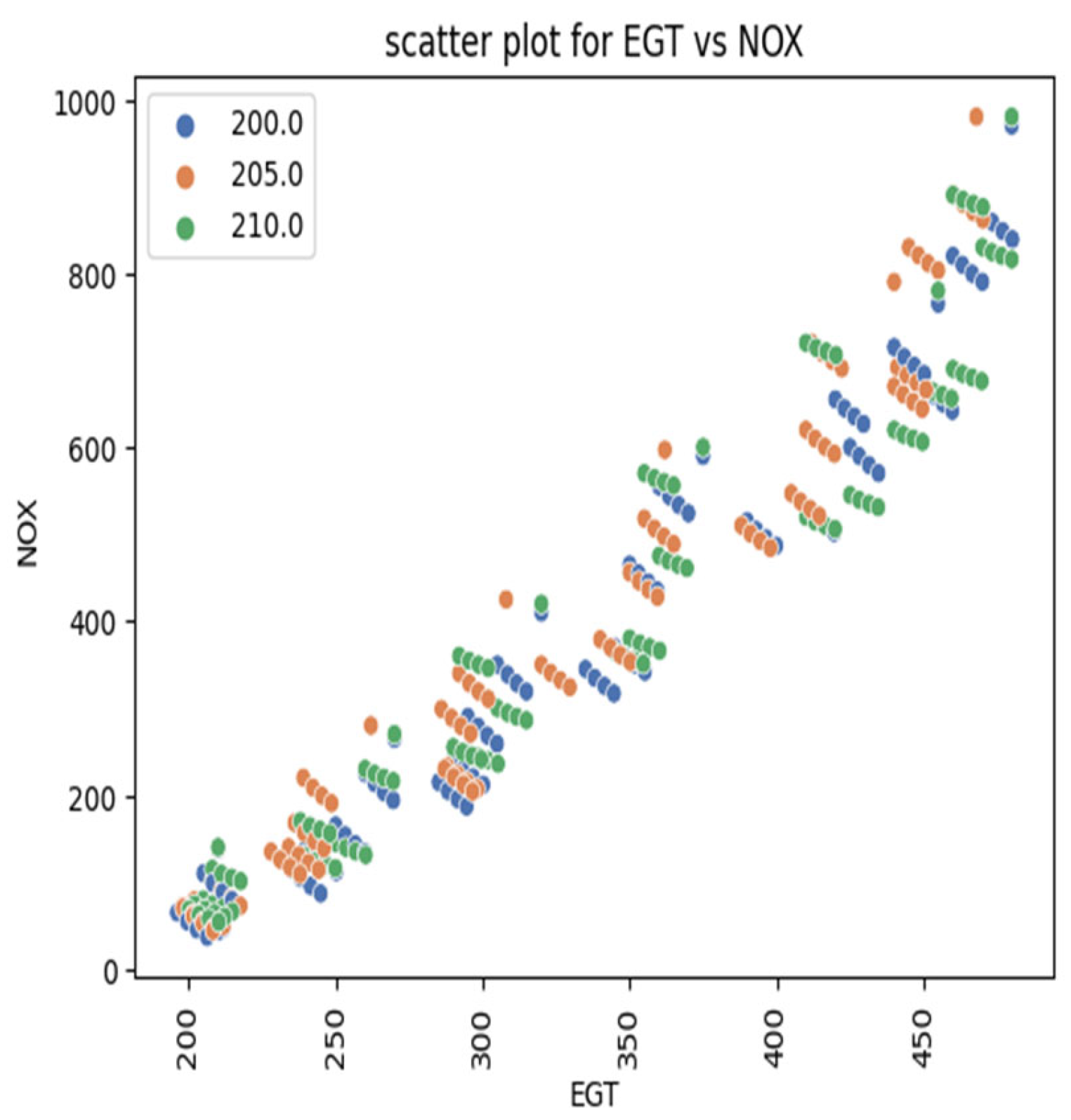
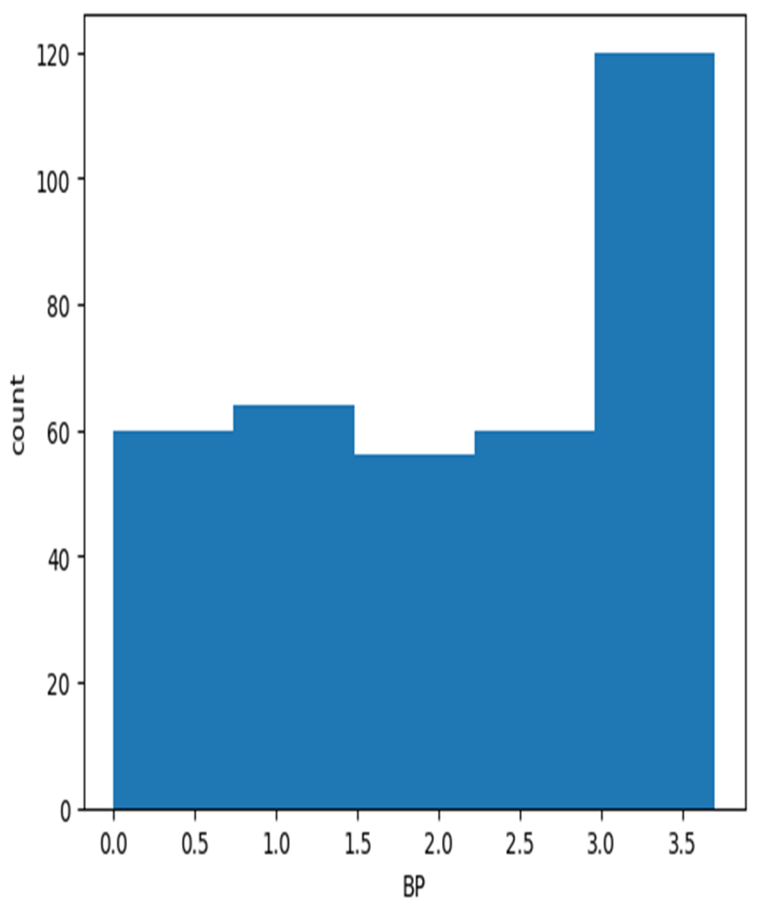
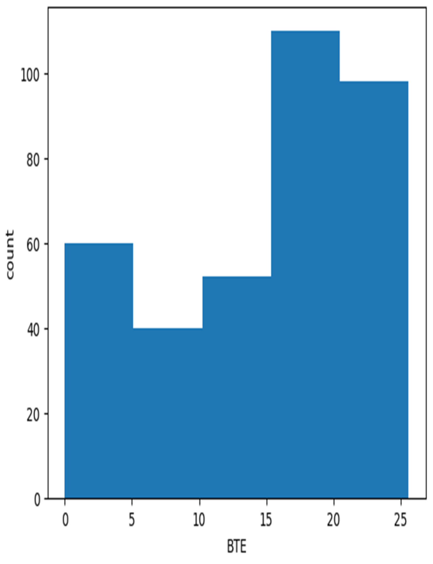
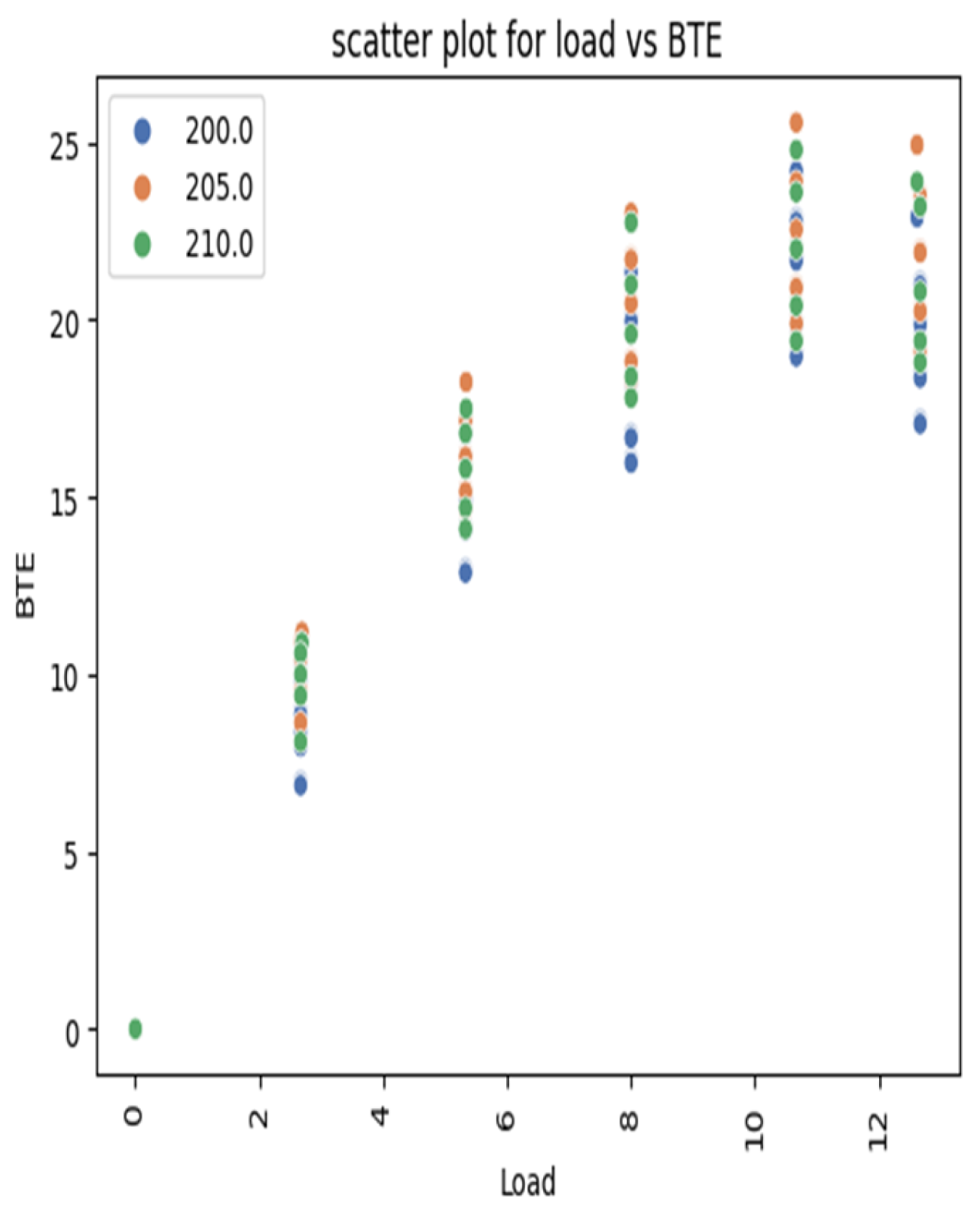
EDA (Exploratory data analysis) involves analyzing the dataset to understand its structure and relationships. Statistical summaries, data visualizations, and correlation analyses are employed. EDA helps identify patterns, trends, and potential insights, aiding in feature selection and guiding model choice; scatter plot for BTE and NO_x are shown in the Figure 19 and Figure 20, and histograms are shown in the Figure 21 and Figure 22 of EDA are shown below.

4.1. Prediction Modeling

Once the data is prepared, model building begins. Different algorithms, such as decision trees, random forest regressor, Linear regression and XG Boost regressor are selected based on the problem’s nature. The dataset is split into training and testing sets to facilitate model training and validation.

All available regression models are being considered for model development in this regression problem, with the aim of selecting the most suitable one.

4.1.1. Linear Regression

Linear regression is a tranquil and straightforward statistical approach employed for predictive analysis to demonstrate the association between continuous variables. It illustrates the linear connection between the independent variable (X-axis) and the dependent variable (Y-axis), hence referred to as linear regression. When a single input variable (x) is involved, it is known as simple linear regression, while multiple linear regression refers to cases where more than one input variable is considered. The model yields a straight line with a slope that describes the relationship between the variables.

Figure 23 represents a linear correlation between the dependent variable and independent variables. As the independent variable (x) increases, the dependent variable (y) also increases. The blue line on the graph represents the best-fit straight line, which is derived from the available data points. The goal is to find a line that optimally represents the data.

Linear regression utilizes the traditional slope-intercept form to determine the best-fit line, which can be expressed as follows:

$$y=mx+c\to y=a_0+a_{1}x$$

where, y = Dependent Variable, x = Independent Variable, a₀ = intercept of the line, a₁ = Linear regression coefficient or slope.

In this equation, y represents the dependent variable, x represents the independent variable, m represents the slope of the line, and c represents the y-intercept.

Upon analyzing this prediction, we note that the intercept and coefficient values are 13.94, −0.1325696, 0.84535725, 1.88961188, 5.2897039, −3.22701143, 2.98569011, and 2.45294863. The best-fit line, accompanied by the cost function illustrated earlier, reveals the corresponding residual values presented in the

Table 6. Comparison of actual and predicted values using the Linear regression algorithm.

	Actual	Prediction	Residuals
108	19.9675	22.599717	2.632217
19	0	1.793336	1.793336
229	0	1.251205	1.251205
67	0	2.372716	2.372716
322	18.8225	18.730705	0.091795

. Notably, the algorithm shows no signs of under fitting or over fitting, indicating that it is a well-generalized model with both low bias and low variance. Impressively, the scores achieved for the training and test datasets stand at 92.53% and 100%, respectively.

4.1.2. Decision Tree Regressor

The Decision Tree stands as one of the most widely used and practical approaches for supervised learning. It possesses the ability to tackle both Regression and Classification tasks, although its practical application leans more towards Classification. This tree-structured classifier is comprised of three types of nodes. The journey begins at the Root Node, representing the entire sample, and may branch out into further nodes. The Interior Nodes capture the dataset’s features, while the branches embody the decision rules. Ultimately, the outcome is represented by the Leaf Nodes.

The algorithm proves highly beneficial for solving decision-related problems. When applied to a specific data point, it follows a series of True/False questions, traversing the entire tree until it reaches the relevant leaf node. The final prediction is obtained by averaging the dependent variable’s value at that particular leaf node. Through multiple iterations, the Decision Tree adeptly predicts precise values for data points.

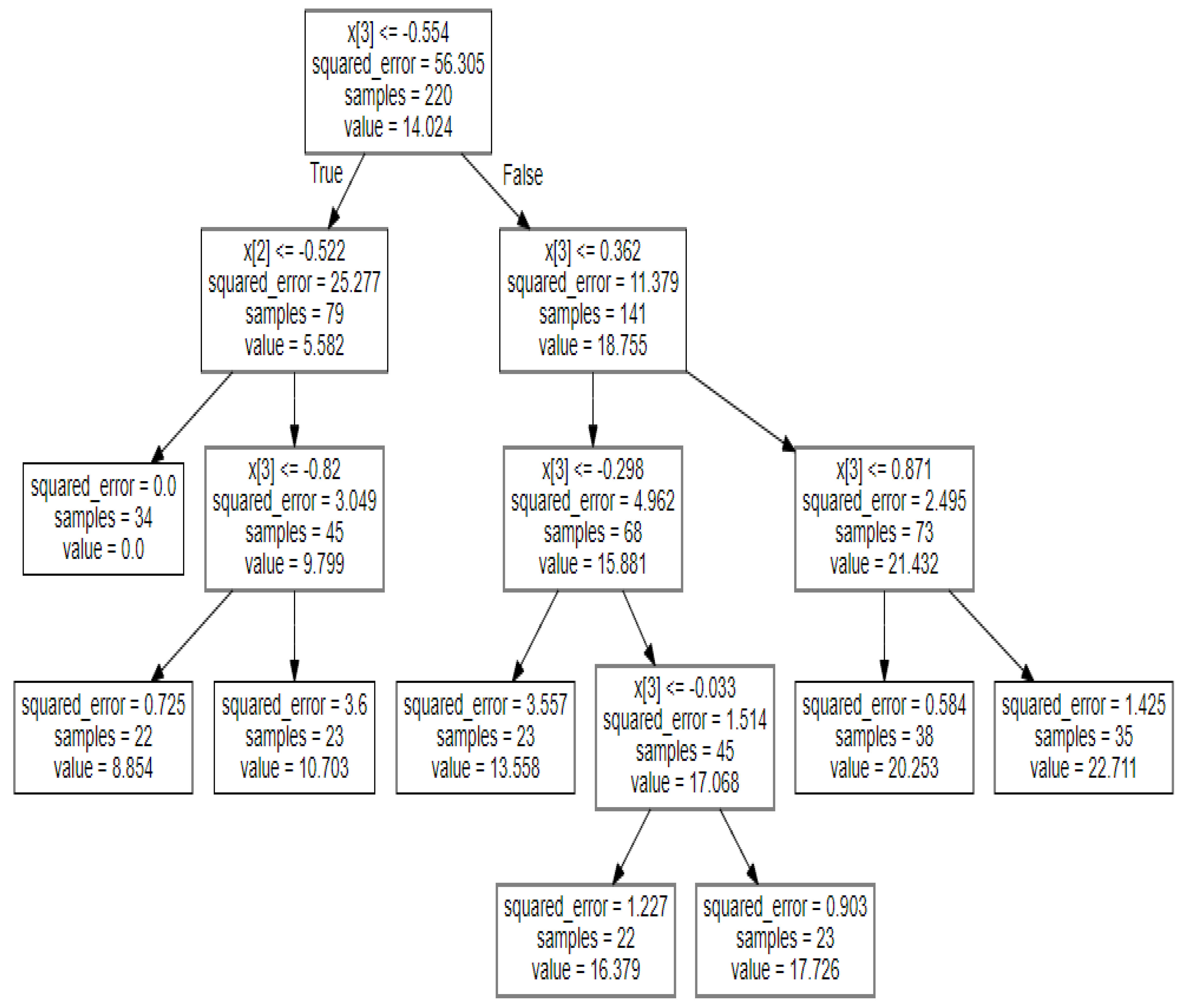
From the decision tree regressor, it is evident that the residuals have decreased in comparison to linear regression. The error function also experiences some reduction, leading to an improvement in the model’s score. As a result, a more generalized model is achieved. Figure 24 illustrates the development and division of the tree based on the squared function, and the leaf nodes make predictions for the target values, as displayed in the

Table 7. Comparison of actual and prediction values using the Decision Tree Regressor algorithm.

	Actual	Prediction	Residuals
108	19.968	21.8	1.8325
19	0	0	0
229	0	0	0
67	0	0	0
322	18.823	17.8025	1.02

. The scores for the decision tree regression have notably increased when compared to linear regression, reaching 97.57% for the training dataset and a perfect 100% for the test dataset.

4.1.3. Random Forest Regressor

RF is an ensemble learning technique based on bagging, commonly used for both classification and regression tasks. It utilizes a framework of decision trees to make predictions. The process involves providing bootstrap samples (randomly selected subsets with replacement) to multiple decision trees, with each tree producing its own output. The final prediction is then determined by averaging the results from all the decision trees.

The Random Forest Regression follows the following steps:

Randomly select M data points from the original dataset.

Determine the number of decision trees (N) to build.

Build decision trees based on subsets of the data points.

Repeat steps 1 and 3 to create multiple decision trees.

The final predicted output (Y) is obtained by averaging the outputs (y1, y2, y3, …, yN) of all the decision trees.

In the Random Forest algorithm, the dataset is divided into five equal subsets, where some rows may be repeated across subsets, and each subset is given equal weight. Predictions are made based on the mean evaluation.

When comparing the performance scores, the Random Forest Regressor outperforms the Decision Tree Regressor. It achieves an impressive 99.34% accuracy on the training dataset and a perfect 100% accuracy on the test dataset.

4.1.4. XG Boost

XG Boost (Extreme Gradient Boosting) is a powerful library for prediction and classification tasks. Its key advantages are speed, scalability, and parallel computation, outperforming other algorithms. It converts weak learners into strong ones using boosting and employs a second-order Taylor expansion to mitigate overfitting, resulting in a highly effective model [4]

$${\widehat{y}}_i=\mathsf{\theta }\left(x_i\right){{\displaystyle \sum }}_{k=1}^N{f}_k\left(x_i\right),f_k\mathsf{\varepsilon }\mathrm{F}$$

$$F=\left\{f|f\left(x\right)=w_q\left(x\right)\right\}$$

In the provided equation:

K denotes the number of regression trees.

F represents regression trees sets.

$\widehat{y}$ signifies the weight vector of regression tree.

(x) indicates the kth decision tree’s input value.

y_i represents the value of prediction.

x_i is the value of input.

f_k refers to the kth decision tree.

w represents regression tree’s weight.

q represents the structure of the tree.

As follows, the purpose function can be stated as

$$0=l\left(y_i, \widehat{y}\right)+{{\displaystyle \sum }}_{k=1}^k\mathsf{\Omega }f\left(k\right)$$

In the provided context:

The expression (y_i, $\widehat{y}$) denotes the discrepancy of the real and predicted values.

$\mathsf{\Omega }$ represents the regularization rate, which is employed to prevent overfitting of the representation.

To achieve optimized results, certain iterations are executed.

The above equations can be derived through a specific deduction process.

$$0^{\left(t\right)}={\displaystyle \sum }_{i=1}^{N}l\left(y_i, {\widehat{y}}^{\left(t-1\right)}+g_i{f}_t\left(x_i\right)+\frac{1}{2}{h}_i{f}_t{}^2\left(x_i\right)\right)+\mathsf{\Omega } \left(f_t\right)$$

$$g_i=\partial { }_{\widehat{y}\left(t-1\right)}l\left(y_i, {\widehat{y}}^{\left(t-1\right)}\right)$$

$$h_i={\partial }^2{}_{\widehat{y}\left(t-1\right)}l\left(y_i, {\widehat{y}}^{\left(t-1\right)}\right)$$

where (t) is the projected rate of the ith trial in the tth trial and N is the entire i quantity of decision tree.

In the XG Boost algorithm, the dataset is sequentially passed through various models with varying weights. The errors from previous models are then propagated to the next models, and through this iterative process, the errors in the dataset are gradually reduced and comparisons of actual and predicted values are shown in

Table 8. Comparison of actual and prediction values using the XG Boost algorithm.

	Actual	Prediction	Residuals
108	19.9675	21.227884	1.260384
19	0	−0.009527	0.009527
229	0	−0.050274	0.050274
67	0	0.004921	0.004921
322	18.8225	17.989958	0.832542

. Eventually, after passing through all the models, the errors are minimized to their least values.

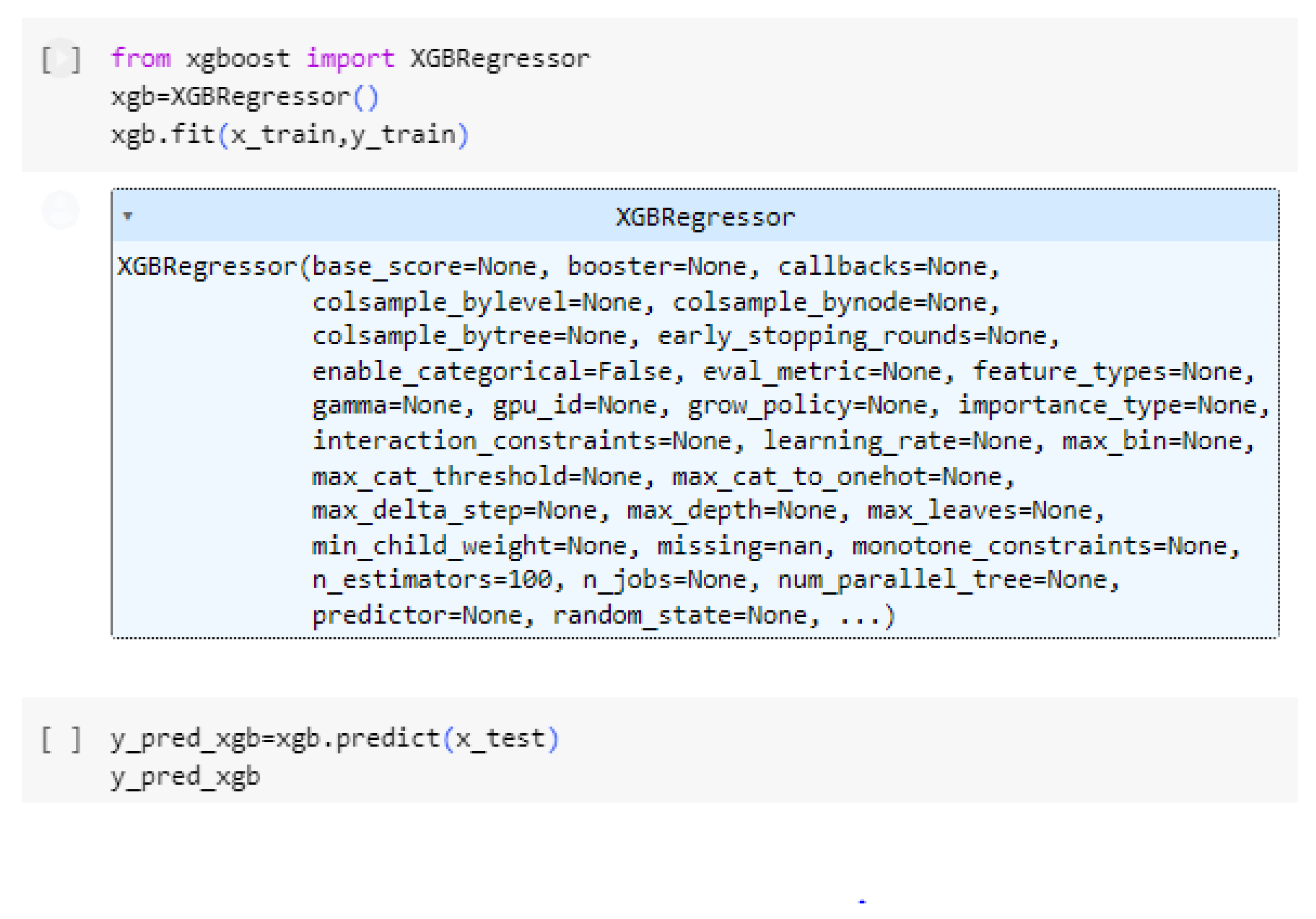
This reduction in errors is evident from the high scores achieved on both the exercise and trying datasets, with scores of 99.99% and 100%, respectively. These high scores indicate that the XG Boost model is a generalized one with low bias and low variance. In other words, it performs well on both the training and testing data, demonstrating its ability to make accurate predictions on unseen data as well. A snippet of XG boost code has shown in the Figure 25.

5. Model Hyperparameter Tuning

Hyperparameters are settings that influence a model’s behavior and performance. Tuning involves adjusting these parameters to optimize model performance.

In the proposed study, the process of hyperparameter tuning using Grid Search is conducted to carefully select the hyperparameters for every regression model, specifically the Decision Tree Regressor, Random Forest Regressor, and XG Boost. The primary objective is to identify the ideal combination of hyperparameters that maximizes prediction accuracy.

Grid Search involves creating and evaluating multiple models with different combinations of hyperparameters. For the Decision Tree Regressor, the hyperparameters being tuned include Max Depth, Min Samples Split, Min Samples Leaf, and Max Features. Similarly, for the Random Forest Regressor, the hyperparameters being optimized are Number of Trees, Max Depth, Min Samples Split, and Max Features. As for XG Boost, the hyperparameters being tuned are Number of Trees, Learning Rate, Max Depth, and Subsample.

By systematically evaluating various combinations of these hyperparameters, Grid Search helps identify the optimal set of hyperparameters that result in improved prediction accuracy for each regression model. This approach overcomes the limitations of trying all possible combinations and saves time compared to an exhaustive search. The selected hyperparameters listed in

Table 9. ML algorithms and its hyperparameters.

Algorithms	Learning Type	Hyperparameter
Decision tree regressor	Tree based	Max depth: 1, 3, 5, 7, 9, 11, 12 Min samples leaf: 1, 2, 3, 4, 5, 6, 7, 8, 9, 10 Min weight fraction leaf: 0.1, 0.2, 0.3, 0.4, 0.5, 0.6, 0.7, 0.8, 0.9 Max features: auto, “log2”, “sqrt”, None Max leaf nodes: None, 10, 20, 30, 40, 50, 60, 70, 80, 90
Random Forest Regressor	Bagging	Bootstrap: TRUE max depth: 80, 90, 100, 110 max features: 2, 3 min samples leaf: 3, 4, 5 min samples split: 8, 10, 12 n estimators: 100, 200, 300, 1000
XG Boost	Boosting	Learning rate: 0.05, 0.10, 0.15 max depth: 3, 4, 5, 6, 8 min child weight: 1 3, 5, 7 gamma: 0.0, 0.1, 0.2 Col sample by tree: 0.3, 0.4

represent the best choices obtained through the Grid Search optimization process.

6. Model Evaluation

In regression problems, the goal is to establish a mapping between the actual values of the dependent variable and the predicted values obtained from the models. Evaluating the performance of individual regression models can be done using various performance metrics, such as R2-Score, RMSE (Root Mean Squared Error), MSE (Mean Squared Error), and MAE (Mean Absolute Error).

R Squared (R2)

The R2-score assesses the model’s performance but does not directly indicate its error. It is a widely used goodness-of-fit indicator for regression models and takes values between 0 and 1. A value of 0 implies that the model does not explain any variability in the response data around the mean. On the other hand, a value of 1 suggests that the model perfectly fits the data without any faults.

The R Squared equation is as follows.

$$R^2=1-\frac{{{\displaystyle \sum }}_{k=1}^N(y_k-{\widehat{y}}_k)}{{{\displaystyle \sum }}_{k=1}^N(y_k-{\overline{y}}_k)}$$

In the provided context:

N denotes the data points.

y_k represents the real yield.

${\widehat{y}}_k$ represents the yield of prediction.

${\overline{y}}_k$ is the mean value.

Root Mean Squared Error (RMSE)

The root mean squared error (RMSE) is a commonly used metric for evaluating the performance of regression models. It is calculated by taking the square root of the mean of the squared differences between the actual values and the predicted values. RMSE’s straightforward interpretation of loss is due to its output being in the identical unit like preferred output parameter.

$$RMSE=\sqrt{\frac{1}{N}{\displaystyle \sum }_{k=1}^N(y_k-{\widehat{y}}_k)}$$

In the given context

N represents the total number of data points.

Y_k represents the expected value.

${\widehat{y}}_{k }$ represents the predicted value.

Mean Squared Error (MSE)

MSE (Mean Squared Error) is one of the most extensively used and straightforward metrics, diligently connected to Mean Absolute Error (MAE) with a minor difference. It comprises of finding the squared change among the actual and predicted values in a regression model. The MSE represents the average squared distance between the actual and predicted values. By squaring the differences, we stop the termination of negative terms, which is one of the benefits of using MSE as a metric for evaluating the performance of a regression model.

$$\mathrm{MSE}=\frac{1}{\mathrm{n}}\sum {\left(\mathrm{y}-\widehat{\mathrm{y}}.\right)}^2$$

where ${\left(\mathrm{y}-\widehat{\mathrm{y}}.\right)}^2$= the square of the difference between actual and predicted

Mean Absolute Error (MAE)

The MAE (Mean Absolute Error) score is obtained by taking the average of the absolute error values, where the absolute function ensures that the values are turned positive. This means that the difference between an expected value and a predicted value can be either positive or negative, but when calculating the MAE, the value will always be positive when measured

The MAE is intended as follows:

$$MAE=\frac{1}{\mathrm{n}}{\displaystyle \sum }_{i=1}^N(y_i-{\widehat{y}}_i)$$

where ‘n’ is the whole volume of data points, y_i is the projected value and ${\widehat{y}}_i$ is the anticipated rate.

7. Comparison of Algorithms

Evaluation metrics such as R2-Score, RMSE, MSE, and MAE are essential for assessing the performance of learning models. The evaluation metric values for the performance and emission characteristics of an engine are presented in

Table 10. Comparison of Algorithms on Evaluation Matrices.

Learning Algorithms	MAE	MSE	RMSE	R2-Score
				Trained Value	Test Value
Linear Regression	1.719	4.587	1.311	0.925	1
Decision tree regressor	0.496	0.727	0.704	1	1
Tuned Decision tree regressor	0.7858	1.489	1.220	0.9757	1
Random forest regressor	0.425	0.441	0.664	0.998	1
Tuned Random Forest regressor	0.659	.07259	0.8520	0.9934	1
XG Boost	0.292	0.248	0.540	0.999	1
Tuned XG Boost	0.6059	0.5929	0.7784	0.9976	1

. By comparing Linear Regression, Decision Tree Regressor, Random Forest Algorithm, and XG Boost learning algorithms using these metrics, we can gain insights into their performance.

A higher R2-Score value, approaching 1, signifies a strong fit of the model with the given dataset. From Table 10, it can be observed that the R2-Score values for the algorithms, except for XG Boost, are very close to 1, indicating a favorable fit with the data.

Regarding the error metrics (MAE, MAPE, and RMSE), the values are found to be close to 0 for Linear Regression, Decision Tree Regressor, Random Forest Regressor, and XG Boost Regressor. The low error values suggest that the ensemble learning algorithms are well-suited for making accurate predictions regarding the performance of a single-cylinder four-stroke diesel engine.

In conclusion, based on the evaluation metrics, the ensemble learning algorithms show promising results and are recommended for predicting the performance of the single-cylinder four-stroke diesel engine.

After evaluating all the models, it has been determined that XG Boost, without hyperparameter tuning, demonstrates the lowest RMSE (Root Mean Squared Error) value. Based on this evaluation, XG Boost can be regarded as the best model for predicting the BTE (Brake Thermal Efficiency) values using the given dataset in

Table 11. Comparison of output values for all the models.

Sl. No	Predicted Values for Linear Regression	Predicted Values for Decision Tree Regressor	Predicted Values for Decision Tree Regressor with Hyperparameter Tune	Predicted Values for Random Forest Regression	Predicted values for Random Forest Regressor with Hyperparameter Tune	Predicted Values for XG Boost Regressor	Predicted Values for XG Boost Regressor with Hyperparameter Tune
0	22.599717	21.8	22.711143	21.312825	21.158976	21.227884	20.5627
1	1.793336	0	0	0	0.084671	−0.009527	−0.4792
2	1.251205	0	0	0	0.760643	−0.050274	1.37636
3	2.372716	0	0	0.095	1.926485	0.004921	−0.191
4	18.730705	17.8025	17.725978	17.858625	17.733506	17.989958	18.1769

.

8. Conclusions

Tests were directed on a single-cylinder four-stroke diesel-powered engine, using various blends of Jatropha biodiesel (D60JB30A10, D60JB34A6, D60JB38A2, D60JB40), Honge biodiesel (D60HB30A10, D60HB34A6, D60HB38A2, D60HB40), Simarouba biodiesel (D60SB30A10, D60SB34A6, D60SB38A2, D60SB40), and Neem biodiesel (D60NB30A10, D60NB34A6, D60NB38A2, D60NB40), under different injection operating pressures (200, 205, and 210 bar), 1500 rpm speed, and 17.5:1 compression ratio (CR).

The results indicated that the Brake Thermal Efficiency (BTE) of the engine improved due to the inclusion of H₂O₂ (hydrogen peroxide) in both diesel and biodiesel fuels. Among the blends, D60JB30A10 achieved the highest BTE at 80% load and 205 bar IOP.

Furthermore, the mixing of H₂O₂ as a fuel oxidizer led to a reduction in CO emissions and improved ignition presentation. Notably, when the engine operated with D60JB30A10, there was a significant reduction in hydrocarbon (HC) emissions and an enhancement in nitrogen oxides (NOx) emissions.

The machine learning algorithm along with ensemble learning technique utilized the corresponding experimental data to predict the Brake thermal efficiency. During the process, 80% of the experimental data served as training data, while the remaining 20% was allocated for testing purposes. The learning models employed in this study included linear regression, decision tree regressor, random forest regressor, and XG Boost. To assess the prediction accuracy, the results were compared with the experimental data, allowing for the identification of how close the predictions aligned with the actual findings. XG Boost prediction is much closer to experimental results as compared to linear regression, decision tree regressor, random forest regressor, hence it has been concluded that XG Boost is the best-fit model.

The evaluation metrics used to measure prediction accuracy and errors were R2-value, MAE, MSE, and RMSE. The XG Boost algorithms demonstrated more favorable R2 values, in comparison to linear regression, decision tree regressor, and random forest regressor, indicating better predictive performance. Moreover, lower MAE, MSE, and RMSE values were associated with improved R2 values.

In conclusion, this study suggests that the XG Boost machine learning algorithm offers a quick and cost-effective means of estimating engine performance and emissions characteristics.