MSCF: Multi-Scale Canny Filter to Recognize Cells in Microscopic Images

Abstract

Fish fecundity is one of the most relevant parameters for the estimation of the reproductive potential of fish stocks, used to assess the stock status to guarantee sustainable fisheries management. Fecundity is the number of matured eggs that each female fish can spawn each year. The stereological method is the most accurate technique to estimate fecundity using histological images of fish ovaries, in which matured oocytes must be measured and counted. A new segmentation technique, named the multi-scale Canny filter (MSCF), is proposed to recognize the boundaries of cells (oocytes), based on the Canny edge detector. Our results show the superior performance of MSCF on five fish species compared to five other state-of-the-art segmentation methods. It provides the highest $F_1$ score in four out of five fish species, with values between 70% and 80%, and the highest percentage of correctly recognized cells, between 52% and 64%. This type of research aids in the promotion of sustainable fisheries management and conservation efforts, decreases research’s environmental impact and gives important insights into the health of fish populations and marine ecosystems.

1. Introduction

Today, the oceans are facing increasing pressures, many of them of anthropogenic origin, such as pollution, global warming, overexploitation or illegal activities, which generate biodiversity losses and deteriorate marine ecosystems, acting at different geographical and temporal scales. These pressures affect the capacity of aquatic ecosystems to maintain a healthy, safe and resilient state and jeopardize the provision of food of high nutritional quality and biodiversity [1,2]. For the maintenance of seafood provision for future generations, marine resources must be sustainably managed. Fecundity is one of the population parameters considered critical in estimating the reproductive potential of a fish stock [3] and is thus of interest to fishery scientists as both a critical parameter of stock assessment [4] and as a basic aspect of population dynamics [5]. The importance of determining accurate fecundity estimates has led to many research efforts to provide simpler, faster and lower-cost methods for fisheries science [6].

For practical purposes, fecundity is the number of mature oocytes that a fish can spawn, and it can vary from thousands to millions of eggs. Nowadays, the stereological method [7,8] is the most accurate technique to estimate fish fecundity by using histological images of fish ovaries [9]. Stereology is a tridimensional interpretation of bidimensional sections of the 3D structure [8], allowing the estimation of the number of particles (in our case, cells) and the volume that they occupy within the structure. In order to automate this process, it will be necessary to recognize the mature cells (oocytes) in the image and classify them into categories [10]. Cell recognition is an image segmentation process, which is a relevant topic in computer vision [11]. The segmentation of cells in routinely stained histological images is a challenging problem due to the high variability in images, caused by a number of factors, including differences in slide preparation (dye concentration, evenness of the cut, presence of foreign artifacts, damage of tissue sample, etc.) and the image acquisition system (presence of digital noise, specific features of slice scanner, different lighting conditions or variations in microscope focus throughout the image). Furthermore, biological heterogeneity among specimens (cell type or development state) and differences in the type of tissue under observation influence outcomes. A successful image segmentation approach will have to overcome these variations in a robust way in order to maintain high quality and accuracy in all situations.

Image segmentation divides an image into non-overlapping regions. Classically, the segmentation methods are categorized into thresholding, edge-based, region-based, morphological segmentation or watershed and hybrid strategies [11]. Edge-based segmentation finds boundaries between regions based on local discontinuities in image properties (brightness, texture, color or numerical measures over local image patches). Region-based segmentation constructs regions directly based on similarities in image properties. Thresholding segmentation is accomplished via thresholds based on the distribution of pixels’ properties. Thresholding is the simplest and fastest method, but it is not suitable for complex images. Note that the results of edge-based and region-based methods may not be exactly the same. On the other hand, it is easy to construct regions from their borders and conversely to detect borders of existing regions.

The segmentation approaches can also be categorized by the families of algorithms into active contours [12], graph cuts [13], edge detectors [14], clustering, other hybrid methods and deep learning (DL). The first ones are unsupervised, while the last one is normally used in a supervised manner. The active contour model family transforms image segmentation to an energy minimization problem, where the energy functional specifies the segmentation criterion and the unknown variables describe the contours of different regions. The active contour is a parametric model, with an explicit representation (called snakes) or an implicit representation (called level set algorithms). The level set methods can be categorized into edge-based and region-based, according to the image property embedded in the energy functional. The Chan–Vese model is the most representative region-based model [15]. The graph cut models represent the image as a weighted graph, and the segmentation problem is translated to find a minimum cut in the constructed velocity graph via a maximum flow computation. Clustering algorithms can cluster any image pixels that can be represented by numeric attributes of those pixels. The most popular clustering algorithms can broadly be classified into graph-based like normalized cuts [16] or Felzenszwalb–Huttenlocher segmentation algorithms [17] and non-graph-based like k-means, meanshift [18] or expectation maximization (EM).

The DL methods are usually complex and require the support of powerful computing resources [19]. They have been used to segment different organs in radiological medical images [20], among others. In the field of medical microscopic images, Jiang et al. [21] reviewed the applications of DL in citological studies, principally to classify and detect cells or nuclei in citology images. Shujian Deng et al. reviewed the applications of DL for digital pathology image analysis [22], including classification, detection and semantic segmentation. Due to the computational requirements of DL methods, they are applied to image patches or downsampled images. The most popular DL techniques for image segmentation are U-Net versions [23], DeepLab [24] and SegNet [25].

The aim of this work is to design and evaluate algorithms to segment cells in histological images of fish gonads requiring low computational time and resources in order to (1) be executed on general-purpose computers in order to be used in all institutions around the world, without any specific computing equipment, in order to manage its marine resources, e.g., to be included in the STERapp software [26]; and (2) be used in interactive systems, because the problem is too complex to provide totally automatic recognition and it may be necessary to rely on expert supervision before image quantification.

In our previous work [27], we statistically evaluated different state-of-the-art, publicly available segmentation techniques to recognize cells in histological images of two fish species, although cell segmentation is still an open issue due to the complexity of these images. In the current paper, we propose a new segmentation approach, called MSCF (multi-scale Canny filter), to recognize cells based on the Canny filter, and we perform an extensive statistical evaluation using five fish species. Section 2 describes the datasets used in the experimental work. Section 3 describes the proposed MSCF segmentation algorithm and the measures used to report the performance. Finally, in Section 4, we present and discuss the results obtained, and Section 5 summarizes the main conclusions achieved.

2. Materials

This research was done in collaboration with the Instituto de Investigacións Mariñas (http://www.iim.csic.es/ (accessed on 12 July 2023)) (IIM) and the Instituto Español de Oceanografía (http://www.ieo.es/en/home (accessed on 12 July 2023)) (IEO), both belonging to the State Agency Consejo Superior de Investigaciones Científicas (CSIC) in Spain. Ovaries at different maturity stages from different fish species were selected to develop the experiments. The sample processing and image acquisition were done by IEO and IIM staff. One ovary lobe was fixed in 4% buffered formaldehyde and one slice per ovary of all females was embedded in paraffin. Then, 3 µm sections were cut and stained with hematoxylin and eosin for later microscopical analysis. Fecundity estimates were based on 4 microscope fields per ovary section, using different microscopes and digital video cameras to acquire the images.

Table 1. Datasets of images used: code of set (first column), fish species (second column), number of images (third column), acquisition system (column 4): (1) Leica DMRE microscope connected to a Leica DFC 320 camera; (2) Nikkon Eclipse 80i microscope with a Nikkon DXM 1200F camera; (3) Leica DM 4000B with Leica DFC 420; and (4) Leica M165C with Leica DMC 4500. Magnification and image size in the last two columns.

Dataset	Species	#ima	System	Magnif.	Image Size
HAKE	European hake	31	1	2.5–10×	$2088\times 1550$
POUTING	Trisopterus luscus	30	1	2.5–10×	$2088\times 1550$
PILCHARD	European pilchard	25	2	40×	$3840\times 3072$
MEGRIM	Four-spot megrim	20	1	2.5–10×	$2088\times 1550$
GRENADIER	Roughhead grenadier	24	3	1.25×	$3888\times 2916$
			4	0.73×	$2560\times 1920$

shows the acquisition system used for each fish species studied. This images are available in https://gitlab.citius.usc.es/eva.cernadas/sterappimagesdb (accessed on 12 July 2023). In all cases, the exposure time and color balance were set automatically. The segmentation of the matured cells in images was supervised by experts of IEO and IIM using the software Govocitos [10] and STERapp [26]. The ground truth (optimal segmentation) for the cells in an image is reported in XML (Extensible Markup Language) files as the image points that define each cell (one file per image). Figure 1 shows representative images of each dataset with the ground truth outline of the cells overlapped. The color reflects the developmental stage of the cell (cortical alveoli in yellow, vitellogenic in blue, hydrated in green and without development stage in red). The type of line identifies the presence of a visible nucleus, continuous for cells with a visible nucleus and dashed for cells without a visible nucleus. Note the different appearances among fish species, and even among a specific fish species (see the (e) and (f) images of Roughhead grenadier species in Figure 1).

3. Methods

There is a consensus in the scientific community about the superior performance of the Canny edge detector proposed by [14], in relation to other common differential operators like Sobel, Prewitt, Roberts, Laplacian, Laplacian of Gaussian (LoG) and difference of Gaussians (DoG). In the following subsections, we describe the proposed approach, based on the Canny filter, to recognize cells in microscopic images of fish gonads. Section 3.2 briefly describes the measures used to evaluate the statistical performance of the segmentation algorithms.

3.1. MSCF: Multi-Scale Canny Filter

The classical Canny edge detector [14] includes the following steps: (1) smoothing of the input image using a $\sigma$-width Gaussian kernel; (2) differentiation using a first derivative operator; (3) performing the non-maxima suppression process, which finds local maxima in the direction perpendicular to the edge; and (4) performing thresholding with hysteresis. The hysteresis process uses a high threshold ($T_H$) that allows a group of pixels to be classified as edge points without using information about connectivity. The process also uses a low threshold ($T_L$) to determine which pixels will not be edge points. Only those points that increase the connectivity of the previously determined edge points are aggregated as edge points. The output of the process is an edge map, i.e., a binary image with the detected edges in white. The filter performance depends critically on the tunable parameters: thresholds $T_H$ and $T_L$, and smoothing parameter $\sigma$. Medina-Carnicer et al. [28] reviewed the approaches proposed to look for the best hysteresis thresholds for the Canny edge detector. Nevertheless, we experimentally proved in our problem of cell segmentation (see Section 4) that a unique set of parameters does not allow us to recognize all the cells.

We propose to apply the Canny filter using various sets of parameters followed by an information fusion step. The idea behind our proposed model is to utilize various scales ($\sigma$ values) and thresholds in order to obtain more information from the image. The objective is to achieve the efficient segmentation of microscopic images, where the strength of cell boundaries varies far away with the microscope focus and, probably, depends on the sample preparation and specimen. The pixel neighborhood in the Canny filter is controlled by $\sigma$ and its optimal value depends on the type and size of the objects of interest in the image. High $\sigma$ values smooth the inner regions of cells, which can be textured or inhomogeneous. When cells are very close to each other, or when the edges are weak, high $\sigma$ values blur interesting edges as well. In the latter case, finer scales (i.e., lower $\sigma$ values) must be used, although, in this case, the Canny filter will detect more noisy edges. For a given $\sigma$ value, the variation in thresholds $T_L$ and $T_H$ controls the strength in the gradient image. High thresholds detect the strongest edges (normally true edges), but they often miss other true edges. Thus, low thresholds are also necessary in order to detect weak true contours.

Added to the problem of tunable parameters, the output of the Canny edge detector (either the implementation in Matlab (http://es.mathworks.com (accessed on 12 July 2023)) or in OpenCV (http://opencv.org (accessed on 12 July 2023))) only provides an edge map of the image, without exploiting the connectivity of the hysteresis process. Thus, we modified the filter implementation in order to provide the edges as sets or chains of connected points, representing pixels in the image, instead of an edge map. The MSCF function (summarized in Algorithm 1) returns a list of detected edges, $\mathcal{E}={\left\{e_i\right\}}_{i=1}^{N_e}$, in the input grey level image I. Let $N_S$ and $N_T$ be the number of smoothing values and thresholding rates; let $\mathcal{S}=\left\{{\sigma }_i\right|i=1,\cdots ,N_S$ and ${\sigma }_i>0.1\}$ be the set of scales; and let $\mathcal{R}=\left\{(R_L^j,R_H^j)\right|j=1,\cdots ,N_T,$ and $0<R_L^j<R_H^j<1\}$ be a set of threshold rate pairs. For each scale, a smoothed version $I_S$ of I is obtained by applying a Gaussian filter (GaussianFilter function as in Algorithm 1). Afterwards, the gradient image $I_G$ is calculated by applying a difference operator to $I_S$ (GradientFilter function). The selection of the best values to apply hysteresis thresholding to the gradient image $I_G$ is always a critical decision. In our approach, these values are determined from $I_G$ and a pair of rates $(R_L,R_H)$ using the CalculateThresholds function, which returns a different set of values $(T_L,T_H)$ for each gradient image $I_G$. Finally, the hysteresis process (Hysteresis function) thresholds the gradient image and returns a set of edges. Each edge $e_i$ is a set of points in the image representing contours or discontinuities in the image properties. Only the edges with more than a minimum number of points are considered in order to remove noisy edges. As the Canny filter is applied to different scales and threshold sets, some edges may correspond to the same cell. Thus, it is necessary to include an information fusion step, which provides only one instance for each cell. The edges should also be with the points sorted in order to build a closed contour, whose area can be measured, in order to estimate the fish fecundity.

Algorithm 1: Multi-scale Canny filter

In order to recognize cells in the image, the set $\mathcal{E}$ of edges detected by MSCF is post-processed by the following steps: (1) sort the contour points of the edge; (2) apply a size filter to the edges; (3) cells are normally round, so a roundness filter is applied to them; and (4) apply an overlapping test to remove various instances of the same cell. This process is summarized by the CellDetector method in Algorithm 2. The first and fourth steps are necessary to provide a unique segmentation with closed contours for a cell. The cell filtering by size and roundness is optional. The edgeSortedFiltered function, included in Algorithm 2 and detailed in Section S1 of the Supplementary Materials, sorts the points in a contour. This process is performed by calculating the convex hull of the contour and measuring its difference with the contour. When this difference is small, the convex hull is kept as the contour, and when the difference is high, interpolated points are created from the true and convex hull polygons. In many biological problems, the experts are only interested in objects (cells) with diameters between $d_{min}$ and $d_{max}$, whose values are specific to the problem and microscopic calibration. The size filter (see lines 8 and 9 in Algorithm S1 of Section S1 in the Supplementary Materials) removes from $\mathcal{E}$ the edges whose convex hull has a diameter lower than $d_{min}$ or higher than $d_{max}$. The object roundness $r_i$ is defined as $r_i=\frac{P_i^2}{4\pi A_i}$, where $P_i$ and $A_i$ are, respectively, the perimeter and area of the contour. The roundness filter removes the edges with a roundness higher than a certain value $R_{max}>1$, because the roundness of a circle is 1. The edgeSortedFiltered function allows us to specify whether we wish to apply a size filter (flag variable $SF=True$) or not ($SF=False$), and whether we wish to apply the roundness filter (flag variable $RF=True$) or not ($RF=False$).

Algorithm 2: Algorithm for cell recognition

After applying MSCF, there may be various detections of each true object in the image. The overlapping test (computeOverlappingTest function included in Algorithm 2 and detailed in Algorithm 3) provides only one instance of each true object as a closed curve. Let $\mathcal{E}={\left\{e_i\right\}}_{i=1}^{N_e}$ be a set of contours representing the cells. For each contour $e_i$, we precalculate the following data: (1) the minimum rectangle $b_i$ that encloses $e_i$, using the boundingBox function in line 5; (2) the radius $r_i$ of $e_i$, calculated as half of the longest side of rectangle $b_i$; (3) the mass center $p_c^i$, calculated as the center of the rectangle $b_i$; (4) the parameter $d_i$, which is the maximum distance between two consecutive points in $e_i$ (bear in mind that when overlapping is tested, the points in the contour are sorted); and (5) the status $s_i$ of $e_i$ is set to 1, indicating that this contour is still not selected. Once these data are computed, for each contour $e_i$ that is still not considered ($s_i=1$), it is checked whether there exist other $e_j\in \mathcal{E}$, $e_j\ne e_i$, with $s_j=1$ that overlaps $e_i$. In order to speed up this process, a simplified procedure is implemented. The first pre-selection of a cell candidate is done if the distance between the mass centers of both cells ($p_c^i$ and $p_c^j$) is lower than their approximate radius, i.e., $e_i,e_j\in \mathcal{E},i\ne j|$distance$(p_c^i,p_c^j)<r_i+r_j$. Secondly, for a finer test, the pointInsideContour function in line 17 of Algorithm 3 is used, which returns true if a point is inside a closed sorted contour and false otherwise. Then, if $p_c^j$ is inside $e_i$ and $p_c^i$ is inside $e_j$, both contours are candidates to represent the same cell, i.e., both cells are overlapped and $e_j$ is added as a candidate cell. If $p_c^i$ is inside $e_j$ but $p_c^j$ is not inside $e_i$, it is probable that the $e_i$ contour is a noisy object inside the $e_j$ cell. Thus, $e_j$ is exchanged by $e_i$ in the set of candidate cells $\mathcal{D}$. Finally, if $p_c^j$ is inside $e_i$ but $p_c^i$ is not inside $e_j$, the contour $e_j$ is de-estimated because it is probably a noisy object inside the $e_i$ cell. Once the set of candidate cells $\mathcal{D}$ is built, the cell $e_k\in \mathcal{D}$ with the minimal $d_k$ is selected, being $d_k$ the maximum distance between two consecutive points in $e_k$.

Algorithm 3: Overlapping test of cells

3.2. Evaluation of Cell Segmentation Methods

This problem is well defined in the sense that there is only one ground truth, the cells annotated by the experts. The segmentation performance can be measured to the pixel or region level. The pixel evaluation estimates the capability of segmentation algorithms to correctly classify the image pixels into cells or background pixels. Precision, recall and $F_1$ score allow us to measure the segmentation quality to the pixel-based level. For each image segmentation, we record the number of true positives TP (the number of pixels that were classified as belonging to a cell by both the algorithm and the expert), true negatives TN (the number of pixels that were classified as non-cell pixels by both the algorithm and the expert), false positives FP (the number of instances where a non-cell pixel was falsely classified as part of the cell by the algorithm) and false negatives FN (the number of instances where cell pixels were falsely classified as non-cell pixels by the algorithm). From this, we can calculate the precision (P), recall (R) and $F_1$ using the equations

$${\displaystyle P=\frac{TP}{TP+FP}R=\frac{TP}{TP+FN}{F}_1=\frac{2PR}{P+R}}$$

(1)

As we are interested in measuring the diameter of the cells, it is also important to evaluate the capability of the algorithms to recognize the cells, i.e., an evaluation at the region level. To quantify the rate of cells correctly segmented, let $D^i$ be the number of recognized cells and $A^i$ the number of true cells annotated by the expert in image $I_i$. Let $P_d^i$ be the number of pixels of each recognized cell $R_d^i,d=1,\cdots ,D^i$. Similarly, let the number of pixels of each annotated cell $R_a^i$, with $a=1,\cdots ,A^i$, be called $P_a^i$. Let $O_{da}^i=R_d^i\cap R_a^i$ be the number of overlapped pixels between $R_d^i$ and $R_a^i$. Thus, if there is no overlap between two regions, $O_{da}^i=⌀$, while, if the overlapping is complete, $O_{da}^i=R_a^i=R_d^i$. Let a threshold T be a measure for the strictness of the overlapping ($0.5\le T\le 1$). A region can be classified into the following types: (1) a pair of regions $R_d^i$ and $R_a^i$ is classified as an instance of correct detection if $O_{da}^i\ge P_d^{i}T$ (at least rate T of the pixels of region $R_d^i$ in the detected image overlaps with $R_a^i$) and $O_{da}^i\ge P_a^{i}T$; (2) a region $R_a^i$ that does not participate in any instance of correct detection is classified as missed; and (3) a region $R_d^i$ that does not participate in any instance of correct detection is classified as noise.

4. Results

The MSCF algorithm is applied to the grey-level images of all datasets using the following parameters: (1) the Gaussian spread of the filter to smooth the images is some combination of the set $\mathcal{S}=\{2,4,6\}$ with $N_S=3$; and (2) the rate for selecting the two thresholds to execute the hysteresis process on the gradient image is some combination of the following pairs—$\mathcal{R}=\left\{(R_L,R_H)\right\}=\{(0.4,0.6),(0.55,0.75),(0.7,0.9)\}$. In order to test the effect of varying both parameters, we performed experiments using one, two or three $\sigma$ values.

Table 2. Precision, recall and $F_1$ in % for the classification of pixels for datasets hake, pouting, European pilchard, Four-spot megrim and Roughhead grenadier using $D_{\min }=100$ pixels. The columns labeled “No. $\sigma$s”, “$\sigma$ Value” and “Thresholds” show the configuration providing the highest performance.

Hake Dataset
No. $\sigma$s	$\sigma$ Value	Thresholds ($\mathcal{TH}$)	Precision	Recall	$F_1$
1	$\left\{2\right\}$	$\left\{2\right\}$	80.85	59.93	68.83
2	$\{2,4\}$	$\left\{2\right\}$	78.77	64.01	70.63
3	$\{2,4,6\}$	$\left\{2\right\}$	77.67	65.72	71.20
pouting dataset
1	$\left\{2\right\}$	$\left\{2\right\}$	65.25	75.83	70.14
2	$\{4,2\}$	$\left\{1\right\}$	62.83	76.85	69.14
3	$\{2,4,6\}$	$\left\{2\right\}$	62.1	75.69	68.23
European pilchard dataset
1	$\left\{4\right\}$	$\{1,2\}$	71.7	67	69.27
2	$\{2,4\}$	$\left\{1\right\}$	70.5	71.61	71.05
3	$\{2,4,6\}$	$\left\{2\right\}$	69.68	74.55	72.04
Four-spot megrim dataset
1	$\left\{2\right\}$	$\left\{1\right\}$	85.84	70.25	77.27
2	$\{2,4\}$	$\left\{1\right\}$	85.93	75.41	80.33
3	$\{2,4,6\}$	$\left\{1\right\}$	85.02	74.63	79.49
Roughhead grenadier dataset
1	$\left\{4\right\}$	$\left\{2\right\}$	73.56	68.28	70.82
2	$\{2,4\}$	$\left\{2\right\}$	71.66	70.67	71.16
3	$\left\{2\right\}$	$\left\{2\right\}$	70.15	71.58	70.86

$\mathcal{TH}=\{1=(0.4,0.6),2=(0.55,0.75),3=(0.7,0.9\left)\right\}$.

shows the highest value $F_1$ using one, two or three values of $\sigma$ for each fish species. The precision and recall and the best configuration for the rates to threshold are also presented. The $F_1$ score gives a trade-off between the capability of the algorithm to detect pixels that belong to cells without detecting pixels outside the cells. The highest $F_1$ ranges from 70.14% for pouting to 80.33% for the Four-spot-megrim species (see column $F_1$ in the table). The best configuration, number of $\sigma$s used and values of the thresholds depend on the fish species considered, as can be seen in Table 2. Nevertheless, the differences in performance ($F_1$ value) are small for different numbers of $\sigma$s. The highest $F_1$ is normally achieved using more than one value of $\sigma$, except for the pouting fish species. In order to identify the best configuration globally, the Friedman rank [29] over all configurations and species is shown in

Table 3. List of the 20 best MSCF configurations ($\sigma$ values and thresholds) using minimum diameter $D_{\min }=100$ pixels according to the Friedman rank of $F_1$.

Position	Rank	$\mathit{\sigma }$ Values ($\mathcal{S}$)	Thresholds ($\mathcal{TH}$)
1	5.8	$\{2,4,6\}$	$\left\{2\right\}$
2	6.4	$\{2,4\}$	$\left\{1\right\}$
3	6.6	$\{2,4\}$	$\left\{2\right\}$
4	8.2	$\{2,4,6\}$	$\{2,3\}$
5	8.4	$\{2,4\}$	$\{2,3\}$
6	9.6	$\{2,4,6\}$	$\left\{1\right\}$
7	12.0	$\{2,4\}$	$\{1,2\}$
8	12.8	$\{2,6\}$	$\left\{1\right\}$
9	13	$\{2,4\}$	$\{1,2,3\}$
10	14.4	$\{2,6\}$	$\left\{2\right\}$
11	14.6	$\{2,6\}$	$\{2,3\}$
12	15	$\left\{2\right\}$	$\left\{1\right\}$
13	15.4	$\{2,4,6\}$	$\{1,2\}$
14	16.6	$\{2,4,6\}$	$\{1,2,3\}$
15	17.6	$\left\{2\right\}$	$\left\{2\right\}$
16	17.8	$\left\{2\right\}$	$\{2,3\}$
17	17.8	$\left\{2\right\}$	$\{1,2\}$
18	18	$\{2,6\}$	$\{1,2\}$
19	18	$\left\{2\right\}$	$\{1,2,3\}$
20	18.4	$\{4,6\}$	$\left\{1\right\}$

$\mathcal{TH}=\{1=(0.4,0.6),2=(0.55,0.75),3=(0.7,0.9\left)\right\}$.

. The first position is for an MSCF that needs three scales $\mathcal{S}=\{2,4,6\}$ and one pair of thresholds $\mathcal{TH}=\left\{\right(0.55,0.75\left)\right\}$; in the second and third positions, the MSCF algorithm uses two scales $\mathcal{S}=\{2,4\}$ and also one pair of thresholds; and the first configuration using only one scale, as in the classical Canny filter, is ranked in 12th position. Thus, the best performance cannot be achieved using the classical Canny filter.

We compare the best configuration for the MSCF algorithm with other state-of-the-art segmentation techniques mentioned in Section 1 with publicly available code. Specifically, we use the following approaches: k-means clustering (implemented by kmeans function in the OpenCV library (http://opencv.org (accessed on 12 July 20233))), mean shift (Authors’ code: https://github.com/xylin/EDISON (accessed on 12 July 2023)) [18], Chan–Vese (http://dx.doi.org/10.5201/ipol.2012.g-cv (accessed on 12 July 2023)) [15,30], region merging (Authors’ code: http://cs.brown.edu/~pff/segment/ (accessed on 12 July 2023)) [17] and Govocitos [10] segmentation methods. The configuration used for each mentioned technique is detailed in Section S1 of the Supplementary Materials. Deep learning approaches are not considered in this comparison because they are normally used as supervised segmentation techniques and they would require large amounts of computational resources for the size of the images in our datasets. Moreover, these are high-resolution images, but DL should be applied on image patches or downsampled images. None of the options are acceptable in our case, because (1) image patches should be large enough to include a small number of whole cells, and therefore the patches would be too large for a DL setting; and (2) image downsampling to the size required by DL networks may significantly reduce the image information required to perform cell recognition.

The output of the MSCF algorithm is a set of contours $\mathcal{C}$ associated with the outline of the cells. The output of the remaining algorithms is a binary image $I_B$ with cells and background. In the last case, the set of contours $\mathcal{C}$ is extracted from $I_B$ using the Suzuki algorithm [31]. The experts provide a minimum diameter for the matured cells, $D_{\min }$, which depends on the fish species and the spatial resolution at which the images are acquired. In our case, $D_{\min }=100$ pixels for all fish species. At the same time, the cells are always rounded, so we assume that their roundness is lower than a value $R_{\max }$. We consider $R_{\max }=1.2$, slightly above 1, which is the circle roundness. Finally, in all algorithms, the contours $c_i\in \mathcal{C}$ are filtered by size and roundness.

Table 4. Precision, recall and $F_1$ in % for the classification of pixels for datasets hake, pouting, pilchard, megrim and grenadier using $D_{\min }=100$ pixels. The second column reports the algorithm configuration providing the highest performance.

Hake Dataset
Algorithm	Configuration	Precision	Recall	$F_1$
Clustering	Color RGB WP	79.61	80.1	79.86
Meanshift	$sbw=8,rbw=4$	68	75.3	71.46
Chan–Vese	$\mu =0.2$	72.24	63.64	67.67
Felzenszwalb	$\sigma =0.5,k=750$	68.63	74.62	71.5
Govocitos	–	70.87	65.6	68.13
MSCF	$\mathcal{S}=\{2,4,6\},\mathcal{TH}=\left\{2\right\}$	77.67	65.72	71.2
pouting dataset
Algorithm	Configuration	Precision	Recall	$F_1$
Clustering	Color LAB WP	56.93	63.73	60.14
Meanshift	$sbw=8,rbw=6$	48.93	77.85	60.09
Chan–Vese	$\mu =0.2$	50.3	43.42	46.6
Felzenszwalb	$\sigma =0.7,k=250$	47.47	82.9	60.37
Govocitos	–	62.37	74.29	67.81
MSCF	$\mathcal{S}=\left\{2\right\},\mathcal{TH}=\{1,2,3\}$	65.25	75.83	70.14
Pilchard dataset
Algorithm	Configuration	Precision	Recall	$F_1$
Clustering	Grey RGB WP	61.32	83.83	70.83
Meanshift	$sbw=8,rbw=1$	64.24	80.93	71.63
Chan–Vese	$\mu =0.2$	59.35	74.24	65.97
Felzenszwalb	$\sigma =0.7,k=250$	54.22	79.22	64.38
Govocitos	–	68.63	72.12	70.33
MSCF	$\mathcal{S}=\{2,4,6\},\mathcal{TH}=\left\{2\right\}$	69.68	74.55	72.04
Megrim dataset
Algorithm	Configuration	Precision	Recall	$F_1$
Clustering	Color LAB WP	84.99	69.11	76.23
Meanshift	$sbw=1,rbw=4$	74.21	82.23	78.02
Chan–Vese	$\mu =0.2$	76.48	56.66	65.09
Felzenszwalb	$\sigma =0.5,k=250$	74.29	73.53	73.91
Govocitos	–	84.42	72.42	77.96
MSCF	$\mathcal{S}=\{2,4\},\mathcal{TH}=\left\{1\right\}$	85.93	75.41	80.33
Grenadier dataset
Algorithm	Configuration	Precision	Recall	$F_1$
Clustering	Grey RGB WP	63.78	59.82	61.74
Meanshift	$sbw=8,rbw=8$	69.59	67.83	68.7
Chan–Vese	$\mu =0.2$	54.48	36.27	43.55
Felzenszwalb	$\sigma =0.5,k=750$	76.32	66.73	71.2
Govocitos	–	67.06	67.79	67.43
MSCF	$\mathcal{S}=\{2,4\},\mathcal{TH}=\left\{2\right\}$	71.66	70.67	71.16

WP = without pre-processing, $\mathcal{TH}=\{1=(0.4,0.6),2=(0.55,0.75),3=(0.7,0.9\left)\right\}$.

shows the performance (classification of pixels) of all algorithms for the different fish species using the same minimum diameter, $D_{\min }=100$ pixels, which is the parameter used by the fishery experts in their daily work to distinguish immature from matured cells. Comparing the segmentation algorithms tested, the highest $F_1$ value is provided by the MSCF algorithm for all fish species ($F_1=70.14$% for pouting, 72.04% for European pilchard, 80.33% for Four-spot megrim and 71.16% for Roughhead grenadier), except for the hake species, where the best performance is provided by clustering ($F_1=79.86$%). The differences from the best algorithm to the poorest one are normally less than 10 points for all fish species: from 67.67% for the Chan–Vese method to 79.86% for clustering and the hake species; from 46.6% for the Chan–Vese method to 70.14% for MSCF and pouting; from 65.97% for the Chan–Vese method to 72.04 for MSCF and the European pilchard species; from 65.09% for the Chan–Vese method to 80.33% for MSCF and the Four-spot megrim species; and from 43.55% for the Chan–Vese method to 71.16 for MSCF and the Roughhead grenadier species. Thus, the Chan–Vese method is the worst segmentation algorithm for this problem.

Due to the properties of our problem, the best algorithm from the pixel classification point of view would not be the best option. For example, imagine that the segmentation algorithm detects correctly the majority of pixels of a cell; thus, from the pixel point of view, its performance is good. However, if these correctly detected pixels are distributed into various regions, its performance would be rather poor in order to count and measure the cells, which is our goal in estimating fish fecundity. 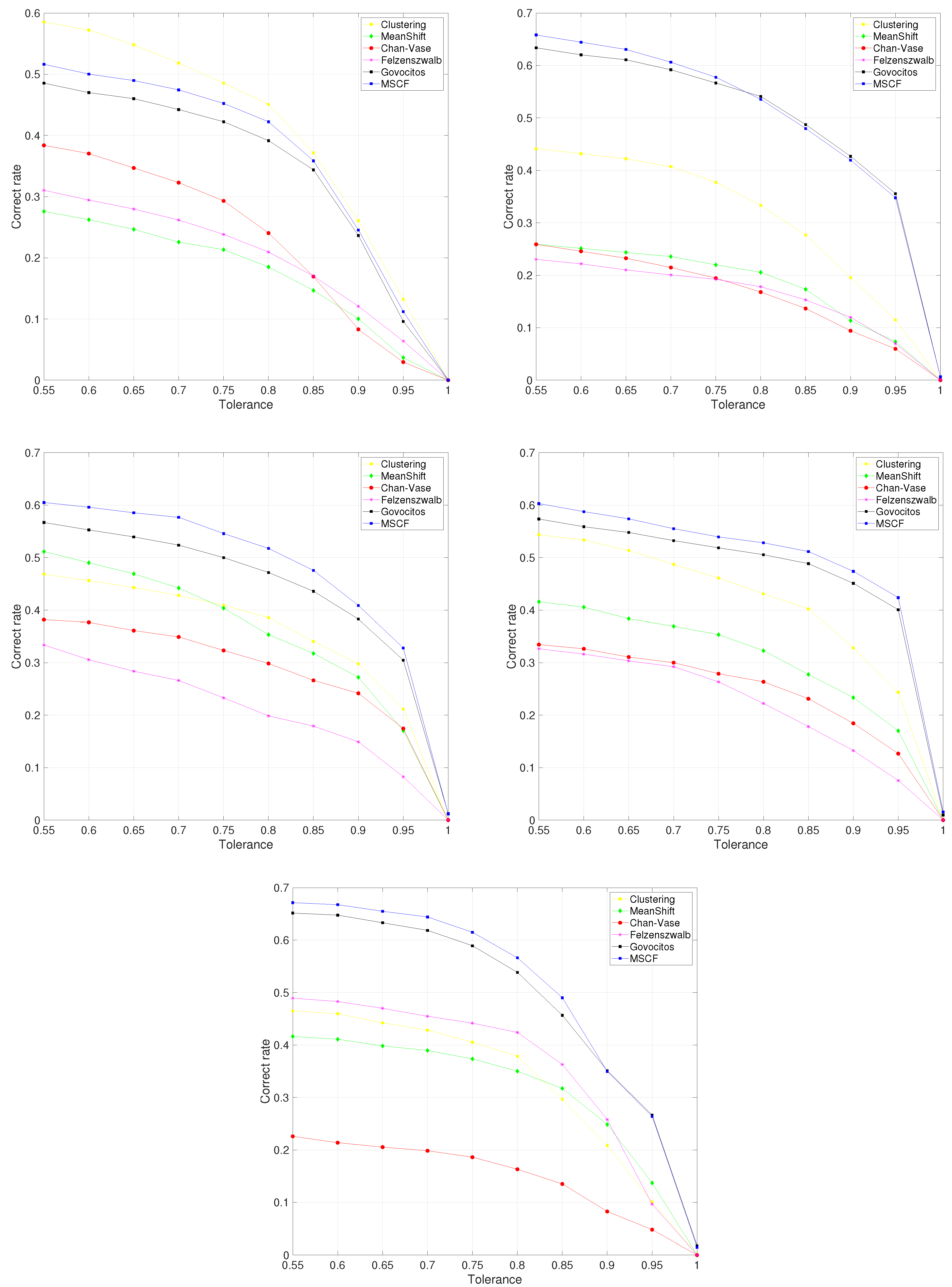Figure 2 shows the variation in correct cell recognition for different values of tolerance for all the fish species. The MSCF algorithm achieved the best results, followed by the Govocitos algorithm, with the exception of the European hake fish species, in which clustering provided the best results. The correct rate decreases as a stricter overlap between the computer-recognized and expert-annotated cell is required, i.e., for higher values of tolerance T, being practically zero when we demand a perfect cell overlap. Experts believe that an overlap of 70% could be acceptable for practical purposes. For this value, the average percentage of cells correctly recognized is 51.83% for the hake fish species and clustering segmentation algorithm, and 60.62%, 57.67%, 55.55% and 64.41% for the MSCF algorithm and the pouting, European pilchard, Four-spot and Roughhead grenadier species, respectively. The average performance for the different fish species ranges from 51.83% for European hake to 64.41% for Roughhead grenadier fish species. Figure 3 shows the performance of the MSCF algorithm using the best global configuration ($\mathcal{S}=\{2,4,6\}$ and $\mathcal{TH}=\left\{\right(0.55,0.75\left)\right\}$) for each image of all fish species. The left panel shows the correct cell recognition rate for a tolerance of T = 0.7 and the right panel presents the $F_1$ value. Among each fish species, there is great variability in performance in terms of the correct cell recognition rate and $F_1$ value. This behavior is similar for all fish species. It is important to emphasize that these datasets were built to test the robustness of the STERapp software, and the images present high variability. The absolute performance at a pixel level ($F_1$ value) is always higher than at the region level (correct cell recognition rate), which confirms the hypothesis that the pixels are correctly labeled as cells or background but the connectivity among pixels could not be correctly identified. Thus, we can conclude that the MSCF algorithm can be automatically run to recognize cells for some images but, for other images, the recognition of cells could be practically performed manually by the fishery experts. Thus, in order to provide a fully automatic tool to estimate fecundity, it will be necessary to adopt software like STERapp that combines automatic processing with an intuitive graphical interface to review the recognition results before image quantification [27].

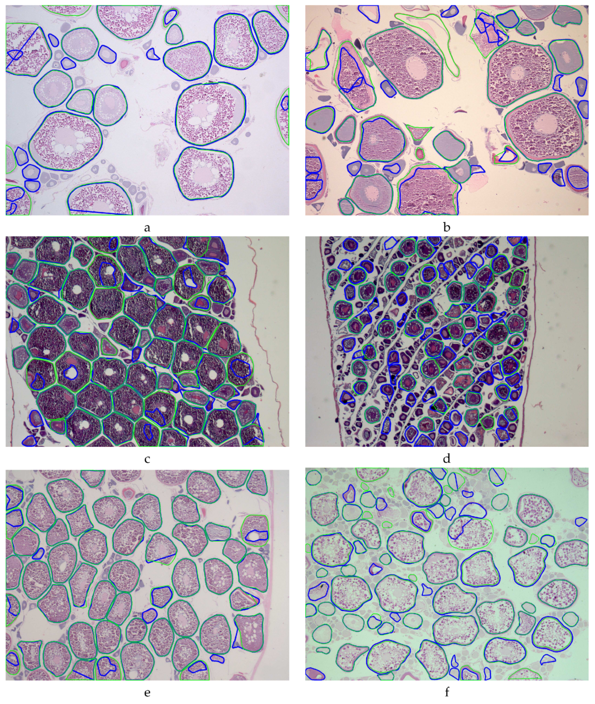
Figure 4 shows visual examples of the performance of the MSCF algorithm for the different fish species, where the cell contour annotated by the expert and the cell outline recognized by the algorithm are overlapped with the image in green and blue, respectively. In all cases, we use the minimum diameter $D_{min}=100$ pixels. As can be seen visually in the images, some false positive cells are due to the detection of cells whose sizes are between matured and immature. In some cases, they were detected by the algorithm, but the experts considered them immature. This fact led us to perform additional experiments using a greater $D_{min}$ value, providing slightly higher performance results. Thus, in the current version of STERapp [27], the process of cell recognition can be achieved using two steps: firstly using a larger diameter and, if it is necessary, using a second diameter to add the undetected cells.

To determine which is the best algorithm globally,

Table 5. Friedman ranking of the different segmentation algorithms using correct cell recognition as a quality measure and using $D_{\min }=100$.

Position	Rank	Algorithm
1	1.2	MSCF
2	2.2	Govocitos
3	3	Clustering
4	4.4	Meanshift
5	4.8	Felzenszwalb
6	5.4	Chan–Vese

shows the Friedman ranking of the algorithms over all datasets for correct cell recognition. The MSCF algorithm achieved the first position, very near to 1. This means that it achieved the best performance in almost all the experiments. The second position, with a ranking of 2.2 (i.e., the second-best performance in almost all the experiments), was achieved by Govocitos, followed by clustering, meanshift, Felzenszwalb and Chan–Vese in the last position.

All the experiments were performed on a computer equipped with 32 GB of RAM and a 3.10 GHz processor under Linux Kubuntu 20.04. The average elapsed time of the segmentation algorithms per image, using the configuration that provided the best performance for each fish species, was 4.61 s for clustering, 2.97 s for Felzenszwalb, 3.83 s for Govocitos, 2.69 s for MSCF, 133.31 s for meanshift and 165.04 s for the Chan–Vese algorithm. The MSCF algorithm was the fastest one, followed by Felzenszwalb, Govocitos and clustering. In fact, the time needed by the first four algorithms was only a few seconds, which makes them suitable for image processing in interactive applications, while the last two require more than one minute and they are too slow for real-time applications.

5. Conclusions

We propose a segmentation algorithm based on the Canny edge detector, called the multi-scale Canny filter (MSCF), to recognize cells in microscopic images. The classical Canny edge detector combines the following steps: (1) smoothing of the grey-level image using a $\sigma$-width Gaussian kernel; (2) differentiation using a first derivative operator; (3) performing the non-maxima suppression process, which finds local maxima in the direction perpendicular to the edge; and (4) performing thresholding with hysteresis. MSCF considers different scales using a set of $\sigma$ values, and the thresholds to the hysteresis process are selected automatically from the image characteristics. Finally, there is a fusion process of the information coming from different scales. Our approach has been statistically evaluated over five datasets of histological images of fish ovaries, providing $F_1$ values from 70% to 80% for the different fish species. Compared with other state-of-the-art segmentation techniques, MSCF globally achieved the highest performance both in pixel classification (the highest $F_1$ values) and cell recognition, measured as the percentage of cells correctly recognized for a level of overlapping tolerance. This percentage for the different fish species ranged from 51.83% for European hake to 64.41% for the Roughhead grenadier dataset. Globally, the MSCF algorithm achieved the first position using the Friedman ranking, followed by Govocitos, clustering, meanshift and Felzenszwalb, and the last one was the Chan–Vese method.

In conclusion, our MSCF algorithm is very competitive, both in computational time and performance, with other state-of-the-art segmentation algorithms. We verified that the problem of recognizing cells in histological images of fish gonads is very challenging, and that a completely automatic approach is still not available. Our future work will continue designing new approaches to solve automatically this problem.

References

1. Österblom, H.; Crona, B.I.; Folke, C.; Nyström, M.; Troell, M. Marine Ecosystem Science on an Intertwined Planet. Ecosystems 2017, 20, 54–61. [Google Scholar] [CrossRef]
2. Gebremedhin, S.; Bruneel, S.; Getahun, A.; Anteneh, W.; Goethals, P. Scientific Methods to Understand Fish Population Dynamics and Support Sustainable Fisheries Management. Water 2021, 13, 574. [Google Scholar] [CrossRef]
3. Trippel, E.A. Estimation of Stock Reproductive Potential: History and Challenges for Canadian Atlantic Gadoid Stock Assessments. J. Northwest Atl. Fish. Sci. 1999, 25, 61–81. [Google Scholar] [CrossRef]
4. Lasker, R. An Egg Production Method for Estimating Spawning Biomass of Pelagic Fish: Application to the Northern Anchovy, Engraulis mordax; Technical Report 36; U.S. Department of Commerce: Washington, DC, USA, 1985.
5. Hunter, J.R.; Macewicz, J.; Lo, N.C.H.; Kimbrell, C.A. Fecundity, spawning, and maturity of female Dover Sole, Microstomus pacificus, with an evaluation of assumptions and precision. Fish. Bull. 1992, 90, 101–128. [Google Scholar]
6. Ganias, K. Determining the indeterminate: Evolving concepts and methods on the assessment of the fecundity pattern of fishes. Fish. Res. 2013, 138, 23–30. [Google Scholar] [CrossRef]
7. Weibel, E.R.; Gómez, D.M. A principle for counting tissue structures on random sections. J. Appl. Physiol. 1962, 17, 343. [Google Scholar] [CrossRef]
8. Weibel, E.R. Steorological Method: Practical Methods for Biological Morphometry; Academic Press: Cambridge, MA, USA, 1979. [Google Scholar]
9. Emerson, L.S.; Greer-Walker, M.; Witthames, P.R. A stereological method for estimating fish fecundity. J. Fish Biol. 1990, 36, 721–730. [Google Scholar] [CrossRef]
10. Pintor, J.; Carrión, P.; Cernadas, E.; González-Rufino, E.; Formella, A.; Fernández-Delgado, M.; Domínguez-Petit, R.; Rábade-Uberos, S. Govocitos: A software tool for estimating fish fecundity based on digital analysis of histological images. Comput. Electr. Agric. 2016, 125, 89–98. [Google Scholar] [CrossRef]
11. González, R.C.; Woods, R.E. Digital Image Processing, 3rd ed.; Pearson Prentice Hall: Hoboken, NJ, USA, 2008. [Google Scholar]
12. Cremers, D.; Rousson, M.; Direche, R. A Review of Statistical Aproached to Level Set Segmentation: Integrating Color, Texture, Motion and Shape. Int. J. Comput. Vis. 2007, 72, 195–215. [Google Scholar] [CrossRef]
13. Peng, B.; Zhang, L.; Zhang, D. A survey of graph theoretical approaches to image segmentation. Pattern Recogn. 2013, 42, 1020–1038. [Google Scholar] [CrossRef]
14. Canny, J.F. A computational approach to edge detection. IEEE Trans. Pattern Anal. Mach. Intell. 1986, 8, 679–698. [Google Scholar] [CrossRef] [PubMed]
15. Chan, T.; Vese, L. Active Contours without Edges. IEEE Trans. Image Process. 2001, 10, 266–277. [Google Scholar] [CrossRef]
16. Shi, J.; Malik, J. Normalized Cuts and Image Segmentation. IEEE Trans. Pattern Anal. Mach. Intell. 2000, 22, 888–905. [Google Scholar]
17. Felzenszwalb, P.F.; Huttenlocher, D.P. Efficient Graph-Based Image Segmentation. Int. J. Comput. Vis. 2004, 59, 167–181. [Google Scholar] [CrossRef]
18. Comaniciu, D.; Meer, P. Mean Shift: A Robust Approach Toward Feature Space Analysis. IEEE Trans. Pattern Anal. Mach. Intell. 2002, 24, 603–619. [Google Scholar] [CrossRef]
19. Atienza, R. Advanced Deep Learning with TensorFlow 2 and Keras: Apply DL, GANs, VAEs, Deep RL, Unsupervised Learning, Object Detection and Segmentation, and More, 2nd ed.; Packt Publishing: Birmingham, UK, 2020. [Google Scholar]
20. Liu, X.; Song, L.; Liu, S.; Zhang, Y. A Review of Deep-Learning-Based Medical Image Segmentation Methods. Sustainability 2021, 13, 1224. [Google Scholar] [CrossRef]
21. Jiang, H.; Zhou, Y.; Lin, Y.; Chan, R.C.; Liu, J.; Chen, H. Deep learning for computational cytology: A survey. Med. Image Anal. 2023, 84, 102691. [Google Scholar] [CrossRef]
22. Deng, S.; Zhang, X.; Yan, W.; Chang, E.I.C.; Fan, Y.; Lai, M.; Xu, Y. Deep learning in digital pathology image analysis: A survey. Front. Med. 2020, 14, 470–487. [Google Scholar] [CrossRef]
23. Long, F. Microscopy cell nuclei segmentation with enhanced U-Net. BMC Bioinform. 2020, 21, 8. [Google Scholar] [CrossRef]
24. Chen, L.C.; Papandreou, G.; Kokkinos, I.; Murphy, K.; Yuille, A.L. DeepLab: Semantic Image Segmentation with Deep Convolutional Nets, Atrous Convolution, and Fully Connected CRFs. IEEE Trans. Pattern Anal. Mach. Intell. 2018, 40, 834–848. [Google Scholar] [CrossRef]
25. Badrinarayanan, V.; Kendall, A.; Cipolla, R. SegNet: A Deep Convolutional Encoder-Decoder Architecture for Image Segmentation. IEEE Trans. Pattern Anal. Mach. Intell. 2017, 39, 2481–2495. [Google Scholar] [CrossRef] [PubMed]
26. Mbaidin, A.; Rábade-Uberos, S.; Dominguez-Petit, R.; Villaverde, A.; Gónzalez-Rufino, M.E.; Formella, A.; Fernández-Delgado, M.; Cernadas, E. STERapp: Semiautomatic Software for Stereological Analysis. Application in the Estimation of Fish Fecundity. Electronics 2021, 10, 1432. [Google Scholar] [CrossRef]
27. Mbaidin, A.; Cernadas, E.; Al-Tarawneh, Z.; Fernández-Delgado, M. Recognizing cells in histological images of fish gonads. In Proceedings of the 2022 International Conference on Emerging Trends in Computing and Engineering Applications (ETCEA), Karak, Jordan, 23–24 November 2022; pp. 1–6. [Google Scholar] [CrossRef]
28. Medina-Carnicer, R.; Muñoz-Salinas, R.; Yeguas-Bolivar, E.; Diaz-Mas, L. A novel method to look for the hysteresis thresholds for the Canny edge detector. Pattern Recogn. 2011, 44, 1201–1211. [Google Scholar] [CrossRef]
29. Sheskin, D. Handbook of Parametric and Nonparametric Statistical Procedures; Chapman and Hall/CRC Press: Boca Raton, FL, USA, 2006. [Google Scholar]
30. Getreuer, P. Chan-Vese Segmentation. Image Process. On Line 2012, 2, 214–224. [Google Scholar] [CrossRef]
31. Suzuki, S.; Be, K. Topological structural analysis of digitized binary images by border following. Comput. Vis. Graph. 1985, 30, 32–46. [Google Scholar] [CrossRef]
32. Ojala, T.; Piatikäinen, M.; Mäenpää, T. Multiresolution grey-scale and rotation invariant texture 66 classification with Local Binary Pattern. IEEE Trans. Patt. Anal. 2002, 24, 971–987. [Google Scholar] [CrossRef]
33. Varma, M.; Zisserman, A. A statistical approach to material classification using image patch 68 exemplars. IEEE Trans. Patt. Anal. 2009, 31, 2032–2047. [Google Scholar] [CrossRef]
Figure 1. Examples of histological images of European hake (a), Trisopterus luscus (b), European pilchard (c), Four-spot megrim (d) and Roughhead grenadier (e,f) fish species with the outline of the ground truth cells overlapped. Different colors reflect different development stages of matured cells.
Sustainability 15 13693 g001
Figure 2. Correct rate of cell recognition for different values of tolerance and fish species, European hake (upper left), Trisopterus luscus (upper right), European pilchard (midle left), Four-spot megrim (middle right) and Roughhead grenadier (lower), achieved by the tested segmentation algorithms using the minimum cell diameter D m i n = 100 pixels.
Sustainability 15 13693 g002
Figure 3. Correct rate of cell recognition for different values of tolerance and Roughhead grenadier species achieved by the tested segmentation algorithms using the minimum cell diameter D m i n = 100 pixels (left panel). The right panel shows the correct cell recognition rate achieved by the MSCF algorithm for each image of all the fish species.
Sustainability 15 13693 g003
Figure 4. Examples of histological images of European hake (a), Trisopterus luscus (b), European pilchard (c,d), Four-spot megrim (e) and Roughhead grenadier (f) fish species with the outline of the ground truth cells (in green color) and computer-recognized cells (in blue color) overlapped.
Sustainability 15 13693 g004