Creating Rutting Prediction Models through Machine Learning Techniques Utilizing the Long-Term Pavement Performance Database

Abstract

Over time, roads undergo deterioration caused by various factors such as traffic loads, climate conditions, and material properties. Considering the substantial global investments in road construction, it is crucial to periodically assess and implement maintenance and rehabilitation (M and R) plans to ensure the network’s acceptable level of service. An integral component of the M and R plan involves utilizing performance prediction models, especially for rutting distress, a significant issue in asphalt pavement. This study aimed to develop rutting prediction models using data from the Long-Term Pavement Performance (LTPP) database, employing several machine learning techniques such as regression tree (RT), support vector machine (SVM), ensembles, Gaussian process regression (GPR), and Artificial Neural Network (ANN). These techniques are well-known for effectively handling extensive and complex datasets. To achieve the highest modeling accuracy, the parameters of each model were meticulously fine-tuned. Upon evaluation, the results revealed that the GPR models outperformed other techniques in various metrics, including Root Mean Square Error (RMSE), R-squared, Mean Absolute Error (MAE), and Mean Square Error (MSE). The best GPR model achieved an RMSE of 1.96, R-squared of 0.70, MAE of 1.32, and MSE of 109.33, indicating its superior predictive capabilities compared with the other machine learning methods tested in this study. Comparison Analysis was made for 10 randomly selected sections on our novel machine learning model that outperforms existing models, with an R² of 0.989 compared with 0.303 and 0.3095 for other models. This demonstrates the potential of advanced machine learning in accurate rut depth prediction across diverse climates, aiding pavement management decisions.

1. Introduction

A country’s economic prosperity heavily relies on a well-maintained transportation infrastructure [1]. However, in the United States (US), more than 21% of pavements are in poor condition, while the available annual funding for maintenance and improvements only covers about 60% of the required budget due to financial constraints [2,3]. Recognizing the importance of strategic and cost-effective pavement maintenance and rehabilitation approaches, governments and highway agencies are increasingly relying on efficient pavement management systems (PMS). Pavements play a critical role in the transportation network, directly encountering vehicle loads and transferring them to road subgrades, providing a safe and stable platform for vehicle movement. Keeping pavements in good condition not only protects a nation’s assets but also enhances transit safety and comfort. Predicting pavement behavior throughout its lifecycle is crucial to ensure timely repairs and reduce maintenance costs. By developing reliable distress/performance prediction models, the heart of the PMS system, the rate of pavement deterioration can be quantified, and maintenance and rehabilitation operations can be defined in a cost-effective and budget-supported manner [4,5,6]. This approach aligns with the primary objective of the PMS, which aims to establish the most efficient policies for M and R operations. Implementing such predictive models empowers transportation authorities to create a secure transit network while optimizing expenses related to maintenance and rehabilitation activities.

Rutting, also known as permanent deformation, poses a significant challenge for asphalt pavements, often resulting in structural failure within the pavement layers. This distress occurs due to vertical compressive strain on the subgrade layer caused by underlying foundation weaknesses [7]. The accumulation of non-recoverable deformation is primarily induced by repetitive loads, particularly under elevated temperatures. As a consequence, rutting adversely impacts road safety, service life, and maintenance costs [8,9,10,11,12].

Over time, various pavement distress prediction models have been developed, each possessing distinct characteristics in terms of generality, accuracy in estimating pavement performance, and data requirements. Empirical models are commonly specific to certain traffic and weather conditions, while mechanistic-empirical models combine mechanistic approaches to estimate input parameters [13]. A performance prediction model is a mathematical tool that forecasts future pavement deterioration based on the current condition of the pavement and other relevant influencing factors [14]. Historical data concerning pavement condition, age, and traffic play a vital role in the development of such predictive models. These models serve as a fundamental resource for effective pavement management systems (PMS) [14]. However, pavement distress prediction models are highly effective in fundamental decision-making processes, offering answers to questions about what, where, and when maintenance demands should be addressed. These models play a crucial role in devising a timely M and R strategy, and determining when to initiate an action plan to maintain the road network at an acceptable level of service [15]. By employing these models, highway agencies can optimize their maintenance efforts and ensure the road infrastructure operates efficiently and safely.

The Long-Term Pavement Program (LTPP) was established in 1987 as a component of the Strategic Highway Research Program (SHRP). Its main objective is to build a comprehensive nationwide long-term pavement database that supports the objectives of SHRP and meets future research needs [16]. The LTPP database contains meticulously collected information from approximately 2500 pavement sections, spanning 30 years. This data includes details about pavement construction, structure, material properties, maintenance and rehabilitation activities, pavement condition, load-bearing capacity, and environmental conditions. The wealth of information in the LTPP database allows for the creation of baseline deterioration prediction models, which serve as the foundation for developing effective Pavement Management Systems (PMS) in any state. These baseline models can be adapted and modified based on the specific experiences and data of individual highway agencies. Additionally, the LTPP data plays a crucial role in the calibration of Mechanistic-Empirical Pavement Design Guide (MEPDG) models [17]. The calibration process ensures that the MEPDG models are accurate and reliable, allowing for more precise pavement design and management decisions. Overall, the LTPP database is an invaluable resource for advancing pavement engineering research, contributing to better-designed road networks, and enhancing the longevity and performance of transportation infrastructure.

To formulate accurate and effective rutting prediction models, significant efforts have been dedicated over the past few decades. A straightforward approach involves the utilization of empirical models to forecast rutting performance. This method typically establishes a conventional linear or nonlinear function that correlates rutting depth with parameters such as pavement structure, materials, climate, and traffic characteristics [18,19,20,21,22]. For instance, Abu-Ennab [18] employed a simple linear regression to predict rutting depth based on pavement age, yet the model’s coefficient of determination (R2) remained below 0.1. George [19] applied a power regression model that considered age and traffic inputs derived from three years of pavement condition data, yielding an R2 value of 0.68. Among the commonly used empirical rutting prediction models is the Asphalt Institute model [23], which establishes connections between rut depth and factors like traffic volume, axle load, and pavement thickness. Another example is the Shell model, which factors in traffic loads and environmental conditions. However, empirical rutting prediction models exhibit several limitations.

Firstly, empirical models lack the incorporation of underlying mechanistic behaviors within pavement layers and their interactions [24]. These result in a deficiency of insights into how different factors contribute to rutting, thereby limiting the model’s ability to capture intricate variations. Secondly, empirical models are often constructed based on specific datasets and conditions [25]. Extrapolating these models to diverse regions, climates, or materials can lead to inaccuracies due to unaccounted variations present in the original dataset. Thirdly, empirical models can be sensitive to outliers and anomalies in the data [26]. Atypical or extreme data points might disproportionately impact the model’s predictions, causing inaccuracies. Fourthly, empirical models might struggle to adapt to changing conditions, such as alterations in traffic patterns, material properties, or climate [25]. This lack of adaptability can lead to inaccuracies in long-term rutting predictions. Lastly, empirical models might encounter difficulties in predicting rutting for novel pavement materials that have not been extensively studied and incorporated into the model’s developmental dataset [26].

In contrast, mechanistic models involve the computation of permanent deformation accumulation, integrating specific material behaviors like the viscoplastic model [27] and the elastic-viscoplastic model [28]. These models operate within diverse loading conditions such as pulse loads [27], moving loads [29], and equivalent loads [30], utilizing methods like finite element [31] and discrete element approaches [32]. However, simulating actual loading and varying climate conditions presents challenges due to the complexity of tire-pavement contact areas and stress distribution. Additionally, numerical simulations for just one cycle can consume significant time, ranging from hours to days.

In 2004, the Mechanistic-Empirical Pavement Design Guide (MEPDG) was introduced, presenting a mechanistic-empirical (M-E) approach to rutting prediction [31]. The M-E method involves establishing a regression equation linking rutting depth to factors including pavement structural responses, climate conditions, traffic loadings, material properties, and wheel tracking test outcomes. The application of MEPDG’s rutting prediction model necessitates the acquisition of local calibration factors. Researchers such as Sun et al. [33], Darter et al. [34], Kaya [35], and Mellela et al. [36] have calibrated rutting prediction models for specific regions (Kansas, Arizona, Iowa, and Ohio), with achieved R2 values of 0.24, 0.18, 0.63, and 0.63, respectively. These models notably exhibit subpar performances. Moreover, the mechanistic elements of these models entail complex calculations and simulations to forecast pavement responses under various loading conditions [37,38]. This complexity results in substantial computational demands, necessitating specialized software and computational resources. Mechanistic-empirical models mandate rigorous calibration and validation using local data to ensure their precision for specific regions or conditions [39]. Incorrect calibration can lead to unreliable predictions.

In recent years, numerous research endeavors have explored the application of computational intelligence-based methodologies as an alternative to overcome the limitations of performance prediction models reliant on empirical predictive equations. Among these efforts, neural networks have demonstrated superiority in predicting pavement roughness compared with classical predictive models [39,40,41,42]. Furthermore, in the realm of pavement distress prediction, neural networks have been utilized to forecast the progression of cracked regions over time [43] and to identify the initiation of fatigue cracking [44]. These neural network-based approaches have proven to be effective in capturing complex patterns and relationships within the data, allowing for more accurate and reliable predictions of pavement deterioration and distress. Despite the widespread application of machine learning in various fields for pavement performance, there is a paucity of studies utilizing machine learning algorithms for predicting rutting in asphalt pavement using LTPP data [45]. Also, the full potential of the Long-Term Pavement Performance dataset, which includes comprehensive information on pavement performance and rutting measurements, remains largely untapped in the context of developing accurate rutting prediction models using machine learning techniques [46]. The nature of the LTPP database is quite complicated to model using traditional statistical methods, which requires more advanced techniques such as ML and ANN. Existing rutting prediction models rely on traditional statistical approaches or simplified empirical equations, which may not adequately capture the complexity of factors influencing rutting in asphalt pavement. Further research is needed to develop comprehensive predictive models using machine learning algorithms [47]. The central aim of this study is to perform a comparative examination of five artificial intelligence and machine learning techniques used for predicting rutting in asphalt pavements. The chosen methodologies under investigation encompass regression decision trees, Support Vector Machines (SVMs), ensemble trees (both bagged and boosted), Gaussian Process Regression (GPR), and Artificial Neural Networks (ANN).

2. Research Objectives

The primary objective of this research study is to conduct a comparative analysis of five AI/ML approaches for predicting rutting in asphalt pavements. The selected methods for investigation are regression decision tree, Support Vector Machine (SVM), ensemble tree (bagged and boosted), Gaussian Process Regression (GPR), and Artificial Neural Networks (ANN). To achieve this goal, data has been extracted from the comprehensive Long-Term Pavement Performance (LTPP) database, which provides a wealth of time series and variable information. The specific objectives of the study can be summarized as follows:

• Investigate the data: perform a thorough analysis of the dataset by computing descriptive statistics to gain insights into the characteristics of the collected data.
• Explore rutting’s relationship with independent design factors: examine the correlations between rutting, the main dependent variable, and all the other scalar independent design factors (features) to identify potential relationships and patterns.
• Develop rutting prediction models: utilize multiple machine learning techniques to create robust rutting prediction models using the data extracted from the LTPP database.
• Optimize model performance: fine-tune the parameters of the chosen AI/ML models to enhance their prediction accuracy and overall performance.
• Compare model performance: Conduct a comparative analysis of the developed rutting prediction models, evaluating their prediction accuracy and model training time. This comparison aims to identify which model performs best for the specific task.
• Identify influential factors: Determine the relative impact of different factors on rutting prediction. This analysis will help in understanding which design factors play a significant role in influencing the rutting behavior in asphalt pavements.
• To compare the performance of the newly developed machine learning model with existing empirical models in predicting rut depth for different climate zones, providing valuable insights into the model’s accuracy and reliability.

3. Methodology

The research study followed a structured methodology comprising several stages, as presented in Figure 1. Initially, data retrieval involved extracting asphalt pavement control sections from both cold and warm climate zones, resulting in a selection of 425 sections encompassing diverse climatic conditions. Subsequently, the raw data underwent processing, integration, and cleaning to ensure its suitability for exploration, visualization, and modeling. For this study, rutting was adopted as the pavement performance indicator, serving as the main dependent variable for analysis. The study also aimed to explore the relationship between rutting and all other independent variables (features) to detect any notable patterns. State-of-the-art machine learning models were then employed to develop highly effective rutting prediction models. Given the uncertainty regarding the optimal machine learning technique for modeling rutting, the study recommended the use of multiple techniques. As a result, five state-of-the-art machine learning techniques were chosen: regression tree (RT), support vector machine (SVM), ensembles, Gaussian process regression (GPR), and Artificial Neural Network (ANN). Further details on these five techniques will be elaborated below.

To ensure a robust and comprehensive analysis, our methodology includes the use of both the complete input set and a selected subset of variables derived from variable importance analysis. This dual approach serves several purposes:

• Benchmarking and Validation: By comparing predictive outcomes between the two scenarios, we validate the effectiveness of our variable selection process and quantify improvements achieved through identifying key variables.
• Robustness Testing: The comprehensive analysis aids in evaluating the model’s performance across different input configurations, ensuring its robustness and generalization capabilities.
• Variable Importance and Stability: Consistency between outcomes validate variable importance rankings and assures model stability, lending credibility to identified key variables.

It is important to note that the data preprocessing, filtering, visualization, and modeling stages were carried out using a combination of Microsoft Excel©, Microsoft Access©, and MATLAB©.

4. Data Description and Preprocessing

The data utilized for the proposed analysis was sourced from the Long-Term Pavement Performance (LTPP) database. The establishment of the LTPP database dates back to 1987, with the primary objective of investigating methods to construct high-performing pavements under diverse conditions. The database encompasses data collected from over 600 pavement sections and includes archival data from more than 1900 pavement sections. The data collection conducted by the LTPP involves two main schemes: general pavement studies and specific pavement studies (SPS) [48]. The LTPP is overseen and operated by the Federal Highway Administration (FHWA), which also takes responsibility for providing free access to the data on its website, accessible at https://infopave.fhwa.dot.gov/ (accessed on 22 July 2023). Researchers and professionals in the field of pavement engineering can utilize this valuable repository of data to support their analyses and studies.

For this research study, control asphalt pavement sections situated in both cold and warm climate regions, with and without freezing conditions, and having no history of maintenance or rehabilitation activities were extracted from the LTPP database. The data selection process resulted in a total of 420 control pavement sections, encompassing 1584 individual records that met these specific criteria. Four primary data types were retrieved from the LTPP database, including structure, climate, traffic, and performance-related information.

Table 1. Summary of the collected data.

Data Type	Data Attribute	Description	Number/Categorical
Structure	Age (years)	The age of the pavement structure in years since its construction.	Number
	Construction Number	A unique identifier for each construction project or phase.	Number
	Layer #1 Material Description	Description of the material used in the topmost layer of the pavement.	Categorical
	Layer #2 Type	Type of material used in the second layer of the pavement.	Categorical
	Layer #2 Thickness (mm)	Thickness of the second layer of the pavement in millimeters.	Number
	Layer #2 Material Description	Description of the material used in the second layer of the pavement.	Categorical
	Layer #3 Type	Type of material used in the third layer of the pavement.	Categorical
	Layer #3 Thickness (mm)	Thickness of the third layer of the pavement in millimeters.	Number
	Layer #3 Material Description	Description of the material used in the third layer of the pavement.	Categorical
	Layer #4 Type	Type of material used in the fourth layer of the pavement.	Categorical
	Layer #4 Thickness (mm)	Thickness of the fourth layer of the pavement in millimeters.	Number
	Layer #4 Material Description	Description of the material used in the fourth layer of the pavement.	Categorical
	Drainage Type	Type of drainage system used for the pavement.	Categorical
	Drainage Location	Location of the drainage system in relation to the pavement layers.	Categorical
	Resilient Modulus of Layer #2 (MPa)	Resilient modulus of the second layer of the pavement, which represents its ability to withstand deformation under load.	Number
	Resilient Modulus of Layer #3 (MPa)	Resilient modulus of the third layer of the pavement.	Number
	Resilient Modulus of Layer #4 (MPa)	Resilient modulus of the fourth layer of the pavement.	Number
Climate	Climate Zone	Classification of the geographical area based on climate characteristics.	Categorical
	Annual Average Precipitation (mm)	Average amount of rainfall in millimeters experienced over a year.	Number
	Annual Average Temperature (deg C)	Average temperature in degrees Celsius experienced over a year.	Number
	Annual Average Freeze Index (deg C deg days)	Index that represents the severity and duration of freezing conditions.	Number
	Min Relative Humidity (%)	Lowest relative humidity level recorded.	Number
	Max Relative Humidity (%)	Highest relative humidity level recorded.	Number
	Annual Average Relative Humidity (%)	Average relative humidity experienced over a year.	Number
	Annual Average Wind Velocity (m/s)	Average wind speed in meters per second experienced over a year.	Number
	Max Annual Average Wind Velocity (m/s)	Maximum wind speed in meters per second experienced over a year.	Number
Traffic	Number of Lanes	The total number of lanes in the road.	Categorical
	ESALs	Equivalent Single Axle Loads, a measure of the impact of traffic loads on the pavement.	Number
	Annual Average Daily Truck Traffic (AADTT)	Average number of trucks passing a certain point on the road daily.	Number
Performance	Initial IRI (m/km)	International Roughness Index, a measure of pavement roughness.	Number
	Rutting (mm)	Rutting depth, a measure of pavement deformation caused by traffic loads.	Number

presents the chosen attributes within each category, outlining the specific variables used in the analysis. The variables collected are Age (#years), Construction Number (distinguish different pavement sections within the LTPP database), Layer Material Description (materials used in the construction of a specific pavement section or project), Layer Type(composition of each layer within a pavement section), Layer Thickness (depth of each individual layer within a pavement section), drainage type (strategies and elements implemented to ensure effective water management within the pavement structure), drainage location (where drainage features are positioned relative to the pavement structure), resilient modulus (mechanical property that characterizes the material’s stiffness), climate zone (categorization of geographical areas based on their specific climate characteristics and conditions), Annual Average Precipitation, Annual Average Temperature, Annual Average Temperature, Annual Average Freeze Index, Annual Average Relative Humidity, Annual Average Wind Velocity, Max Annual Average Wind Velocity, Number of Lanes, ESALs (is a unit of measurement used to quantify the cumulative effect of axle loads from various types of vehicles on a pavement over time), and Annual Average Daily Truck Traffic.

The inputs were chosen based on the parameters that are likely to affect rutting as defined by usual pavement engineering practice and the findings of the literature studies. Features that do not require sophisticated testing and are easily accessible in data-scarce areas were examined. Data availability was also taken into account during the selection process, as a big dataset is required for training machine learning models. This resulted in a set of 35 input variables reflecting climate and traffic conditions, material, and structural qualities.

The selection of input variables for predicting rutting depth in asphalt pavements is rooted in their direct or indirect influence on creating and developing this type of pavement distress. Each variable reflects specific attributes of the pavement structure, environmental conditions, and traffic loads, which collectively contribute to the phenomenon of rutting. The age of the pavement (Age) plays a crucial role in rutting development. Over time, the aging process causes degradation of the pavement materials, reducing their load-bearing capacity and leading to increased susceptibility to rutting. The deterioration is exacerbated by the accumulation of traffic-induced stresses, particularly in areas with higher traffic loads, such as the wheel paths. The layers of the pavement (Layer #1–4 Type and Thickness) define the composition and thickness of the pavement structure. These factors influence stress distribution across the layers, leading to differential settlements and localized stress concentrations. Pavements with thinner or weaker layers are more prone to rutting, as they exhibit decreased resistance to deformation under traffic loads.

The resilient modulus (Resilient Modulus of Layer #2–4) of the pavement layers is a fundamental indicator of their stiffness and load-bearing capacity. Lower resilient moduli signify a reduced ability to distribute and dissipate stress, making the pavement more susceptible to permanent deformation, including rutting. Climate conditions, represented by variables such as annual average precipitation, temperature, and freeze index, play a significant role in rutting development. Cold climates with freeze–thaw cycles induce moisture-related distress, weakening the pavement structure and exacerbating rutting, especially in areas where moisture can penetrate and cause material degradation. Traffic parameters, such as traffic volume (ESALs) and annual average daily truck traffic (AADTT), directly impact pavement performance. Higher traffic loads generate more stress, particularly in the wheel paths where the load is concentrated. As a result, rutting tends to occur more rapidly in these regions.

Categorical attributes, like “Climate Region”, were essential in our analysis. We utilized a numerical mapping approach to convert these categories into meaningful values. For example, “Climate Region” categories were transformed into numerical representations: Dry Freeze as 1; Dry No-Freeze as 2; Wet Freeze as 3; Wet No-Freeze as 4. This method allowed our machine learning algorithms to interpret categorical information effectively while maintaining the integrity of the original data. By implementing this encoding strategy, we ensured that categorical attributes were appropriately processed during our analysis, contributing to the accuracy and reliability of our predictive models.

Construction Number (CN) was included as one of the input variables in the analysis. While CN may not exhibit a direct, one-to-one relationship with rutting depth, its inclusion is based on a conceptual rationale deeply rooted in pavement engineering.

5. Preliminary Analysis, Data Visualization, and Attribute Selection

To visually represent the chosen LTPP pavement sections, the geographic locations of the 425 sections were plotted on a map, categorizing them according to their respective states (see Figure 2). A descriptive statistical summary of the retrieved features from the database is presented in

Table 2. Statistical summary of the numeric variables.

Variable	Mean	Standard Deviation	Minimum	Maximum	25th Percentile	50th Percentile	75th Percentile
Rutting (mm)	6.17	3.88	0.00	29.00	3.60	5.50	8.00
Age (years)	11.82	8.83	0.00	50.00	5.00	9.00	17.00
Layer #2 Thickness (mm)	227.62	179.69	0.00	686.00	152.00	206.00	289.50
Layer #3 Thickness (mm)	138.57	89.89	3.00	538.00	74.00	119.00	196.00
Layer #4 Thickness (mm)	83.92	63.09	1.00	315.00	43.00	64.00	104.00
Annual Average Precipitation (mm)	1006.14	478.07	51.30	3708.80	714.90	1050.50	1304.70
Annual Average Temperature (°C)	14.01	6.03	−0.10	25.50	8.80	15.70	17.70
Annual Average Freeze Index	279.03	436.03	0.00	2397.00	0.00	33.00	366.85
Min Humidity (%)	18.69	10.60	2.00	51.00	11.00	19.00	25.50
Max Humidity (%)	114.73	6.54	87.00	140.00	112.00	115.00	118.00
Annual Average Humidity (%)	66.71	5.92	51.00	81.50	63.50	67.50	71.00
Annual Average Daily Truck Traffic (AADTT)	588.26	595.87	0.00	5336.00	128.00	436.00	845.00
18-kip ESAL	229.84	258.64	0.00	2347.00	91.50	150.00	262.00
Initial IRI	1.03	0.37	0.56	3.00	0.77	0.93	1.20
Annual Average Wind velocity (m/s)	3.78	0.83	1.50	7.80	3.30	3.70	4.20
Max Annual Average Wind Velocity (m/s)	24.27	5.24	3.63	50.00	21.00	23.70	26.80
Resilient Modulus of Layer #2 (MPa)	4.86	1.10	1.00	6.00	4.00	5.00	6.00
Resilient Modulus of Layer #3 (Mpa)	2.73	1.76	1.00	6.00	1.00	3.00	5.00
Resilient Modulus of Layer #4 Subbase (Mpa)	1.50	1.09	1.00	5.00	1.00	1.00	1.00
Layer #3 Avg Air Voids (wheel path)	6.96	4.18	0.92	27.92	4.30	6.18	8.04
Layer #3 Avg Air Voids (non-wheel path)	6.64	2.59	1.86	19.67	4.90	6.90	7.96
Layer #4 Avg Air Voids (wheel path)	6.48	3.59	1.44	22.06	3.99	6.28	8.04
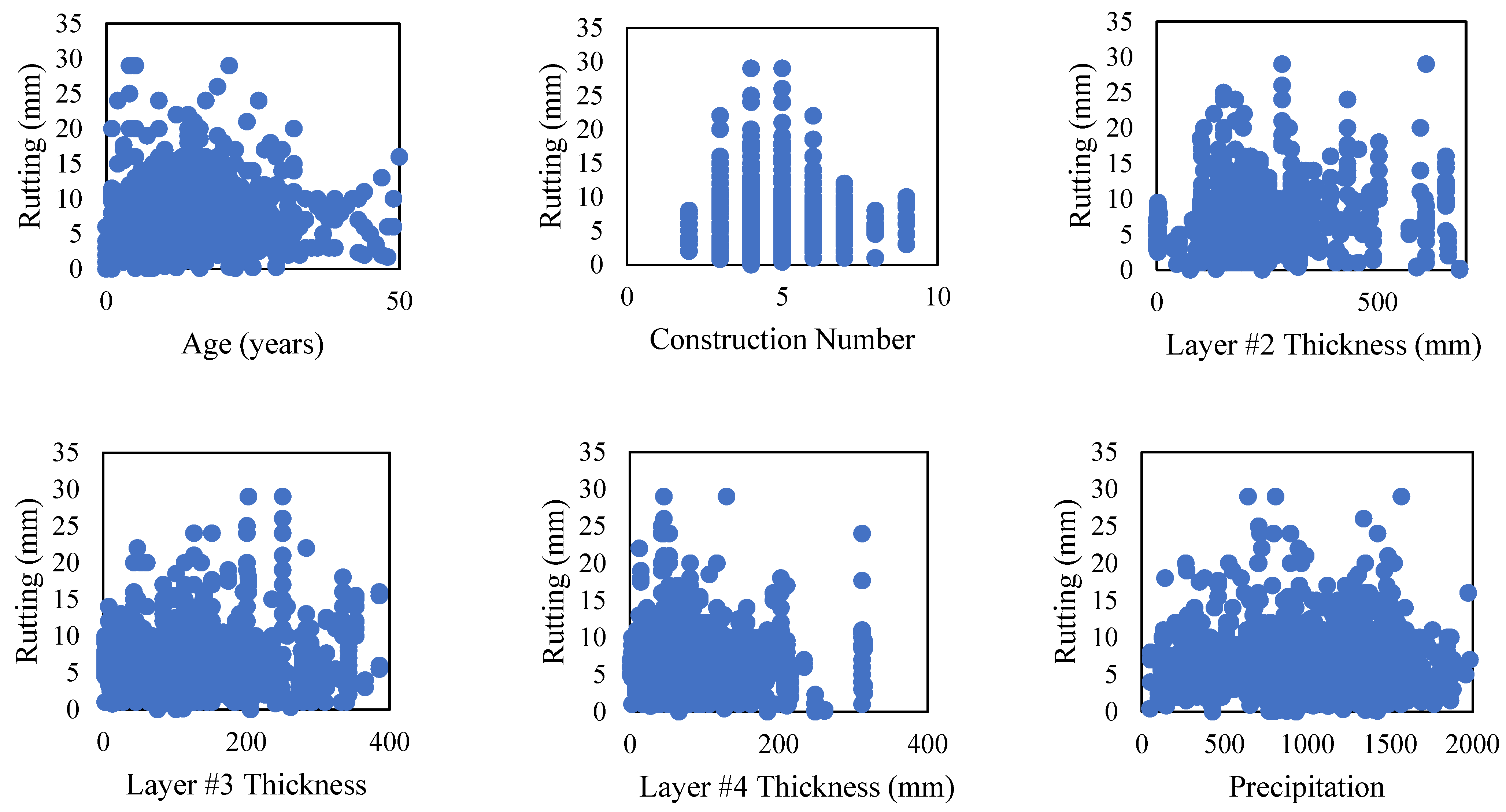
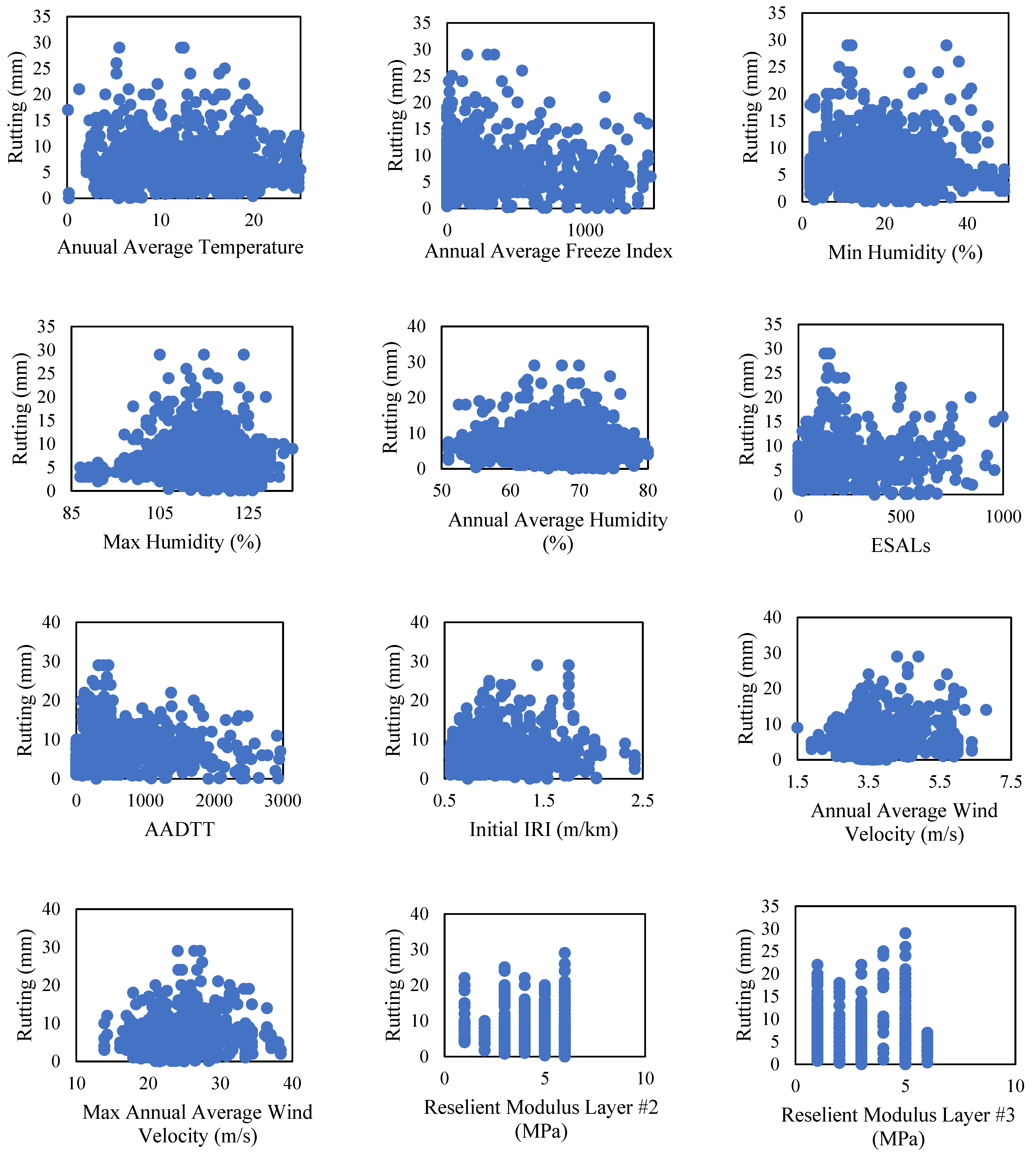
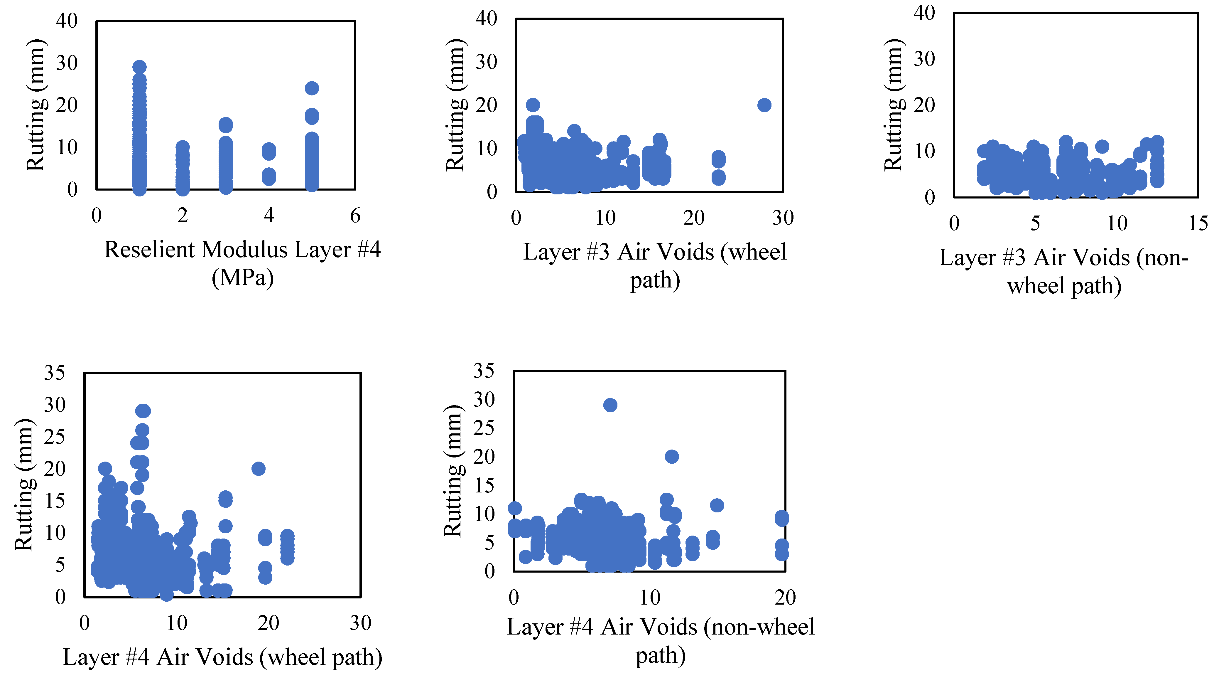
Layer #4 Avg Air Voids (non-wheel path)	6.86	3.17	0.08	19.76	4.94	6.55	8.14

. Additionally, the relationship between rutting (the primary dependent variable) and all the other independent design factors (features) was analyzed to identify any notable trends (see Figure 3). Figure 3 indicates that there are no easily discernible patterns between rutting and the other independent design factors. This suggests that conventional modeling techniques, such as linear regression, may not be sufficient to accurately model and investigate such relationships. Consequently, machine learning modeling techniques, which do not require pre-defined functional forms, appear to be a promising alternative.

The Weka Software 3.8.6 was utilized to assess the strength of the relationships between the independent variables and the dependent variable, rutting. Identifying the most correlated attributes to rutting and understanding their impact on rutting is crucial. This stage reveals the average correlation of attributes with rutting, aiding in the identification and removal of attributes with low correlation. This process aims to enhance result accuracy and reduce the number of inputs with similar model accuracy levels.

During this step, the “CorrelationAttributeEval” filter is applied to assess the correlation between rutting and other attributes. This process is vital as it aims to identify the attributes that have the strongest influence on rutting while disregarding less relevant attributes from the model. The “CorrelationAttributeEval” algorithm evaluates the significance of each attribute by measuring its correlation with rutting. The CorrelationAttributeEval algorithm is a feature selection technique that aims to assess the relationship between input attributes and a target variable, such as the rutting depth in our pavement distress prediction study. The algorithm operates through a systematic process that involves calculating correlations and ranking attributes based on their relevance to the target variable.

• Attribute Correlation Calculation: The algorithm starts by calculating the correlation coefficient between each input attribute and the target variable (rutting depth). The correlation coefficient measures the strength and direction of the linear relationship between two variables. A positive correlation indicates that higher values of one attribute are associated with higher values of rutting depth, while a negative correlation implies an inverse relationship.
• Average Merit Calculation: The calculated correlation coefficients for each attribute and rutting depth are then averaged to obtain the Average Merit. This average reflects the overall correlation between an attribute and the target variable. Higher Average Merit values indicate attributes that have a stronger influence on rutting depth, making them potential candidates for inclusion in the model.
• Attribute Ranking: The algorithm also ranks attributes based on their correlation coefficients. Attributes with higher correlation coefficients are ranked higher, indicating their significance in predicting rutting depth. This ranking provides insights into the relative importance of different attributes in influencing the target variable.
• Selection of Relevant Attributes: Attributes with higher Average Merit values and higher ranks are considered more relevant to predicting rutting depth. These attributes are selected as the most influential variables for further analysis and model development. By focusing on these attributes, the algorithm helps streamline the feature set and improve the efficiency and accuracy of predictive models.
• Enhanced Model Development: The attributes selected through the CorrelationAttributeEval algorithm serve as inputs for machine learning models. By using attributes that exhibit strong correlations with rutting depth, we enhance the accuracy of our models in predicting pavement distress. This targeted approach improves the ability of the models to capture the underlying patterns and relationships between attributes and rutting depth.

The term “average merit” often refers to a performance metric used to assess the quality of machine learning models throughout the model selection or hyperparameter tweaking process.

Table 3. Correlation attribute evaluation analysis in Weka Software.

Average Merit	Average Rank	Attribute Name
0.263 ± 0.007	1 ± 0	Number of Lanes
0.17 ± 0.009	2 ± 0	Age
0.137 ± 0.011	3 ± 0	Resilient Modulus of Layer #3
0.129 ± 0.01	4.1 ± 0.3	Layer #3 Type
0.11 ± 0.008	4.9 ± 0.3	Annual Average Wind Velocity
0.094 ± 0.006	6.5 ± 0.67	Max Annual Average Wind Velocity
0.086 ± 0.011	7.2 ± 1.08	Total Thickness
0.087 ± 0.007	7.4 ± 0.49	Layer #3 Thickness
0.074 ± 0.008	8.9 ± 0.3	Construction Number (CN)
0.052 ± 0.01	11.1 ± 1.76	Layer #2 Thickness
0.044 ± 0.009	12.2 ± 1.66	ESALs
0.041 ± 0.005	12.8 ± 1.25	AADTT
0.043 ± 0.008	12.9 ± 1.51	Layer #3 Material Code Description
0.044 ± 0.013	13.2 ± 2.32	Layer #2 Material Code Description
0.038 ± 0.009	14 ± 1.55	Layer #4 Thickness
0.036 ± 0.005	14.8 ± 1.4	Drainage Type
0.016 ± 0.009	18 ± 1.34	Layer #4 Type
0.012 ± 0.01	18.7 ± 1.73	Annual Average Freeze Index
0.01 ± 0.006	19.1 ± 1.51	Max Humidity
0.007 ± 0.009	19.8 ± 1.54	Resilient modulus of Layer #4
0.004 ± 0.002	20.6 ± 0.66	Layer #2 Type
0.001 ± 0.011	21.2 ± 1.66	Initial IRI
−0.013 ± 0.007	23.2 ± 0.75	Layer #4 Material Code Description
−0.027 ± 0.01	24.6 ± 1.96	Climate Zone
−0.031 ± 0.008	25 ± 0.63	Annual Average Humidity
−0.032 ± 0.009	25.4 ± 1.11	Annual Average Precipitation (mm)
−0.041 ± 0.009	27.3 ± 1.19	Min Humidity
−0.047 ± 0.01	27.9 ± 1.58	Layer #3 Avg Air Voids (non-wheel path)
−0.054 ± 0.006	29.3 ± 0.9	Layer #4 Avg Air Voids (non-wheel path)
−0.054 ± 0.009	29.4 ± 1.02	Layer #1 Material Code Description
−0.073 ± 0.006	31.6 ± 0.66	Layer #3 Avg Air Voids (wheel path)
−0.077 ± 0.011	31.9 ± 0.94	Resilient modulus of Layer #2 subbase
−0.076 ± 0.009	32 ± 1.61	Annual Average Temperature (deg C)
−0.119 ± 0.004	34 ± 0	Layer #4 Avg Air Voids (wheel path)
−0.224 ± 0.006	35 ± 0	Drainage Location

presents the average correlation between attributes and rutting, assessed using a 10-fold cross-validation method to ensure robust accuracy. The attributes are sorted in ascending order based on their average correlation rates with rutting. Higher average correlation rates indicate stronger associations with rutting. Subsequently, the last thirteen attributes, which exhibit negative average correlation values, will be removed from the analysis to enhance result accuracy.

Several attributes emerged with positive correlations, signifying their potential significance in rutting prediction. Notably, “Number of Lanes” took the lead in terms of average merit and rank. This indicates that the number of lanes can have a substantial influence on rutting behavior. Similarly, “Age” and “Resilient Modulus of Layer #3” also demonstrated notable positive correlations, suggesting that these factors might contribute significantly to rutting phenomena. Other attributes such as “Annual Average Wind Velocity”, “Total Thickness”, and “Layer #3 Thickness” exhibited moderate positive correlations, further underscoring their potential impact on rutting.

Interestingly, a range of attributes displayed negative correlations with rutting, implying a potentially mitigating effect. Attributes like “Drainage Location” and “Layer #4 Avg Air Voids (wheel path)” exhibited particularly strong negative correlations, suggesting that these factors might contribute to reduced rutting. Similarly, “Annual Average Temperature (deg C)” and “Layer #4 Avg Air Voids (non-wheel path)” demonstrated notable negative correlations, hinting at their potential roles in minimizing rutting occurrence.

The insights gleaned from this variable importance analysis have significant implications for pavement management strategies. Attributes with positive correlations can serve as important indicators for prioritizing maintenance and rehabilitation efforts. For instance, factors like “Number of Lanes” and “Age” could guide decision-making in pavement design and preservation. On the other hand, attributes with negative correlations might inform strategies aimed at minimizing rutting, such as optimizing drainage and considering temperature effects.

6. Machine Learning Modelling

Machine Learning (ML) is a framework comprising a variety of algorithms and strategies that enable computers to learn from experience, similar to how humans naturally learn. ML algorithms, in particular, derive valuable insights directly from data without relying on preexisting mathematical models. There are two main categories of machine learning techniques: supervised and unsupervised. Supervised approaches use input and output data to train a model for predicting future outcomes, either in a discrete form for classification tasks or in a continuous form for regression tasks. On the other hand, unsupervised techniques use only input data to identify patterns and structures in the data through clustering methods.

For the current study’s problem, a supervised regression ML approach was deemed necessary. This involves using labeled data to train a model that can predict continuous output values. Among the numerous supervised regression techniques available, the researchers opted to employ five specific ones: regression decision trees, Support Vector Machine (SVM), ensembles, Gaussian Process Regression (GPR), and Artificial Neural Network (ANN). In the following paragraphs, a brief overview of these five ML algorithms will be provided.

6.1. Regression Decision Trees

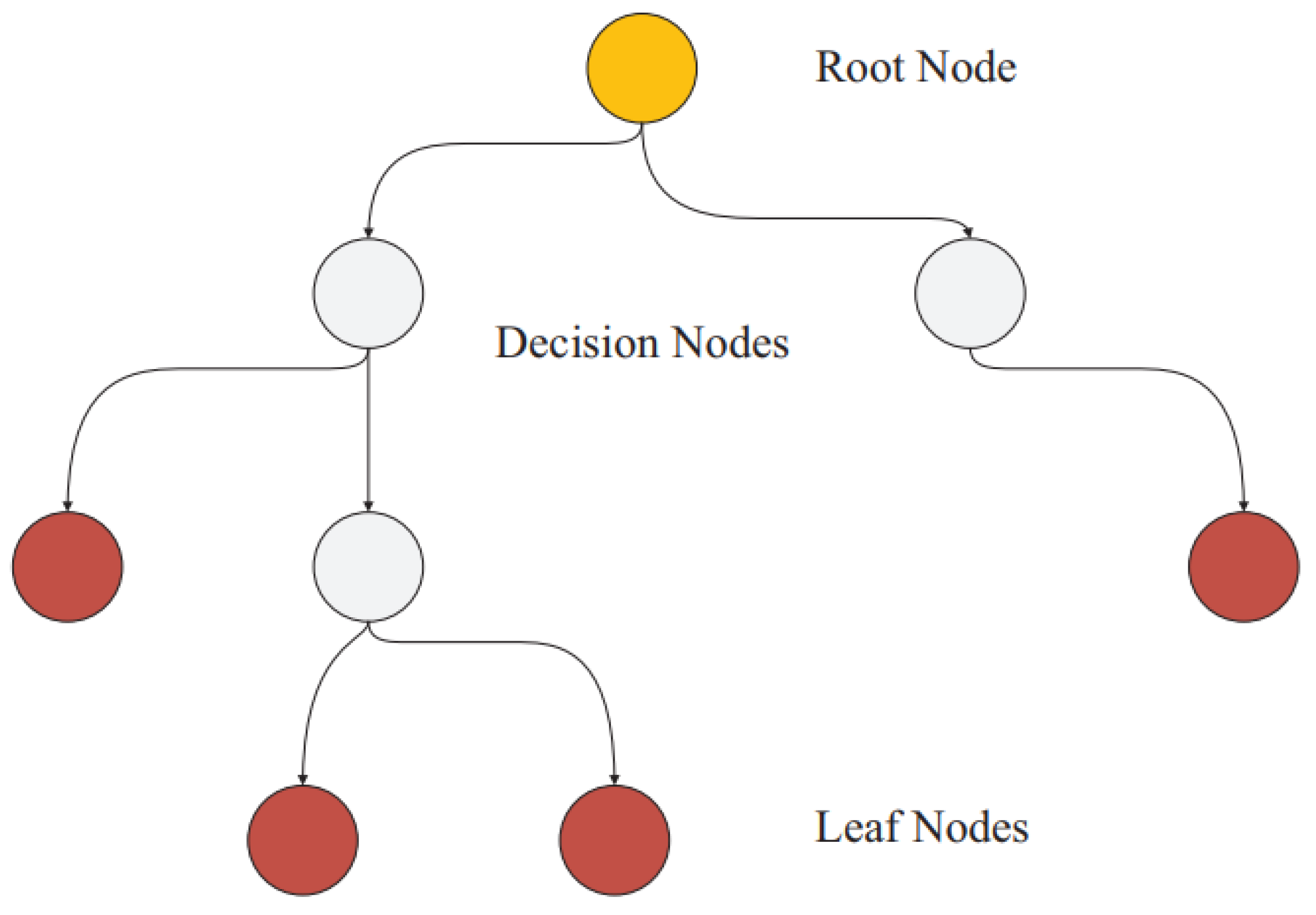
The Regression Decision Trees technique is a critical tool for doing regression prediction. Regression decision trees, also known as regression trees, are an important part of our method for forecasting numerical target variables. These tree-like structures include roots, branches, and leaves, providing a hierarchy that aids with prediction, as showing in Figure 4 [49].

The Regression Decision Trees method in our application starts its prediction trip at the root node, the highest point in the tree. The method runs conditional checks as it proceeds down the tree through internal nodes to discover the best path along the branching structure. Various assessment criteria, such as the total sum of squared errors, lead to this procedure. The algorithm’s prediction conclusion is ultimately formed by the value assigned to the leaf node at the end of the calculated path [49].

The underlying premise of this method in our study is to split and analyze data while attempting to minimize the deviation from the mean of the output characteristics. This partitioning is accomplished by a sequence of splits that divide the data into various subgroups, allowing the algorithm to comprehend underlying patterns and relationships.

The flexibility of Regression Decision Trees to varied settings allows it to capture intricate changes within the data. This approach is a strong tool for regression prediction, particularly when linear or nonlinear correlations between variables are not obvious. By incorporating Regression Decision Trees into our process, we want to take advantage of their ability to find insights and improve the accuracy of our regression predictions.

The process of segregating data into regression trees is conceptually guided by the goal of decreasing the output features’ deviation (D) from the mean [49]. This idea is represented by the equation:

$${\mathrm{D}}_{Total}={\displaystyle \sum }{\left(Y_i-Y\right)}^2$$

(1)

where Y represents the mean of the output features in this context, while Y_i represents the goal feature. As a segmentation point divides the data into two distinct and non-overlapping groups (left and right), the reduction in D may be phrased as follows:

$${\Delta }_{jTotal}={\mathrm{D}}_{Total}-\left({\mathrm{D}}_{Right}+{\mathrm{D}}_{Left}\right)$$

(2)

where D_Right and D_Left represent the differences between the right and left subsets, respectively.

It is critical to stress that several types of regression trees exist, including complicated trees, intermediate trees, and basic trees, which are frequently distinguished by the use of minimal leaf sizes.

6.2. Support Vector Machine

In our pursuit of good regression prediction, the Support Vector Machine (SVM) technique is critical. SVM, a sophisticated machine learning algorithm, is used to model complicated connections between variables and predict numerical goal outcomes. The SVM method uses a structural risk minimization inductive concept at its heart, allowing it to accomplish strong generalization even with a small number of training cases. The calculation of a linear regression function within a higher-dimensional feature space, where input data are processed using nonlinear functions, is the core principle underpinning SVM. This transformation aids in the discovery of complicated linkages that may be hidden within the original data [50].

SVM is specially tailored for regression tasks in our work, where it builds a regression model to predict future outcomes based on observed input data. SVM develops an optimum regression model that aligns with existing knowledge and data patterns by solving a convex quadratic optimization problem. The algorithm’s ability to adapt to tiny sample sizes is very useful, delivering accurate predictions even when data points are scarce. SVM comes in numerous flavors, including linear, quadratic, and cubic SVMs, each with its own set of kernel functions that drive the algorithm’s performance. The kernel function is chosen based on the nature and complexity of the issue, allowing us to customize the method to our unique regression prediction task.

The following equation shows the mathematical kernel function (k) for several models:

$$K\left(x,y\right)={\left[1+\left(\mathrm{x},\mathrm{y}\right)\right]}^P$$

(3)

The parameter P is critical in deciding whether the kernel used in SVM is linear, quadratic, or cubic. SVM may also be divided into fine, medium, and coarse Gaussian classes, with the kernel scale discriminating between them. The kernel scale for the fine class is P/4, the medium scale is P, and the coarse scale is P4, where P denotes the number of predictors.

Although Cortes and Vapnik first proposed the present SVM approach in 1995 [51], SVMs have grown in prominence and are now used by a growing number of researchers [50,52].

6.3. Ensembles

Ensemble approaches, known for their ability to aggregate findings from several separate models, provide a compelling route for improving the predictive capability of the research. Ensemble trees, notably bagged trees and boosted trees, are essential components of the regression prediction process. These strategies tap into the collective wisdom of a large number of decision trees, each of which contributes a unique viewpoint to the overall predictive model [53,54].

The bagged trees, or bootstrap aggregating, method entails building several decision trees from distinct bootstrap samples of the dataset. Individual trees contribute to a final prediction, and the heterogeneity in their outputs is efficiently harnessed to produce a more robust and accurate result. Because the ensemble’s pooled output tends to smooth out the influence of outliers and noise in the data, tagged trees have an inherent capacity to minimize overfitting. Boosted trees, on the other hand, work through an iterative process of improving the performance of each constituent tree. During boosting, the method gives more weight to instances that were incorrectly categorized in prior iterations, prompting the succeeding tree to focus on these difficult situations. This repeated learning process helps the development of a powerful ensemble that constantly refines its predictions, resulting in a more precise and fine-tuned regression model [53,54].

Ensemble trees maximize the individual components’ strengths while limiting their limitations. The ensemble is capable of capturing intricate correlations within the dataset that individual models may miss by pooling the predictions of many trees. As a result, the ensemble tree technique provides this study’s regression prediction models with improved predictive accuracy and generalizability beyond the training data.

The following equation is the mathematical formulation of an ensemble regression tree:

$${\widehat{\mathrm{y}}}_{bag}\left(x\right)=\frac{1}{B}{{\displaystyle \sum }}_{b=1}^B\widehat{\mathrm{Y}}b\left(x\right)$$

(4)

In the equation, $\widehat{\mathrm{y}}$_bag(x) represents the target value obtained through averaging, $\widehat{\mathrm{Y}}$b(x) denotes the predicted target value for observation x in the bth bootstrap sample, and B refers to the total number of bootstrap samples.

6.4. Gaussian Process Regression

GPR emerges as a powerful and adaptable technique for aiding reliable regression predictions. By adopting the ideas of non-parametric modeling and uncertainty quantification, GPR serves as a critical component in our search for exact modeling. GPR is based on the idea of leveraging the flexibility of Gaussian processes to estimate underlying connections in data. Unlike classic regression algorithms, which impose fixed functional forms, GPR takes a more adaptable approach by learning from the data. GPR’s versatility enables it to record complicated and nonlinear patterns that would be difficult to capture using parametric approaches [55]. One of GPR’s distinguishing characteristics is its capacity to measure uncertainty. In our investigation, GPR not only gives predictions but also estimations of related uncertainty. This knowledge is crucial, especially when working with real-world settings with inherent unpredictability and measurement noise. GPR improves the reliability of our regression models by providing a level of confidence in its predictions [56].

GPR works by simulating the connection between input variables and their associated output values using a Gaussian process. A mean function and a covariance function, which represent the central tendency and spatial correlation, respectively, describe this process. GPR iteratively refines its knowledge of the underlying link through Bayesian inference, tailoring its predictions to the available data [56]. Furthermore, GPR provides flexibility with its many kernel functions. We may adjust GPR to the unique properties of our dataset by selecting the appropriate kernel function. Each kernel represents a distinct form of connection, such as smoothness, periodicity, or spatial correlation. This versatility enables GPR to catch different and complicated patterns within data.

GPR modeling is a stochastic approach that simulates random variables using a Gaussian distribution. The Gaussian process is subdivided into squared exponential GPR, Matern GPR, exponential GPR, and rational quadratic GPR. The difference between these specifications is in the kernel function used in each case, as shown below:

• Squared exponential kernel

$$K_{SE}\left(x,\overline{x}\right)={\sigma }^2\exp (-\frac{{\left(x-\overline{x}\right)}^2}{2l^2})$$

(5)

where the parameter “l” determines the characteristic length scale, while σ represents a constant value.

2.

Matern kernel

$$K_m=\frac{1}{2^{\upsilon -1}T\left(\upsilon \right)}(\frac{\sqrt{2\upsilon }}{l}r{)}^{\upsilon }{k}_{\upsilon }(\frac{\sqrt{2\upsilon }}{l}r)$$

(6)

where the value of υ relies on the input distance, and k_υ represents a modified Bessel function. The variables T and r are defined as follows:

$$T=l^{-2}$$

(7)

$$r=\left|\left(x-x^{\prime }\right)\right|$$

(8)

3.

Exponential kernel

$$K_E=\exp ({\left(-\frac{r}{l}\right)}^{\gamma })$$

(9)

where 0 < $\gamma$ ≤ 2.

4.

Rational quadratic kernel

$$K_{RQ}=\left(x,\overline{x}\right)=(1+\frac{{\left(x-\overline{x}\right)}^2}{2\alpha l^2}{)}^{-\alpha }$$

(10)

where α depends on input distance.

6.5. Artificial Neural Network

ANNs function on concepts inspired by the neural architecture of the human brain, mirroring its extensive connectivity and ability to learn from input. A network of linked nodes, or neurons, structured into layers is at the heart of ANNs. An input layer, one or more hidden layers, and an output layer compose these layers. Weighted connections connect each neuron in a layer to neurons in neighboring layers. The intensity and direction of information transmission between neurons are determined by these weights. ANNs are trained by iteratively modifying connection weights to reduce the discrepancy between expected and actual output values. Backpropagation, a process in which the network learns from its faults and adjusts its weights, guides this correction. ANNs successfully learn complicated correlations and patterns in data via this method. Furthermore, ANNs are well-known for their capacity to deal with huge and heterogeneous datasets. Their ability to handle several inputs at the same time and generate continuous output makes them ideal for regression problems. When used for regression prediction, ANNs can uncover hidden insights within the data, resulting in robust and reliable predictions [57].

7. Results and Discussion

In this section, we present a comprehensive analysis of the outcomes derived from employing a diverse range of machine learning techniques, in conjunction with conventional modeling approaches, for the prediction of rutting performance. The assessment of each model’s performance is grounded in a set of carefully chosen performance measures.

$$\mathrm{Mean}\mathrm{Square}\mathrm{Error}\left(\mathrm{MSE}\right)=\frac{1}{n} {{\displaystyle \sum }}_{t=1}^n{\left(\widehat{\mathrm{y}}t-yt\right)}^2$$

(11)

$$\mathrm{Root}\mathrm{Mean}\mathrm{Square}\mathrm{Error}\left(\mathrm{RMSE}\right)=\sqrt{MSE}$$

(12)

$$\mathrm{Mean}\mathrm{Absolute}\mathrm{Error}\left(\mathrm{MAE}\right)=\frac{1}{n} {{\displaystyle \sum }}_{t=1}^n\left|\widehat{\mathrm{y}}t-yt\right|$$

(13)

$$\mathrm{R-Squared}=1-\frac{\mathrm{Sum}\mathrm{of}\mathrm{Squared}\mathrm{Residuals}\left(\mathrm{SSR}\right)}{\mathrm{Total}\mathrm{Sum}\mathrm{of}\mathrm{Squares}\left(\mathrm{TSS}\right)}=1-\frac{{{\displaystyle \sum }}_{t=1}^n{\left(\widehat{\mathrm{y}}t-yt\right)}^2}{{{\displaystyle \sum }}_{t=1}^n{\left(\widehat{\mathrm{y}}-\overline{y}\right)}^2}$$

(14)

In the context of the evaluation, the variables are defined as follows: n represents the number of records, $\widehat{\mathrm{y}}$t stands for the predicted response (i.e., predicted rutting), yt denotes the measured response (i.e., measured rutting), and $\overline{\mathrm{y}}$ represents the average of the measured response.

To mitigate the risk of over-fitting, a 10-fold cross-validation technique was skillfully employed for each model within both scenarios. The results presented herein are based on the means derived from these distinct fivefold runs.

Table 4. Performance measures of machine learning models for all features.

Model Type	Specifications	Performance
		RMSE	R-Squared	MSE	MAE
Linear Regression	Linear	3.19	0.2	10.176	2.3875
	Interactions Linear	10.456	−7.57	109.33	2.4054
	Robust Linear	3.2559	0.17	10.601	2.3559
Regression Tree	Fine	2.6689	0.44	7.1228	1.6955
	Medium	2.739	0.41	7.5019	1.8923
	Coarse	2.8776	0.35	8.2808	2.0683
SVM	Linear SVM	3.2455	0.17	10.534	2.3477
	Quadratic SVM	2.4561	0.53	6.0326	1.6356
	Cubic SVM	2.0819	0.66	4.3345	1.3801
	Fine Gaussian	2.6802	0.44	7.1837	1.8364
	Medium Gaussian	2.4096	0.55	5.8059	1.5915
	Coarse Gaussian	3.2155	0.19	10.339	2.3016
Ensemble Trees	Boosted trees	2.5647	0.48	6.5778	1.842
	Bagged trees	2.1877	0.62	4.7862	1.5312
GPR	Squared Exponential GPR	1.9911	0.69	3.9644	1.3358
	Matern 5/2 GPR	1.9675	0.7	3.8709	1.3235
	Exponential GPR	1.9963	0.69	3.9854	1.3753
	Rational Quadratic GPR	1.9665	0.7	3.8672	1.3229
ANN	Narrow Neural Network (10 neurons)	2.4565	0.53	6.0342	1.7425
	Medium Neural Network (25 neurons)	2.5288	0.5	6.3946	1.8247
	Wide Neural Network (100 neurons)	2.8329	0.37	8.0256	2.0242
	Bilayered Neural Network	2.4994	0.51	6.2472	1.788
	Trilayered Neural Network	2.5631	0.49	6.5697	1.8057

and

Table 5. Performance measures of machine learning models for selected features.

Model Type	Specifications	Performance
		RMSE	R-Squared	MSE	MAE
Linear Regression	Linear	3.2437	0.18	10.521	2.3978
	Interactions Linear	2.7551	0.41	7.5904	1.9876
	Robust Linear	3.2923	0.15	10.839	2.3672
Regression Tree	Fine	2.5792	0.48	6.6522	1.7201
	Medium	2.6986	0.43	7.2825	1.8919
	Coarse	2.9407	0.32	8.6475	2.1482
SVM	Linear	3.2805	0.16	10.762	2.368
	Quadratic	2.7665	0.4	7.6537	1.8928
	Cubic	2.2246	0.61	4.9487	1.5045
	Fine Gaussian	2.5289	0.5	6.3956	1.7386
	Medium Gaussian	2.5314	0.5	6.4082	1.7114
	Coarse Gaussian	3.2437	0.18	10.521	2.3138
Ensembles Trees	Boosted Trees	2.5942	0.47	6.7299	1.8877
	Bagged Trees	2.2673	0.6	5.1404	1.5968
GPR	Squared Exponential	1.9613	0.7	3.8467	1.3511
	Matern 5/2 GPR	1.9412	0.7	3.7681	1.3355
	Exponential GPR	1.9903	0.69	3.9612	1.3914
	Rational Quadratic	1.9371	0.71	3.7522	1.3308
ANN	Narrow(10 neurons)	2.7287	0.42	7.446	1.9862
	Medium (25 neurons)	2.4406	0.53	5.9568	1.7653
	Wide (100 neurons)	2.787	0.39	7.7673	2.0023
	Bilayered	2.5171	0.5	6.3357	1.8043
	Trilayered	2.6783	0.44	7.1731	1.9049

present the results of machine learning models’ performance, categorized by the utilization of all selected features and a subset of selected features, providing valuable insights into the predictive capabilities of each model. The comprehensive analysis of machine learning models’ performance under different feature scenarios, encompassing all selected features and a subset thereof, provides valuable insights into their predictive capabilities for rutting behavior in pavement engineering.

Examining the results for all selected features, it is evident that Linear Regression models, including Linear, Interactions Linear, and Robust Linear, exhibit limited predictive power, as indicated by their relatively high Root Mean Squared Error (RMSE) values (e.g., Linear: 3.19) and modest R-Squared values (e.g., Linear: 0.2). This suggests that linear relationships between features and the response variable may not adequately capture the complexities inherent in rutting behavior. In contrast, the performance of Regression Trees improves with finer granularity (e.g., Fine: RMSE = 2.6689, R-Squared = 0.44), underlining the significance of feature interactions in accurate prediction.

Among the Support Vector Machine (SVM) models, the Cubic SVM stands out with notably high R-Squared (e.g., 0.66) and low RMSE (e.g., 2.0819) values. This highlights the potential of SVM models with higher-order polynomial kernels to capture intricate relationships in the data. Gaussian Process Regression (GPR) models consistently display superior predictive accuracy, with Rational Quadratic GPR yielding an RMSE of 1.9665 and R-Squared of 0.7, further affirming their suitability for rutting prediction.

Ensemble Trees, represented by Boosted Trees (e.g., RMSE = 2.5647, R-Squared = 0.48) and Bagged Trees (e.g., RMSE = 2.1877, R-Squared = 0.62), continue to demonstrate competitive performance. The ensemble approach harnesses the strengths of multiple models, leading to improved predictive accuracy.

Shifting focus to a selected subset of features, intriguing trends emerge. Linear Regression models, including Interactions Linear and Robust Linear, exhibit notable improvements in predictive performance, with reduced RMSE values and enhanced R-Squared values. This suggests that a carefully curated subset of features aligns better with the linear assumptions of these models.

Regression Trees maintain their favorable performance trends in the selected feature scenario, underlining their capability to capture complex feature interactions (e.g., Fine: RMSE = 2.5792, R-Squared = 0.48). SVM models, especially Quadratic and Cubic SVM, display mixed enhancements (e.g., Cubic SVM: RMSE = 2.2246, R-Squared = 0.61), showcasing the impact of feature selection on higher-order relationships.

GPR models maintain impressive predictive accuracy across selected features (e.g., Rational Quadratic GPR: RMSE = 1.9371, R-Squared = 0.71), further establishing their suitability for rutting prediction.

Ensemble Trees, particularly Boosted Trees (e.g., RMSE = 2.5942, R-Squared = 0.47) and Bagged Trees (e.g., RMSE = 2.2673, R-Squared = 0.6), continue to exhibit competitive performance in the selected feature scenario, reinforcing their robustness. Several studies in the literature have similarly highlighted the effectiveness of these advanced techniques in enhancing pavement performance prediction models [58,59,60,61].

It is noteworthy that few instances within our modeling process yielded negative R-Squared values. This phenomenon arises when the model’s predictive performance falls considerably short in comparison to the baseline prediction achieved by using the mean value of the dependent variable. This scenario is a result of the Sum of Squares Residual (SSR), which quantifies the variability unaccounted for by the model, exceeding the Total Sum of Squares (TSSs), which encapsulates the overall variability in the data. When the SSR/TSS ratio surpasses 1.0, as is the case with negative R-Squared values, it indicates that the model’s inability to explain the variance outweighs even the basic approach of using the mean. This situation prompts a thorough examination of model assumptions, data quality, and feature relevance. While negative R-Squared values may initially raise concerns, they ultimately serve as a valuable diagnostic tool, directing us to refine and enhance our modeling strategy to achieve more meaningful insights from the data [62].

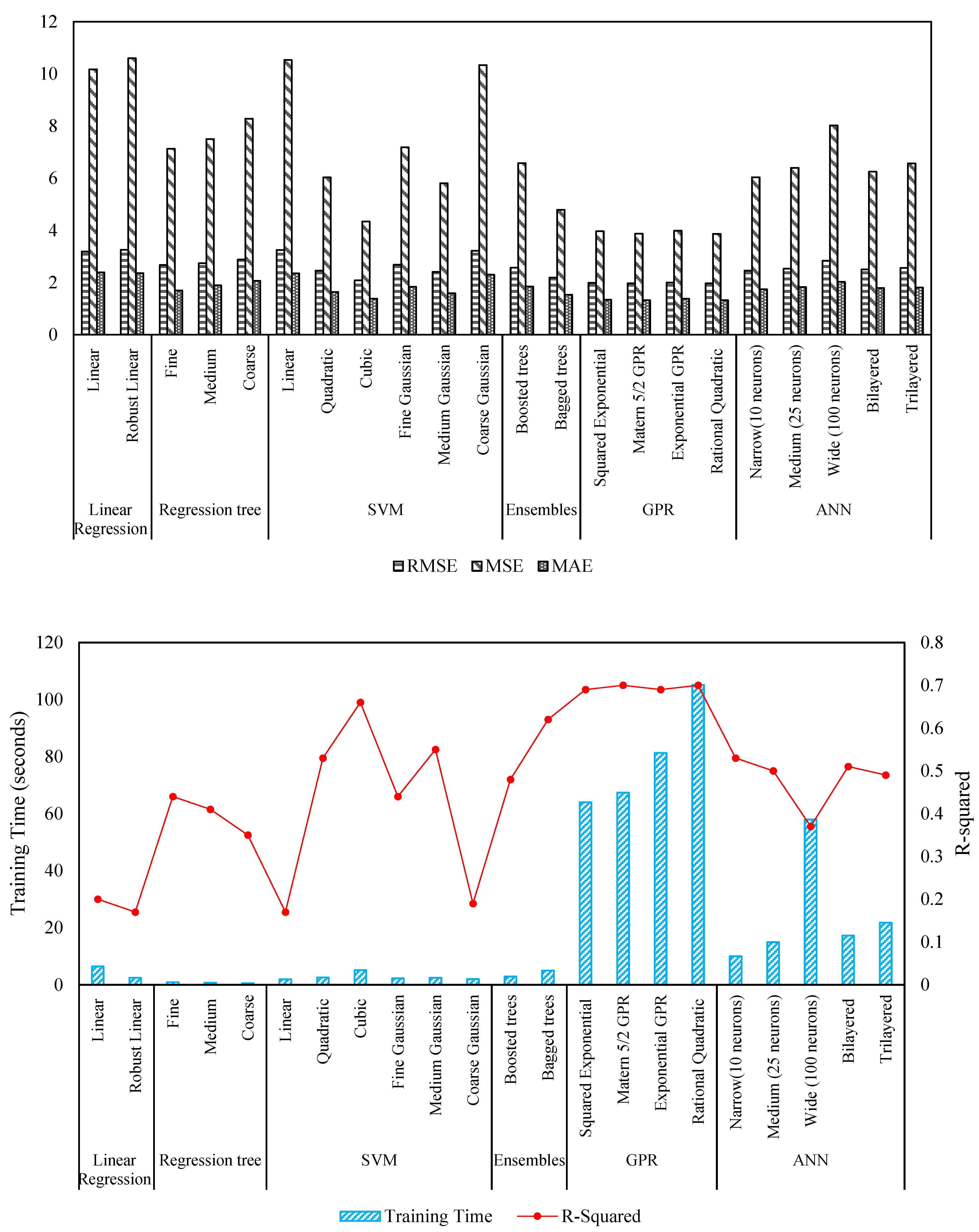
Figure 5 and Figure 6 serve as graphical representations summarizing the performance measures across all machine learning models, considering both scenarios, encompassing the utilization of all features and the selective incorporation of features.

The training times for various machine learning models, coupled with their corresponding accuracy levels, provide a deeper understanding of the trade-offs between computational efficiency and predictive performance.

When using all available features, some models showcase remarkable efficiency in terms of training times. Notably, the Regression Tree models, including Fine, Medium, and Coarse granularity, exhibit relatively short training times while delivering competitive accuracy. These models strike a balance between computation and prediction, making them appealing choices for applications where real-time processing is essential.

Linear models, such as Linear Regression and Robust Linear Regression, also stand out for their quick training times. Although their accuracy may not match the complexity of certain other models, their efficiency can make them suitable for time-sensitive scenarios.

However, it is important to note that certain high-performing models come at the cost of longer training times. Gaussian Process Regression (GPR) models, particularly Squared Exponential and Matern 5/2, demonstrate extended training times while delivering strong accuracy. The Rational Quadratic GPR model, with its superior accuracy, also falls into this category. These longer training times can be attributed to the intricate relationships GPR captures within the data.

Transitioning to selected features offers insights into the interplay between feature reduction, training times, and accuracy. Linear Regression models with selected features show reduced training times, maintaining a reasonable compromise between computational efficiency and accuracy. The Interactions Linear Regression model, despite a slight increase in training time, retains competitive accuracy levels, showcasing the benefits of feature selection.

Ensemble methods, like Boosted Trees and Bagged Trees, maintain consistent training times across both feature scenarios. Their accuracy levels are notably robust to feature reduction, making them stable choices when optimizing for both efficiency and performance.

Gaussian Process Regression models persist as time-intensive options, irrespective of feature selection. These models continue to provide high accuracy while demanding more training time, emphasizing the intricate nature of their predictions.

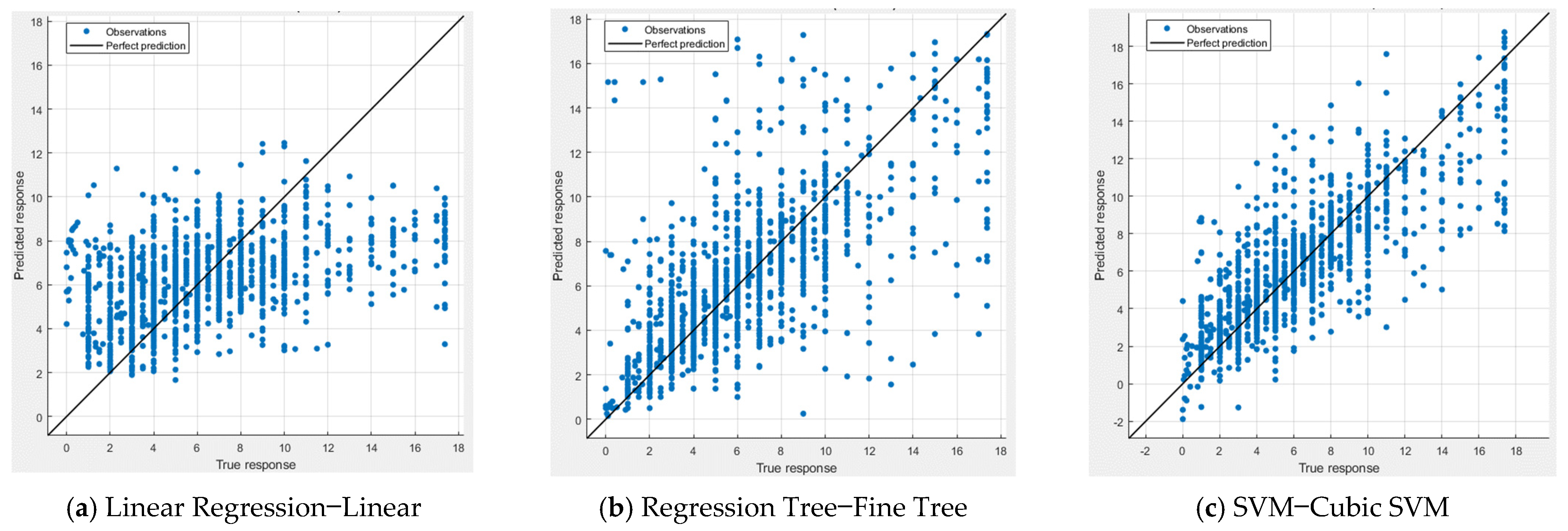
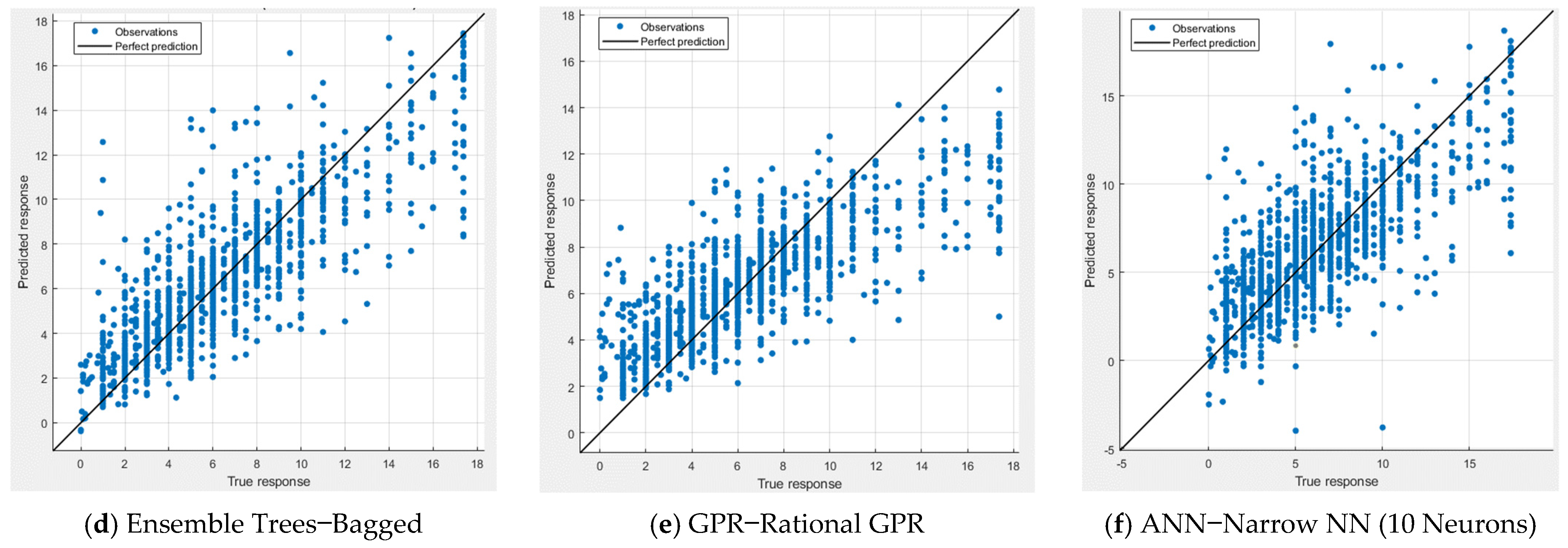
Figure 7 and Figure 8 display the performance measures of the top models developed using each modeling technique for both the cases of using all features and using only selected features. In both figures, the comparison between the measured and predicted rutting values is presented. The models generally exhibit a pattern with most points aligned along the equality line, suggesting a good fit. However, a few records appear to deviate from this line. The Exponential GPR model stands out as the best scatter diagram, supporting the earlier findings and conclusions.

8. Comparison Analysis

8.1. Model Selection

In the pursuit of robust rut depth prediction models for flexible pavements, this study draws inspiration from two notable prior works that have tackled similar challenges. The first model, presented by Radwan et al. (2020), focuses primarily on hot climate regions, recognizing the heightened significance of rutting in such conditions [63]. In their work, they proposed empirical models for rut depth prediction tailored to wet no-freeze and dry no-freeze zones. The models take into account several key variables, emphasizing the influence of environmental and traffic-related factors.

For the wet no-freeze zone, Radwan et al. (2020) formulated the rut depth model as follows [63]:

RutDepth = 10.097 − 0.987 ln(ESAL) + 0.478 Va

(15)

In the dry no-freeze zone, their model is represented as:

RutDepth = 21.39 + 0.009 ESAL − 1.05 Ta + 0.255 Va

(16)

Here, ESAL denotes the Equivalent Single Axle Load, Va is the Air Voids in the Asphalt Layer, and Ta represents the annual average temperature.

In contrast, Naiel (2010) introduced a rut depth model applicable to different climate zones. For the wet no-freeze zone, their model is presented as [64]:

Ln(RutDepth) = 0.9 + 0.19 (AC%) − 0.077(SN) + 0.063 Ln (KESAL)

(17)

For the dry no-freeze zone, the model is expressed as:

Ln(RutDepth) = 0.681 + 0.114 Ln(KESAL) + 0.007 (D > 32 °C)

(18)

here AC % signifies the percentage of asphalt content, SN denotes the structural number, KESAL represents the equivalent single axle load, and D is the temperature in degrees Celsius.

In the present study, we endeavored to build upon the insights provided by Radwan et al. (2020) [63] and Naiel (2010) [64] by leveraging the extensive Long-Term Pavement Performance (LTPP) database. Our methodology encompasses data retrieval from the LTPP database, data preprocessing, and the application of advanced machine-learning techniques. The resultant predictive models aim to offer an improved understanding of rut depth patterns in various climate zones and provide valuable tools for pavement management systems.

Comparing our models to those of Radwan et al. (2020) [63] and Naiel (2010) [64], several distinctions emerge. Firstly, our approach adopts a data-driven, machine learning-based methodology, which inherently differs from the empirical modeling employed in the prior studies. This allows for a more flexible and adaptable modeling framework capable of capturing complex interactions between attributes.

Secondly, our models incorporate a broader set of attributes, drawn from the LTPP database, encompassing not only climatic and traffic-related factors but also structural and material properties. This holistic approach seeks to enhance the accuracy and robustness of rut depth predictions.

8.2. Comparison and Analysis

To assess the effectiveness of our novel machine learning-driven models in predicting rut depth compared with existing empirical models, we conducted a rigorous comparison analysis using real-world data from different states located in wet non-freeze and dry non-freeze (hot climate regions).

Table 6. Data collected for model comparison.

State	Section No.	Climate Region	SN	AC %	No. Lanes	Layer 2 Thickness (mm)	Layer 3 Thickness (mm)	Layer 4 Thickness (mm)	Annual Average Precip (mm)	Annual Average Temp (°C)	Freeze Index	Annual Average Humidity	AADTT	KESAL	Va
Alabama	01-4125	Wet, No-Freeze	4.1	4.7	2	165	165	86	1581.4	17	4	70.5	674	196	5.818
Arizona	04-C340	Dry, No-Freeze	4.2	5	3	284	175	15	141.2	19.9	0	53.5	300	150	Assumed 7
Arkansas	05-3048	Wet, No-Freeze	4.2	4.5	1	188	74	48	1592.2	17	28	64	126	56	3.535
California	06-8201	Wet, No-Freeze	4	6.2	1	178	122	114	392.7	15.6	0	60.5	125	21	8.144
Florida	12-9054	Wet, No-Freeze	3.9	Assumed 5	2	305	251	64	1480.9	20.4	0	63.5	425	173	3.993
Missouri	29-0501	Wet, No-Freeze	4.3	4.9	1	102	185	28	1031.9	14.5	84	65	595	195	6.95
New Mexico	35-1112	Dry, No-Freeze	3.7	5	2	163	137	20	650.3	17	15	57	139	51	6.639
New Mexico	35-6401	Dry, No-Freeze	5.8	5.8	2	152	150	102	350.7	10.7	158	57	3614	507	3.592
Oklahoma	40-4165	Wet, No-Freeze	4	5	1	140	69	0	917.1	15.3	81	65.5	349	113	5.263
South Carolina	45-1008	Wet, No-Freeze	2.4	6.2	1	198	56	38	1587.5	13.8	10	67.5	62	7	3.214

summarizes the data collected for model comparison, including various attributes ranging from climatic conditions to structural properties.

We then compared the predictions made by Radwan et al. (2020) [63], Naiel (2010) [64], and our newly developed machine learning models with the measured rut depths for these sections. The results are summarized in

Table 7. Comparison of predicted and measured rut depths.

State	Section No.	Measured Values	Radwan et al. (2020) [63]	Naiel (2010) [64]	Our New Model
Alabama	812667	10.00	7.62	6.11	9.49
Arizona	04-C340	18.00	3.63	4.38	16.49
Arkansas	419421	6.00	7.79	5.39	6.32
California	2301546	4.00	7.28	7.11	4.23
Florida	2613281	17.00	6.89	2.52	14.98
Missouri	29-0501	10.50	8.16	6.25	10.42
New Mexico	35-1112	5.00	9.32	3.87	5.46
New Mexico	35-6401	4.00	5.97	5.03	5.17
Oklahoma	40-4165	6.00	7.90	6.30	7.34
South Carolina	45-1008	6.00	9.69	7.51	6.23

.

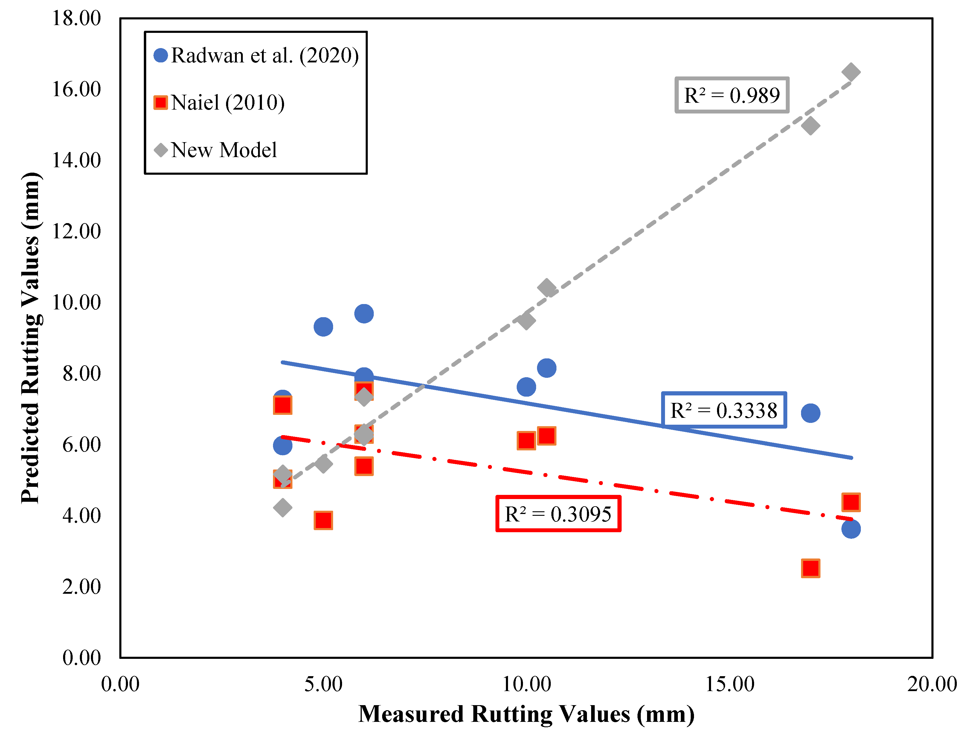
The comparison results indicate that our new machine-learning model consistently outperforms Radwan et al. (2020) [63] and Naiel (2010) [64] in predicting rut depth across different states and climate zones. Notably, the coefficient of determination (R²) for our model is significantly higher, with an R² of 0.989, indicating a strong correlation between predicted and measured rut depths as shown in Figure 9. In contrast, the R² values for Radwan et al. (2020) [63] and Naiel (2010) [64] are 0.303 and 0.3095, respectively.

These findings underscore the superior predictive capabilities of our machine learning-driven approach in capturing the complexities of rut depth formation and development, especially in the context of varying climate conditions and pavement attributes. This enhanced accuracy can be a valuable asset for pavement management systems, enabling more informed decision-making and cost-effective maintenance strategies.

9. Conclusions

This study primarily centered on the development of rutting models through the implementation of various machine learning techniques, utilizing data extracted from the Long-Term Pavement Performance (LTPP) database. The analysis and results of the study led to the following conclusions:

• By examining correlating plots, the aim was to uncover clear patterns that could help us predict rutting in asphalt pavements. However, it was observed that there were no distinct and readily identifiable patterns between the dependent variable (rutting) and the other independent design factors.
• Using the analytical capabilities of the Weka Software, a thorough investigation of the most linked features in relation to the dependent variable (rutting) was conducted. Interestingly, this analysis discovered that the final portion of the features had a negative average merit value. As a result, a judicious approach was taken, which resulted in the first 22 features being chosen as the most relevant in the predictive modeling process.
• A notable trend emerged, portraying the superior predictive prowess of models employing Regression Trees (RT), Gaussian Process Regression (GPR), Support Vector Machines (SVM), Ensemble Trees (ET), and Artificial Neural Networks (ANN). These models consistently exhibited higher performance accuracy in comparison to linear regression methods, accentuating the potential of advanced machine learning techniques in pavement performance prediction.
• For all features, the best-performing model is Rational Quadratic GPR yielding RMSE of 1.9665, R-Squared of 0.7, MSE of 3.8672, and MAE of 1.3229, while the worst-performing model, Interactions Linear, with RMSE of 10.456, R-Squared of 7.57 MSE 109.33 and MAE of 2.4054.
• For selected features, the best-performing model is Rational Quadratic GPR with RMSE of 1.9371, R-Squared of 0.71, MSE of 3.7522, and MAE of 1.3308, while the worst-performing model was Robust Linear, producing RMSE of 3.2923, R-Squared of 0.15 MSE of 10.839 and MAE of 2.3672.
• It can be noticed that for all features and selected features scenarios, both have the same best-performing model which is Rational Quadratic GPR with similar performance values. This highlights GPR’s potential as a powerful tool for rutting prediction in pavement engineering.
• The analysis highlights the substantial impact of feature selection on the predictive accuracy of various machine learning models. Specifically, the utilization of a selected subset of features consistently leads to improved model performance, showcasing the significance of careful feature curation.
• Ensemble trees, represented by Boosted Trees and Bagged Trees, consistently display competitive performance across both feature scenarios. This robustness underscores the effectiveness of ensemble techniques in capturing complex relationships and improving prediction accuracy.
• The insights derived from this comprehensive analysis can guide the selection of appropriate machine learning models and feature subsets for rutting prediction. This offers valuable decision support for pavement engineers and researchers seeking to enhance the accuracy of pavement performance models.
• Our novel machine learning model outperforms existing models, with an R² of 0.989 compared with 0.303 and 0.3095 for other models. This demonstrates the potential of advanced machine learning in accurate rut depth prediction across diverse climates, aiding pavement management decisions.”

10. Limitations and Future Work

While our study presents valuable insights into rutting prediction using machine learning techniques and the Long-Term Pavement Performance (LTPP) database, certain limitations deserve consideration. Firstly, the available dataset might encompass inherent biases or limitations that could influence the generalizability of our findings. Additionally, the predictive accuracy of our models may be influenced by the quality and representativeness of the LTPP data, potentially affecting the applicability of our results to broader road infrastructure contexts. Furthermore, our study primarily focuses on the attributes available within the LTPP database, which may not capture all relevant variables that could impact rutting, thus warranting caution in extrapolating the findings to factors beyond the dataset’s scope.

Looking ahead, there are several promising directions for extending and enhancing our research. Exploring hybrid models that combine machine learning techniques with domain-specific knowledge or physical models can yield more interpretable and accurate predictions. Temporal analysis can offer insights into rutting trends and variations over time, contributing to the development of predictive models that account for dynamic road conditions. Furthermore, the integration of data from diverse sources or additional road databases can provide a more comprehensive understanding of rutting dynamics and further refine our predictive models. As road infrastructure continues to evolve, our study encourages the exploration of these avenues to ensure the continued relevance and applicability of rutting prediction models in practical engineering scenarios.