1. Introduction
The integration of urban city energy management systems has become increasingly important for the optimization of urban services such as energy, transportation, and public safety [
1]. These systems use advanced technologies like sensors, data analytics, and AI to collect and process data in real-time, allowing city managers to make data-driven decisions that improve the efficiency and sustainability of urban services [
2]. One area where urban city energy management systems can make a significant impact is in the optimization of energy usage, reduction of carbon footprint, and improvement of overall energy efficiency [
3]. Wind energy is a renewable energy source that can contribute to these goals, but its intermittent and variable nature can create instability in the power grid [
4].
Renewable wind energy plays a vital role in meeting global energy demands, with the Global Wind Energy Council reporting a total capacity of 743 GW by the end of 2020. Growth projections indicate an average yearly increase of 12.7% over the next five years, leading to an estimated total capacity of 1.4 TW by the end of 2026. The need for wind energy stems from the critical need to address greenhouse gas emissions and tackle climate change. Wind energy, being a sustainable and eco-friendly power source, has the potential to diminish reliance on fossil fuels, contributing to the pursuit of carbon neutrality. Additionally, wind energy can improve energy security and promote sustainable development. The increasing demand for wind energy is driven by supportive government policies, decreasing costs of wind power generation, and growing public awareness of environmental issues. Wind energy forecasting refers to predicting the overall energy that can be harnessed from wind sources over a certain period, often encompassing multiple wind turbines or a wind farm. On the other hand, wind power forecasting narrows down the focus to predicting the actual electrical power output from individual wind turbines or a wind farm. In this article, the active power has been predicted using the historical data from the wind turbine dataset.
The wind power generated by the wind turbine’s rotor (
) is expressed as follows:
where
denotes the density of the air in kg/m
3, R indicates the rotor radius in meters, v denotes the wind speed in meter/second,
is the rotor power coefficient, which is a function of the pitch angle
and tip speed ratio
. As indicated in Equation (1), factors such as air density (
), rotor radius (R), wind speed (v), and other parameters influence the power output of a wind turbine. These factors play a critical role in determining the efficiency of wind energy conversion.
Alongside the constant parameters, wind speed emerges as a pivotal variable that directly impacts the power output of a wind turbine. The dataset includes wind speed as one of the features in our wind power forecasting model. Moreover, we have taken into consideration an additional nine parameters to formulate the wind power prediction, and this is explained in the subsequent sections.
Wind energy forecasting plays a crucial role in enhancing the operation of urban city energy management systems. It enables the anticipation of changes in wind power output, facilitating grid adjustments to ensure stability and reliability [
5]. This forecasting is particularly valuable for short-term wind power prediction, empowering grid operators to proactively respond to variations in wind power output to maintain grid stability [
6]. Accurate wind power forecasting also empowers energy providers to optimize their resource management, minimizing the reliance on costly backup power sources. Furthermore, it facilitates real-time energy trading in electricity markets, contributing to a cleaner and more sustainable energy future while reducing dependence on traditional energy sources [
7].
Deep learning techniques have proven to be exceptionally proficient in wind power forecasting to reveal intricate patterns and correlations within extensive and intricate datasets, a challenge that conventional methods may find difficult to address [
8]. Wind power prediction plays a vital role in various timeframes, encompassing very short-term intervals (few minutes to half an hour) for activities like regulation, real-time grid operations, turbine control, and market clearing. Similarly, short-term periods (ranging from 30 min to 6 h) are employed for load dispatch planning and making well-informed choices regarding load management. Medium-term durations (ranging from 6 h to 1 day) play a critical role in ensuring the stability of electricity markets, facilitating energy trading, and making well-informed decisions regarding online and offline generating capacity. On the other hand, long-term periods (spanning from 1 day to a month) are utilized for determining reserve requirements, establishing maintenance schedules, optimizing operational costs, and efficiently managing power system operations.
The motivation driving this research is rooted in the urgent need to transition towards sustainable energy practices to counter the escalating challenges posed by climate change and depleting fossil fuel reserves. The imperative to reduce greenhouse gas emissions and enhance energy efficiency has led to a growing emphasis on harnessing renewable energy sources like wind power. However, the inherent variability of wind energy necessitates advanced forecasting models to enable its efficient integration into urban energy systems. The research is further motivated by the potential to revolutionize urban energy management, reduce reliance on non-renewable sources, and pave the way for a cleaner and more sustainable energy future.
The significance of this research is two-fold. Firstly, the accurate wind power forecasting model empowers urban energy managers to optimize energy consumption patterns, reducing costs and the carbon footprint. Secondly, by promoting wind energy integration into urban energy management, this research aligns with renewable energy goals and sustainable development, contributing to greener and more resilient cities.
In this article, a short-term wind power forecasting model has been proposed using LSTM neural networks based on historical data. By accurately forecasting wind power, urban city energy management systems can better manage their energy resources, reduce their carbon footprint, and promote a cleaner and more sustainable energy future.
Literature Review
Chen, Q. and Folly, K.A. [
9] developed a short-term wind power forecasting model to optimize power systems with significant wind power integration. To achieve this, they introduced a novel approach called “mixed input features-based cascade-connected artificial neural network” (ANN). This approach aimed to improve forecasting accuracy by incorporating input features from neighboring stations while effectively addressing overfitting issues. As a result, their proposed method showed promising results in enhancing the performance of ANNs.
Li, Z. et al. [
10] presented an approach for short-term wind power forecasting, which combines Extreme Learning Machines (ELM) with error correction models. This innovative approach resulted in remarkable advancements in the accuracy of ultra-short-term forecasting.
Kramer, O. and Gieseke, F. [
11] conducted a study exploring the potential of Support Vector Regression (SVR) in wind energy prediction using data from the NREL western wind resource dataset and the available windmill infrastructure. The research focused on parameterizing the loss function of SVR and aimed to establish the reliability of wind forecasts at both micro and macro levels. The performance of the SVR-based wind energy forecast was evaluated for individual wind grid points and entire wind parks, while also determining the optimal amount of historical data required for precise prediction.
Y. Kassa et al. [
12] introduced an adaptive neuro-fuzzy inference system (ANFIS) technique for forecasting one-day-ahead hourly wind power generation. Given the intermittent and unpredictable nature of wind energy, precise wind power forecasting is crucial to ensure a dependable power supply. The proposed ANFIS approach exhibited superior performance compared to BP neural network-based and hybrid GA-BP NN-based models in terms of both accuracy and reliability. The evaluation was conducted using practical data from a wind turbine in a microgrid located in Beijing.
Tu, C.-S. et al. [
13] introduced a model for short-term wind power forecasting that relies on historical marine weather and wind power data. To enhance computing efficiency, they divided the dataset into clusters using a data regression algorithm. The team constructed a regression model based on the principles of the least squares support vector machine (LSSVM) and further optimized LSSVM parameters using enhanced bee swarm optimization. The study emphasized the challenges posed by the intermittent and uncertain nature of wind power, highlighting the importance of accurate wind power forecasting for efficient power system operation and reliability. When compared to other tested models, the proposed method demonstrated superior performance and showed potential for large-scale wind power grid integration.
Pang, M. et al. [
14] proposed an innovative wind speed forecasting model that utilizes a broad learning system (BLS). This model employed enhanced variational mode decomposition (EVMD) and subseries reconstruction (SR) techniques, surpassing traditional methods. By adaptively dividing subseries based on sample entropy and characterizing their complexity as high or low entropy, wind speed forecasts for the reconstructed subseries were generated using the EVMD-SR-BLS-ARIMA hybrid wind speed prediction model.
Najeebullah et al. [
15] focuses on machine-learning (ML)-based short-term wind power prediction using a hybrid model. The dataset includes real-time wind speed, humidity, temperature, and wind power values from 2007 to 2011. The ML model employs SVR, Meta-Heuristic Neural Networks (MHNN), and Enhanced Particle Swarm Optimization (EPSO). They achieved a standard deviation of error of 0.0766 for the test set.
Alkesaiberi et al. [
16] focuses on efficient wind power prediction using machine learning methods. Three datasets from different sources are used: France, Turkey, and Kaggle. Wind turbine data, including variables like wind speed and direction, are analyzed. Static and dynamic models are tested, with dynamic models utilizing past data information performing better. Including meteorological variables enhances prediction accuracy. Kernel-driven models (SVR, GPR) and ensemble learning models (Boosting, Bagging, XGBoost, RF) are compared. Results show that dynamic GPR and ensemble models provide satisfactory predictions, with an R
2 of around 0.95 on average.
Table 1 provides the various wind power prediction models and methods employed.
Most of the reported works use limited input features to develop the prediction model and claim higher performance. In this article, a short-term wind power forecasting model has been proposed using LSTM neural networks based on historical data. By accurately forecasting wind power, urban city energy management systems can better manage their energy resources, reduce their carbon footprint, and promote a cleaner and more sustainable energy future. Our research pays particular attention to the data pre-processing phase, where we emphasize the removal of outliers. By strategically removing outliers from the dataset, our LSTM model achieves a higher level of stability and accuracy. This approach results in a more reliable and trustworthy wind power forecasting model compared to methods that may not account for outlier removal comprehensively.
The major contributions of the article are
- ✓
The article leverages state-of-the-art technologies such as LSTM neural networks, which have demonstrated remarkable proficiency in handling complex patterns and correlations within extensive datasets. LSTM’s ability to capture long-term dependencies makes it particularly suitable for accurate wind power forecasting.
- ✓
To enhance the accuracy of the model, the article employs the Pearson correlation technique for feature selection. This approach ensures that only crucial features are considered, resulting in improved forecasting performance.
- ✓
The article implements effective data pre-processing techniques, including outlier removal, to guarantee that the LSTM model is trained on a representative dataset. By removing outliers, the model achieves a higher level of stability and accuracy. Also, the article offers insightful observations regarding daily and monthly trends in wind energy generation and related features.
- ✓
The article underscores the practical application of the proposed model in urban city energy management systems. Precise wind power prediction plays a critical role in optimizing energy consumption, reducing the carbon footprint, and promoting a cleaner and more sustainable energy future.
- ✓
The integration of wind power forecasting into urban city energy management systems can significantly contribute to addressing greenhouse gas emissions and climate change. The model’s accurate predictions facilitate the efficient utilization of wind energy, leading to reduced reliance on fossil fuels and fostering sustainable development.
2. Materials and Methods
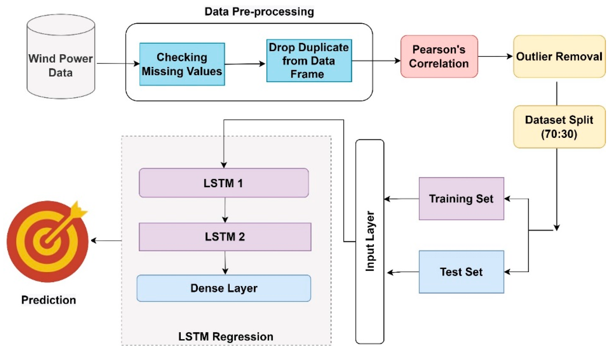
The proposed methodology block diagram is presented in
Figure 1, which consists of several stages, including data pre-processing, Pearson correlation, outlier removal, LSTM model development, and performance evaluation. The subsequent sections elaborate on each stage and describe how the model was developed.
2.1. Data
The wind energy system dataset is adopted from a public database [
22] and it contains 118,224 instances and 22 attributes. The dataset used for analysis includes recordings taken at 10 min intervals from January 2018 to March 2020, making it suitable for short-term forecasting purposes. The first attribute is “Date”, which is of object type and contains the date of each observation. The rest of the features contain numerical data of float64 type, except for two object type columns: “WTG”, which stands for wind turbine generator and “TurbineStatus”. As shown in
Table 2, each attribute represents various measurements related to wind turbine operation, including ambient temperature, blade pitch angle, gearbox oil temperature, wind direction, and wind speed. While some attributes might not have an immediately apparent relationship to wind power prediction, it is important to consider that wind turbine operation is influenced by a range of environmental and operational factors.
Attributes like “Bearing Shaft Temperature”, “Gearbox Bearing Temperature”, “Gearbox Oil Temperature”, and “Generator Winding Temperature” might not directly represent wind speed or active power, but they can provide valuable insights into the operational conditions of the wind turbine. Changes in these temperatures could be indicative of factors such as mechanical stress, friction, and wear. While higher wind speeds might contribute to increased temperatures in certain turbine components due to enhanced mechanical activity, it is essential to recognize that multiple interacting factors contribute to these temperature variations. Moreover, the thermal behavior of these components can also affect their efficiency and overall performance. To validate the impact of these attributes on short term wind power forecasting, Pearson correlation was utilized to identify attributes that exhibit significant correlations with the target variable, i.e., Active Power.
Some of the columns have missing values, indicated by “Non-Null Count” being less than the total number of entries in the dataset. The missing values may need to be handled before analyzing the data.
2.2. Data Pre-Processing
Deep learning models rely on having comprehensive data to effectively capture the patterns and dependencies among features and the target variable. Missing values can lead to incomplete data, which may result in a biased or inaccurate model [
23]. Missing values can also affect the performance of some evaluation metrics such as mean squared error (MSE) or mean absolute error (MAE), which are commonly used to evaluate the performance of regression models [
24]. Therefore, it is decided to remove missing or null values from the dataset before training a deep learning model to avoid these issues. After removing the missing and null values, the dataset has 32,728 instances.
2.3. Pearson Correlation
When developing a deep learning-based regression model, it is essential to select relevant features. The Pearson correlation coefficient [
25] between the target variable and each feature can be calculated to identify the highly correlated features that can be used in the regression model, thus improving its accuracy and performance. The Pearson’s correlation coefficient (
r) can be expressed as shown in Equation (2).
where,
= the Pearson correlation coefficient for the variables
x and
y;
n = the total number of observations;
= p’s value (for ith observation);
= q’s value (for ith observation).
2.4. Outlier Removal
Outliers can arise from errors in data collection, measurement inaccuracies, or other anomalies within the data. Outlier removal is the process of identifying and removing these data points from the dataset [
26].
Outlier removal is an important step in deep-learning-based model development because outliers can have a significant influence on the model performance. Outliers can lead to incorrect model training, inaccurate predictions, and reduced model accuracy. By removing outliers, the model can be trained on a more representative dataset and can lead to improved model performance. Additionally, removing outliers can reduce the variability in the data, leading to a more stable model.
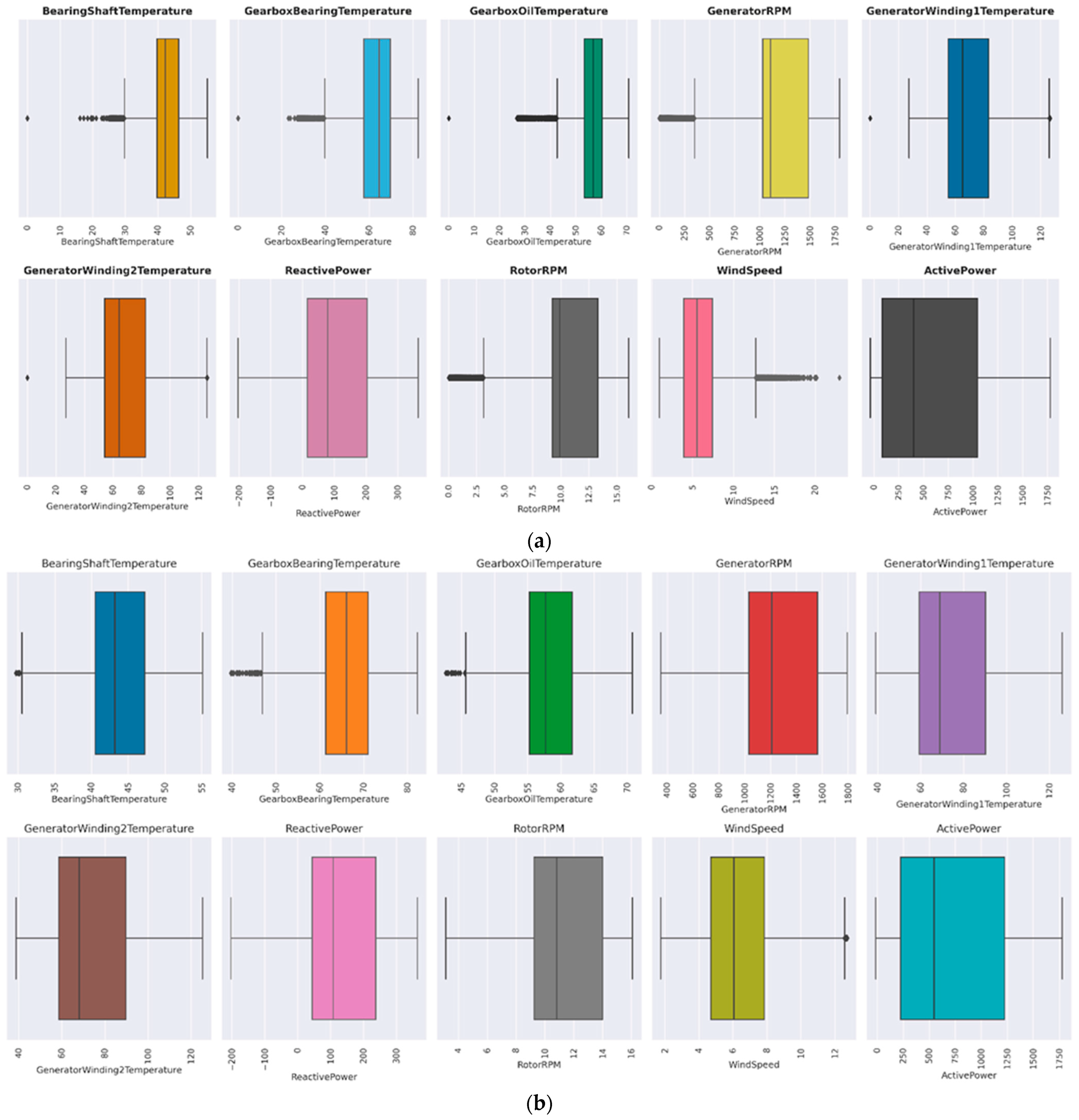
Figure 2a,b shows the Box Plot of before outlier removal and after outlier removal of the dataset.
The interquartile range (IQR) of each feature has been calculated, which is the range between the first and third quartile of the data. Equations (3) and (4) are used to calculate the lower and upper bounds for each column:
Equation (3) calculates the lower bound for outlier removal. Q1 represents the first quartile, which is the value below which 25% of the data fall. By subtracting 1.5 times the IQR from Q1, we define a threshold below which data points are considered outliers.
Equation (4) calculates the upper bound for outlier removal. Q3 represents the third quartile, which is the value below which 75% of the data fall. By adding 1.5 times the IQR to Q3, we define a threshold above which data points are considered outliers.
These thresholds, calculated based on the quartiles and the interquartile range, help identify and remove outliers from the dataset, ensuring that the deep learning model is trained on a representative and accurate dataset. Removing outliers contributes to a more stable and accurate model, as it reduces the impact of erroneous data points on the training process and the final predictions.
2.5. Data Analysis
After the removal of outliers, the total number of instances reduces to 27,310. LSTM models are particularly sensitive to the distribution and patterns within the data. Outliers can disrupt the underlying temporal dependencies and patterns that LSTM models excel at capturing. Eliminating outliers allows the LSTM model to focus on learning meaningful temporal relationships within the data without being influenced by extreme values that might not repeat in the future.
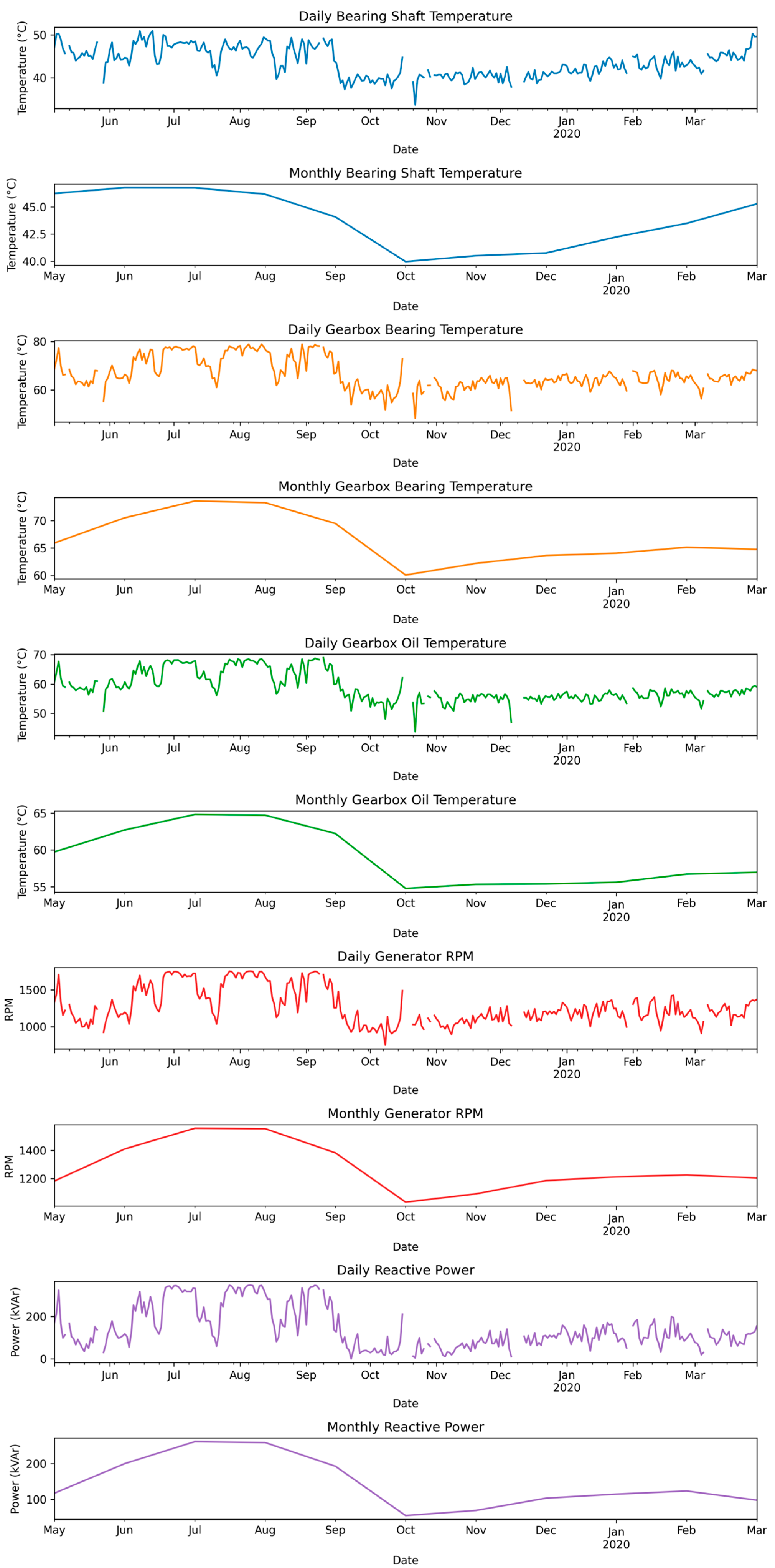
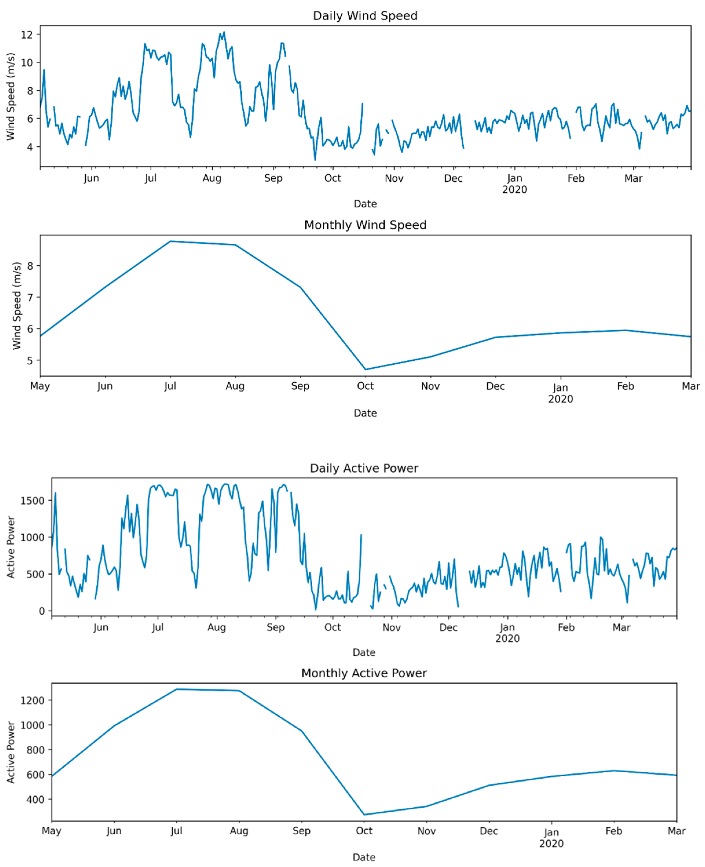
Figure 3 provides valuable insights into the daily and monthly trends of all features. The bearing shaft temperature exhibits a peak from May to mid-September, followed by a decline in October. This temperature pattern can be attributed to higher ambient temperatures and increased solar radiation during the summer months. These factors can contribute to elevated temperatures in various wind turbine components, including the bearing shaft. Elevated temperatures can lead to increased friction and heat generation within the bearings, resulting in higher temperatures. As the weather cools down in October, ambient temperatures decrease, leading to a reduction in bearing temperatures. This trend is consistent with most other features, as highly correlated attributes were considered during the model’s development.
Furthermore, wind power generation experiences its highest output during July and August, followed by a notable drop in October. Weather systems, such as high-pressure areas and temperature gradients, play a role in influencing wind speeds. During the summer, specific weather patterns can lead to increased wind speeds. These enhanced wind speeds subsequently improve wind turbine efficiency, contributing to higher power generation. The analysis of mean monthly data reveals the long-term dependency of other aspects of electrical power generation, while mean daily active power output data captures daily fluctuations, providing crucial short-term dependency information.
In the plot representing the period from May to September, which corresponds to the annual peak power generation, there is a dip in wind speed and related features observed in mid-July and August, as evident from the daily mean plot. Wind turbines are designed to operate optimally within specific wind speed ranges. The consistent wind speeds during July and August falling within this optimal range can enable turbines to harness more wind energy, resulting in higher power output.
These insights provide a deeper understanding of the intricate interplay of various factors influencing power generation trends. This understanding can be pivotal in optimizing energy management strategies and addressing fluctuations in power generation, ultimately contributing to more efficient and sustainable energy practices.
2.6. LSTM Model Development
The LSTM model has been employed for wind power prediction using time series data.
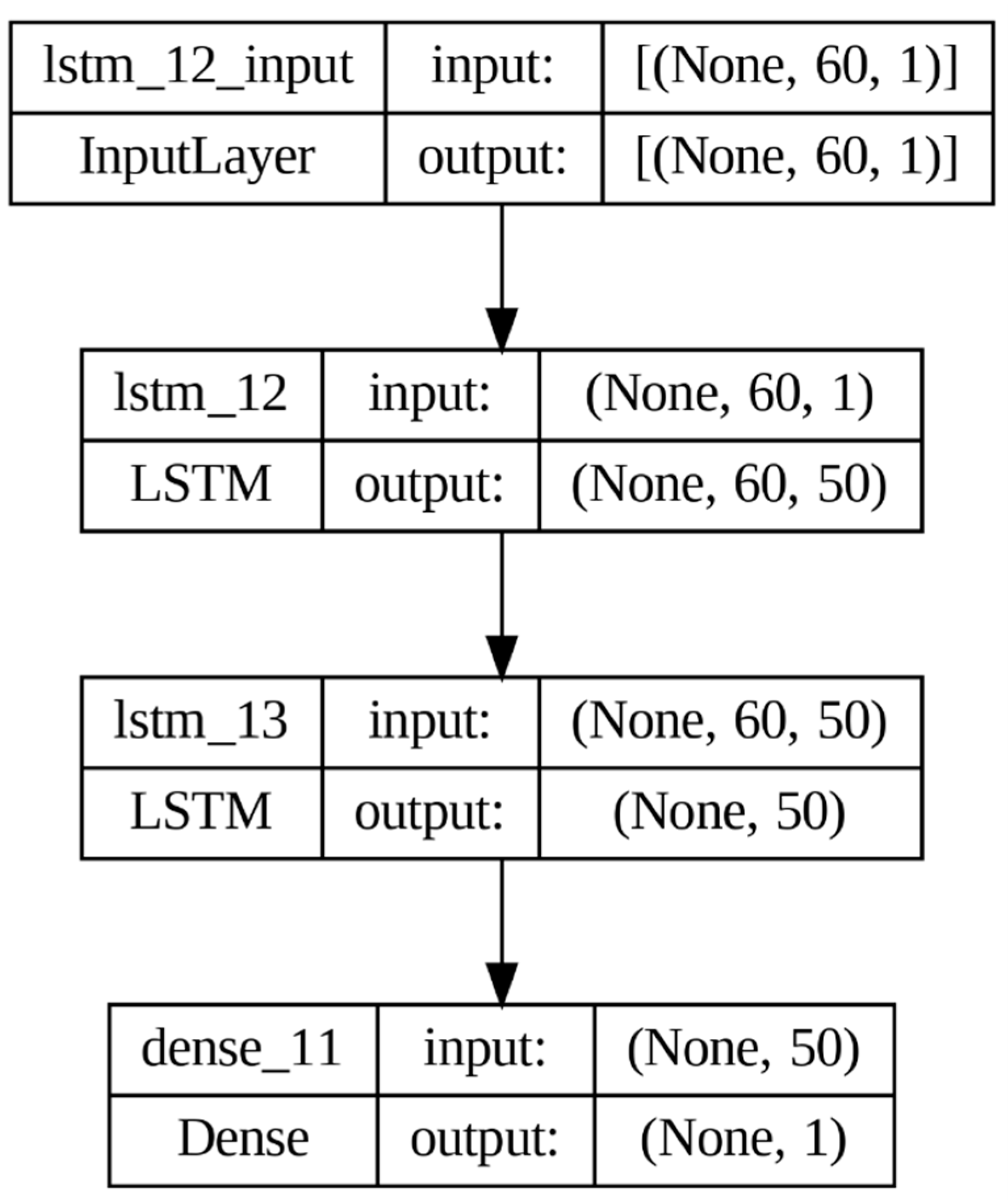
Figure 4 displays the proposed LSTM model. Initially, the data are pre-processed by extracting the target variable, normalizing it, and splitting it into training and testing sets with 70:30 ratio, respectively. The time step is defined as 60, and the training and testing data are created accordingly.
The LSTM model architecture [
27] is constructed using Keras’ sequential model, which includes two LSTM layers, each with 50 units, along with a dense output layer. The model is built using the Adam optimizer and utilizes the MSE loss function.
The model performance has been assessed using various metrics like MAE, MSE, and root mean squared error. By leveraging this approach, real-time wind power generation prediction becomes possible, assisting energy companies in optimizing their operations and reducing costs.
Equations (5)–(10) show in concise form the forward pass of an LSTM cell with a forget gate. The lowercase variables represent vectors. These equations define the LSTM model’s complex mechanism for controlling information flow, which makes it suitable for handling long-term dependencies in sequential data [
28].
Equation (5) calculates the forget gate. is the sigmoid activation function, and are the input and previous hidden state weights, and is the bias term. Equation (6) computes the input gate to update the cell state. is input gate output, and it determines how much of the should be added to the cell state. Equation (7) calculates the output gate. is the output of the output gate. Equation (8) computes the new candidate cell state . Equation (9) computes the new cell state by compounding the output of the forget gate and the new candidate cell state . Equation (10) computes the new hidden state by applying the output gate to the cell state and passing it through a tanh activation function. The output is then multiplied element-wise with the output gate .
2.7. Performance Metrics
The evaluation of the regression model’s effectiveness was conducted through metrics [
29] including MAE, MSE, Root Mean Squared Error (RMSE), and the R-squared value. The calculation of MAE is based on Equation (11).
The MSE is determined using Equation (12).
The RMSE is determined using Equation (13).
Here, and are the actual and predicted values for “n” number of instances.
R-Squared (R
2) or coefficient of determination is calculated by Equation (14).
Here, is mean of all the actual values.
3. Results and Discussion
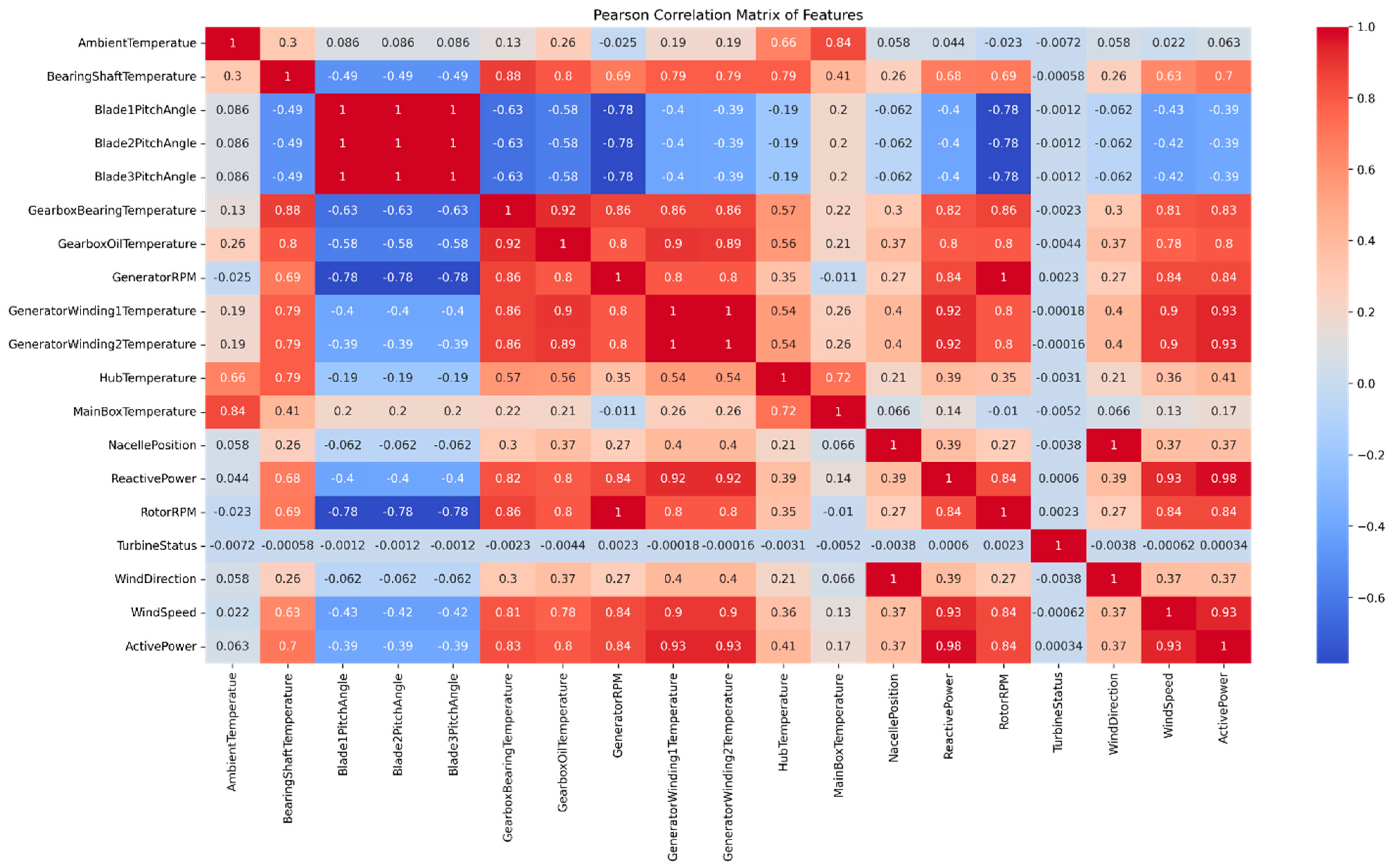
The Pearson correlation matrix for the preprocessed dataset has been shown in
Figure 5. The results show the Pearson correlation matrix of all the features and the features that have a correlation coefficient greater than 0.5 has been selected with the target variable. These features are considered important as they have a strong relationship with the target variable and are likely to have a significant impact on the prediction accuracy of the model. In this case, the selected features are “BearingShaftTemperature”, “GearboxBearingTemperature”, “GearboxOilTemperature”, “GeneratorRPM”, “GeneratorWinding1Temperature”, “GeneratorWinding2Temperature”, “ReactivePower”, “RotorRPM”, “WindSpeed”, “ActivePower”. These 10 features can be used as input variables for the deep learning model. Here, the Active Power will be the target variable.
The trained LSTM regression model encapsulates the learned patterns and correlations from the historical wind energy data. In this research work, the dataset was initially divided into a 70:30 ratio for training and testing. Out of the total 27,310 instances remaining after the outlier removal process, 19,117 instances were used for training, and 8193 instances were allocated for the test set. These test inputs will have the same attributes (features) that were used during training, such as wind speed, temperature, generator RPM, etc. Next, feed the test data into the loaded LSTM model. The model’s forward pass involves passing the input data through the layers, applying the learned weights and biases, and generating predictions. Once the model generates predictions, the resulting active power value will be compared with the actual active power value present in the test set.
The LSTM regression model was assessed with the test dataset, employing several performance metrics including MAE, MSE, RMSE, and R
2.
Figure 6 illustrates the plot of the loss function during training.
To monitor the training process, the model is trained for 50 epochs with a batch size of 32, and the loss curve is plotted. Following training, the model is utilized to make predictions on the test data, and the obtained results are compared to the actual data using visual plots.
The model achieved an MAE of 107.132, MSE of 22,910.49, RMSE of 151.36, and an R
2 score of 0.9108 in the test data.
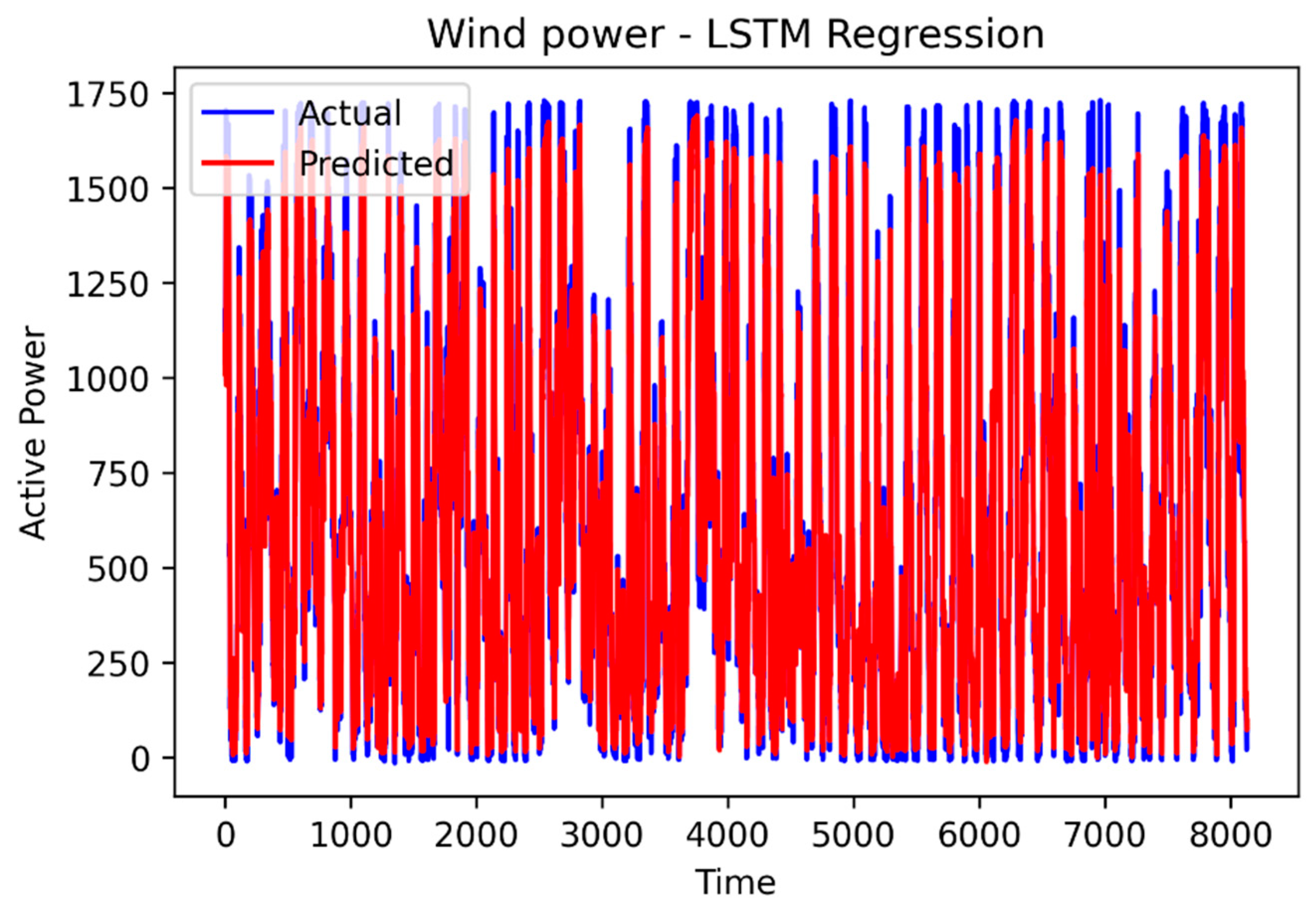
Figure 7 illustrates the output of the LSTM regression model on the test set, showing a close alignment between the predicted and actual values of wind power, indicating the model’s effectiveness.
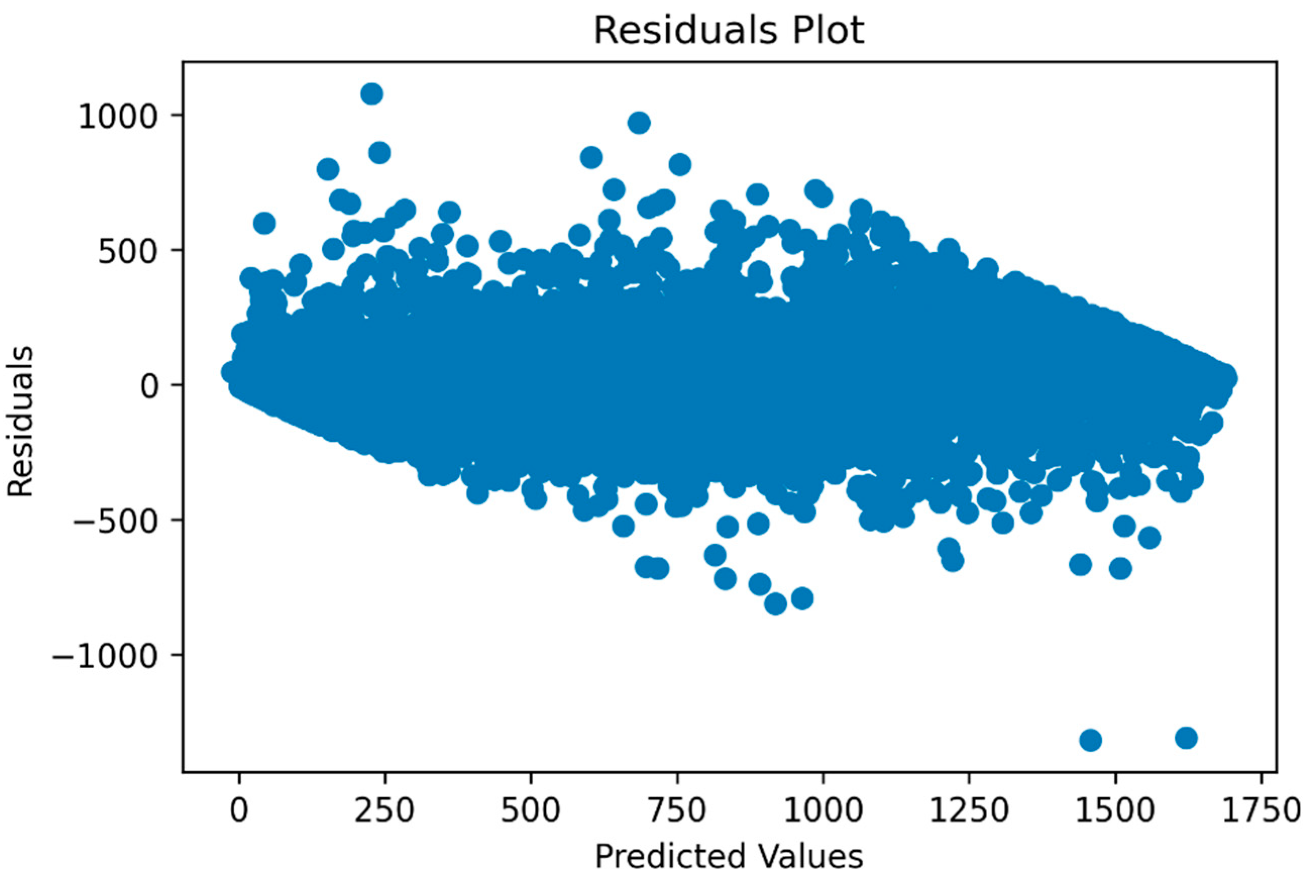
Figure 8 displays the residual plot, demonstrating that the residuals are randomly scattered around the horizontal line, indicating the absence of systematic errors or heteroscedasticity in the model. Additionally,
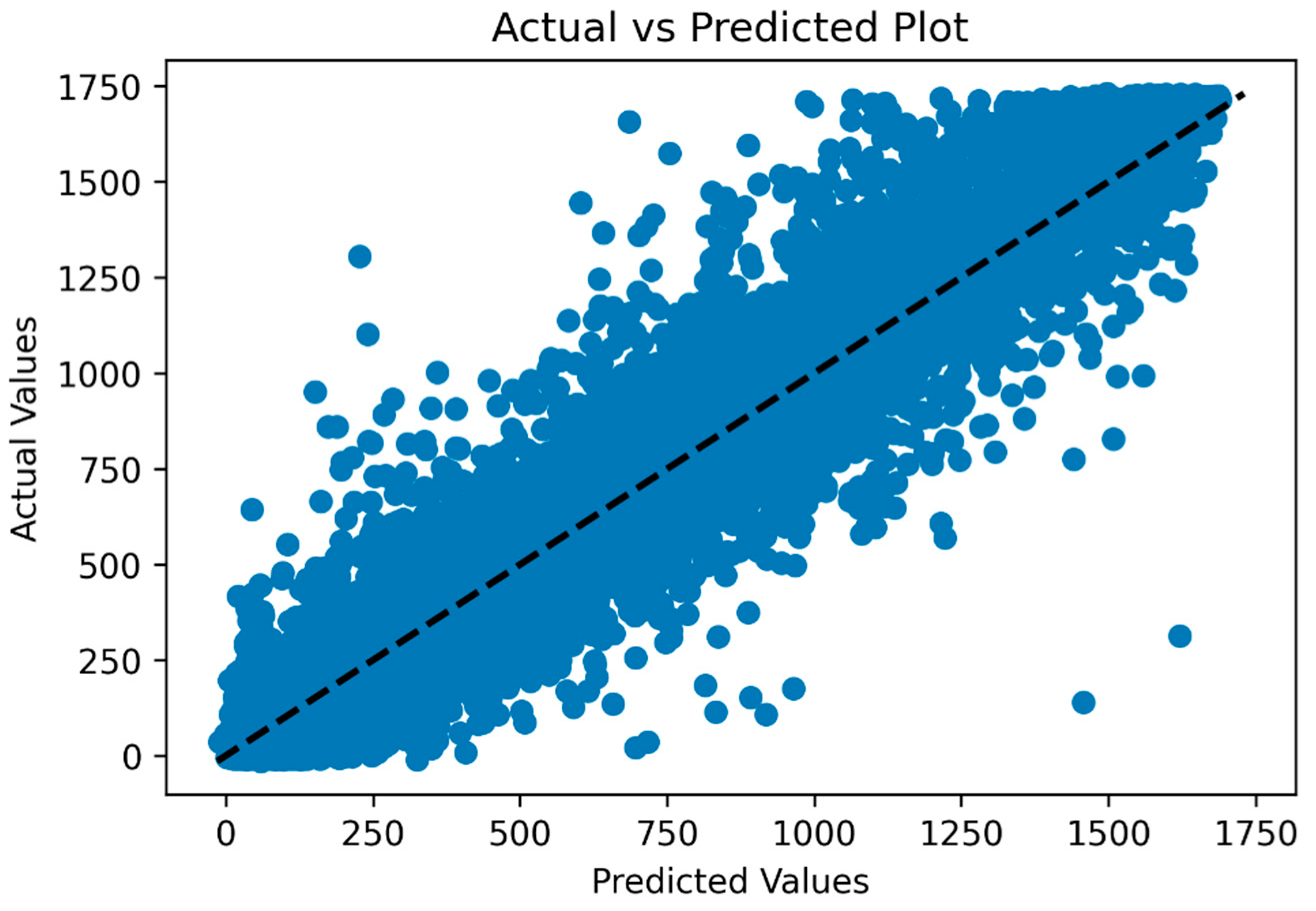
Figure 9 depicts the plot of actual versus predicted wind power generation values, showcasing a strong linear relationship between the two, affirming the model’s accuracy in prediction. The dotted line provides a visual reference for how well the model’s predictions align with the actual data.
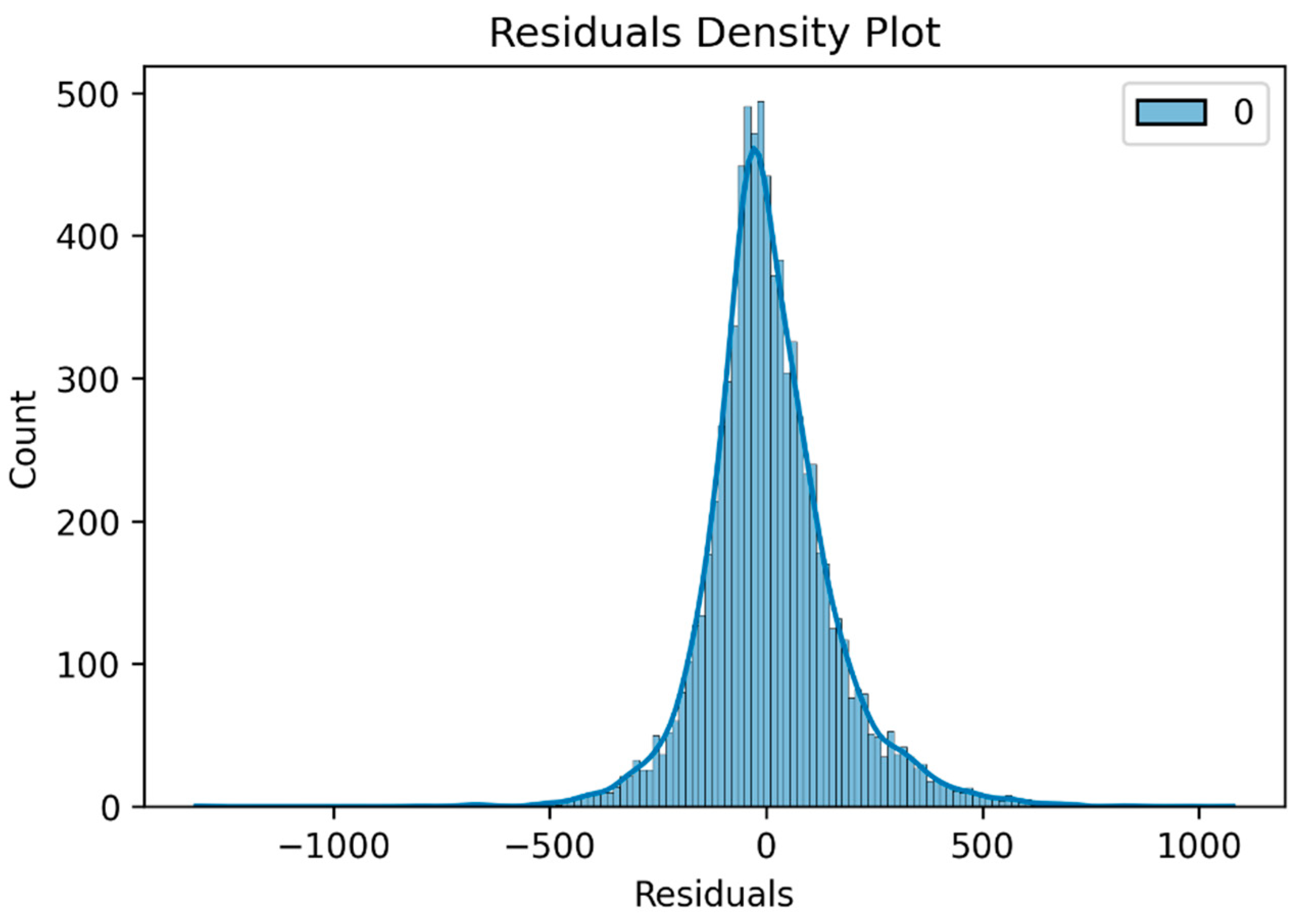
Figure 10 presents the residual density plot, indicating that the residuals are approximately normally distributed, reflecting the model’s well-calibrated nature in accurately predicting wind power generation.
The LSTM regression model developed in this study has proven its capability to accurately predict wind power generation based on historical data. The high accuracy and ability to explain a substantial proportion of variance in the test data make it a valuable tool for city managers to optimize energy consumption and minimize waste. For instance, the model’s predictions can help identify periods of high energy consumption, enabling proactive measures to reduce grid load. Moreover, the model’s capability to forecast energy demand for different timeframes allows for the efficient utilization of renewable energy sources and a reduction in non-renewable sources.
The results suggest that the LSTM regression model can be an instrumental asset in the development of renewable energy systems and energy grid planning, contributing to more efficient and sustainable energy management practices.
Table 3 provides a comprehensive comparison of the performance of the proposed LSTM-based wind power forecasting approach with existing research studies that employed different models. The Mean Absolute Error (MAE) and Root Mean Squared Error (RMSE) are used as evaluation metrics to assess the accuracy of the forecasting models. The models from Ryu et al. [
30] encompass different variants of ARIMA and other regression techniques. Notably, our proposed LSTM approach consistently outperforms all models from Ryu et al. in terms of both MAE and RMSE. This underscores the superiority of the LSTM model in capturing complex patterns and dependencies within wind power data. Comparing our results with those of Mora et al. [
31], who explored different LSTM architectures, reveals that our LSTM approach achieves substantially lower MAE and RMSE values. This outcome reinforces the efficacy of our approach in wind power forecasting. The lower MAE and RMSE values achieved by our proposed approach demonstrate its high accuracy and predictive capabilities. By leveraging LSTM’s ability to capture long-term dependencies and its feature selection techniques, our model achieves superior performance in comparison to previous studies.
4. Conclusions
Integrating wind power forecasting into urban city energy management systems is significant for optimizing energy usage, reducing the carbon footprint, and improving overall energy efficiency. The proposed LSTM-based model for short-term wind power forecasting, which was developed and evaluated using a publicly available dataset, achieved a MAE of 107.132, MSE of 22,910.49, RMSE of 151.36, and an R2 score of 0.9108 for the test set. The results of this study can be utilized by city managers to optimize energy consumption and reduce waste, as well as to forecast energy demand for different times of the day or year. It has been found that the LSTM regression model can be valuable in the development of renewable energy systems and the planning of energy grids.
Looking towards the future, there are several exciting directions for further exploration and enhancement. Continual advancements in deep learning techniques, such as novel LSTM architectures or hybrid models, could potentially yield even higher predictive accuracy and efficiency. Furthermore, integrating real-time data sources and leveraging advancements in data assimilation techniques can lead to dynamic and adaptive wind power forecasting systems that react swiftly to changing conditions. Expanding the scope of forecasting models to encompass other renewable sources, such as solar energy, and effectively combining their predictions could offer a comprehensive view of urban energy availability.
