Data Preprocessing and Machine Learning Modeling for Rockburst Assessment

Abstract

Rockbursts pose a significant threat to human safety and environmental stability. This paper aims to predict rockburst intensity using a machine learning model. A dataset containing 344 rockburst cases was collected, with eight inducing features as input and four rockburst grades as output. In the preprocessing stage, missing feature values were estimated using a regression imputation strategy. A novel approach, which combines feature selection (FS), t-distributed stochastic neighbor embedding (t-SNE), and Gaussian mixture model (GMM) clustering, was proposed to relabel the dataset. The effectiveness of this approach was compared with common statistical methods, and its underlying principles were analyzed. A voting ensemble strategy was used to build the machine learning model, and optimal hyperparameters were determined using the tree-structured Parzen estimator (TPE), whose efficiency and accuracy were compared with three common optimization algorithms. The best combination model was determined using performance evaluation and subsequently applied to practical rockburst prediction. Finally, feature sensitivity was studied using a relative importance analysis. The results indicate that the FS + t-SNE + GMM approach stands out as the optimum data preprocessing method, significantly improving the prediction accuracy and generalization ability of the model. TPE is the most effective optimization algorithm, characterized simultaneously by both high search capability and efficiency. Moreover, the elastic energy index W_et, the maximum circumferential stress of surrounding rock σ_θ, and the uniaxial compression strength of rock σ_c were identified as relatively important features in the rockburst prediction model.

1. Introduction

Tunnels excavated in tectonically active areas or deep underground spaces are susceptible to rockbursts, which can lead to numerous casualties or property losses [1]. For instance, in the Witwatersrand mines of South Africa, rockbursts resulted in 435 deaths [2]. Similarly, in Jinping II Hydropower Station, China, seven deaths were reported and one tunnel boring machine was damaged in a rockburst catastrophe [3]. Additionally, rockbursts can trigger serious environmental problems. The fragmentation and collapse of surrounding rock can damage stratum integrity and stability. Moreover, new water passage may form in the broken rock layer, altering groundwater flow and impacting ecosystem stability [4,5]. Consequently, predicting rockbursts is of utmost importance to mitigate these adverse consequences, enhance environmental management efficiency, and promote sustainable development.

The prediction of rockbursts involves two main aspects. One aspect focuses on short-term risk forecasting, which includes capturing precursory information and providing early warnings based on field monitoring. Various advanced monitoring methods are widely used in underground fields, such as electromagnetic radiation [6], acoustic emission [7], microseismic monitoring [8], vibration [9], and electrical resistance [10]. Short-term risk prediction plays a critical role in minimizing damage during the construction stage, as it relies on processing physical information released by the surrounding rock before a rockburst occurs. However, this approach might not distinctly identify the specific features that induce rockbursts. On the other hand, long-term risk estimation serves as another aspect of rockburst prediction, addressing the limitations of short-term risk prediction. Studies in this field have been conducted using three methods: empirical proneness indices, numerical simulations, and machine learning models. Several proneness indices have found practical application in engineering, including the Turchaninov criterion [11], E.Hoek criterion [12], energy storage index W_et [13], bursting energy index K_E [14], residual elastic energy index [15], and strength brittleness coefficient σ_c/c_t [16]. Despite the efforts invested in the development of these indices, they often address only specific aspects of rockbursts and are formulated based on particular engineering cases, limiting their applicability to diverse geological conditions. To enhance the accuracy of rockburst prediction for specific scenarios, numerical models coupled with rockburst assessment indices have been designed to pinpoint the occurrence locations and ranges of rockbursts [17,18,19,20,21]. Nevertheless, constructing intricate models and determining material parameters that accurately reflect real-world engineering conditions can be time-consuming and may not readily extend to different cases. Moreover, the selection of assessment indices directly impacts the prediction outcomes, but a reliable criterion for their selection is lacking. The rapid advancement of artificial intelligence (AI) has opened opportunities to solve various engineering challenges using data-driven approaches [22,23]. AI’s capability to unveil nonlinear relationships presents a promising avenue for underground construction [24,25]. In summary, traditional proneness indices often provide a moderate level of predictive accuracy due to their reliance on engineering experience. Numerical methods exhibit limited generalization due to the incorporation of assumptions that may not precisely mirror real-world engineering conditions, which poses challenges for their application in diverse projects. In contrast, machine learning holds promise as an approach to explore the connection between inducing features and rockburst intensity without prior assumptions [26], and its applicability is readily evident.

Data preprocessing constitutes the initial stage of machine learning, where the quality of the dataset significantly influences the effectiveness of training machine learning models. In practice, data related to rockbursts collected from in situ measurements may encounter challenges such as data imbalance, partial missing values, and inconsistent labeling criteria. To address the issues posed by unbalanced data, Yin et al. [27,28] utilized techniques such as principal component analysis (PCA), the synthetic minority over-sampling technique (SMOTE), and ensemble models to mitigate the adverse effects. Xue et al. [29] combined Copula theory and Monte Carlo simulation to oversample data with relatively small sample sizes in their labels. Regarding missing values in some features, Li et al. [30] used the expectation maximization (EM) algorithm to input missing values. As for label-related problems, some unsupervised learning methods were utilized to relabel original data, such as the K-means method, elbow method, and others [31]. These data preprocessing methods mentioned above can enhance the performance of machine learning models to a certain extent by adjusting the dataset from a statistical perspective. However, they might lack consideration for the physical meaning and interrelationships between features, potentially leading to differences from the real data.

The second step involves constructing machine learning models using specific algorithms. In the field of rockbursts, researchers have attempted to investigate the complex relationship between geological conditions and rockburst grades using a variety of machine learning models. For instance, Zhou et al. [32] used eleven common algorithms to evaluate their ability to learn rockbursts. Faradonbeh et al. [33] introduced two robust algorithms (gene expression programming and decision tree) to predict rockburst risk indices, effectively addressing the “black-box” property often associated with many machine learning algorithms. Guo et al. [34] extended the application of multivariate adaptive regression splines and deep forest algorithms to classify rockburst intensity, deriving explicit mathematical expressions for non-linear mapping relationships. Given the performance differences exhibited by various models across different datasets, ensemble learning methods are recommended [35,36] as they can alleviate some dataset deficiencies [27]. It should be noted that relevant hyperparameters are crucial components regardless of the model. To determine these hyperparameters, several prevalent optimization algorithms were developed and widely used, such as grid search (GS) [36], the genetic algorithm (GA) [37], and particle swarm optimization (PSO) [38,39]. These optimization techniques are effective in searching for the optimal solutions, but the search process can be time-consuming, especially when dealing with a large number of features or a large population size. Additionally, other optimization algorithms such as the beetle antennae search algorithm [36] and firefly algorithm [40] might hold potential effectiveness and applicability. However, they require further validation using extensive testing across numerous projects in the future.

The goal of this paper is to develop an approach to address the inconsistency in assessment criteria regarding the rockburst grade of samples (or labels of rockburst samples). The objective is to establish a highly accurate and efficient machine learning model for predicting rockburst intensity, with a specific focus on long-term risk assessment based on accumulated rockburst data. The first step involves preprocessing the original dataset, which includes imputing missing values and relabeling samples. Two relabeling methods (FS + GMM, FS + t-SNE + GMM) that take into account the physical meaning of features were originally proposed, and they were compared with existing statistical methods (PCA + GMM, PCA + t-SNE + GMM). Next, a voting ensemble model was constructed using five base learners, namely, support vector machine (SVM), decision tree (DT), logistic regression (LR), K-nearest neighbor (KNN), and neural network (NN). Additionally, a novel optimization algorithm (TPE) was introduced to search for optimal hyperparameters and was compared with three common techniques: GS, GA, and PSO. The best combination model was then identified. In the third step, the optimal model was applied to two practical cases for rockburst prediction, thereby verifying its reliability and effectiveness. Finally, this study explored the relative importance of features based on their contribution rates, aiming to identify the influential inducing features related to rockbursts.

2. Data Compilation and Preprocessing

2.1. Data Sources and Basic Introduction

The data used to develop the machine learning models in this study were collected from a broad range of rockburst cases worldwide, spanning the years from 1994 to 2019 [28,29,30,31,34,38,40]. The dataset comprises 344 samples, each containing eight features: the maximum circumferential stress of surrounding rock (σ_θ) in MPa, the uniaxial compression strength of rock (σ_c) in MPa, the uniaxial tensile strength of rock (σ_t) in MPa, the stress concentration factor (SCF) calculated as σ_θ/σ_c, the first brittleness index B₁ = σ_c/σ_t, the second brittleness index B₂ = (σ_c − σ_t)/(σ_c + σ_t), the elastic energy index W_et = E_e/E_p (E_e and E_p denote the elastic energy and plastic dissipated energy as stress increases to 0.8σ_c), and buried depth of a tunnel or mine (D) in meters. On the one hand, σ_c and σ_t represent the inherent strength of rock and indicate the stress threshold of rockbursts. B₁ and B₂ offer two distinct ways to express the brittleness of rock [28,31,34], where higher values of these indices imply a greater risk of rockbursts. W_et serves a similar purpose as B₁ and B₂, yet its energy-based formulation enables it to directly indicate the potential damage magnitude when rockbursts occur. These features are linked to the intrinsic properties of the rock and fall within the realm of internal features. On the other hand, σ_θ represents the maximum compressive stress of the surrounding rock after tunnel excavation. The surrounding rock becomes vulnerable to rockbursts when this stress approximates σ_c. D is a comprehensive feature that simultaneously reflects the rock’s quality and geo-stress. Generally, a higher D value corresponds to better rock quality and greater geo-stress. Considering their meanings, σ_θ and D are categorized as external features. Moreover, SCF is a combination of internal and external features, where a larger value indicates a higher susceptibility to rockburst.

Additionally, each sample is labeled with one of four class labels: class 0 denotes “None rockburst”, class 1 denotes “Light rockburst”, class 2 denotes “Moderate rockburst”, and class 3 denotes “Strong rockburst”.

For the sake of transparency, the dataset is provided in the Supplementary Materials.

Table 1. Statistical information of features in the rockburst dataset.

	σθ (MPa)	σc (MPa)	σt (MPa)	SCF	B1	B2	Wet	D (m)
Mean	57.73	119.34	7.00	0.54	22.05	0.89	5.12	701.64
Standard deviation	48.07	46.91	4.20	0.58	14.00	0.067	3.66	264.88
Skewness	3.00	0.66	1.00	4.46	1.97	−1.93	3.44	1.41
Kurtosis	11.29	0.62	0.96	23.46	5.03	7.15	17.14	6.97
Min	2.60	20.00	0.40	0.05	0.15	0.43	0.81	100.00
Max	297.80	304.20	22.60	4.87	80.00	1.00	30.00	2372.00

presents the statistical information concerning the features. Additionally, Figure 1 displays the Pearson correlation coefficient matrix of these features, wherein the correlation coefficient value (R) between two features indicates the degree of linearity between them. The linear relationship is stronger when the absolute value of R is closer to 1. Typically, a value of 0.6 < |R| < 1 indicates a strong correlation, potentially demanding substantial computing resources for solving regression coefficients. Furthermore, excessively high correlation between features could introduce multicollinearity issues, which might result in an unstable model, interpretational challenges, and even a decrease in the model’s ability to generalize. Figure 1 reveals that there are two pairs of features characterized by strong positive correlation (σ_θ and SCF; B₁ and B₂), and two pairs of features characterized by strong negative correlation (σ_t and B₁; σ_t and B₂).

The distribution of sample sizes for each class is shown in Figure 2. It is evident that classes 0 and 3 constitute a relatively small proportion. This phenomenon might arise from the fact that strong rockbursts are less frequent in real-world scenarios compared with light and moderate ones, resulting in a smaller number of samples in class 3. Additionally, labeling challenges might have caused many rockburst instances that could fall in the gray area between light and moderate to be labeled as class 1 or class 2. This may lead to a lower learning ability of the model for the classes with a relatively small number of samples. To address this issue and reduce the impact of the unbalanced characteristic, this paper uses an ensemble model approach, as advocated by Yin et al. [28]. Using this approach, the sensitivity of the model to unbalanced datasets is decreased.

2.2. Imputation of Missing Value

In the dataset, 38% of the samples have missing values for feature D, which are encoded as NaN. These gaps in the data can hinder the normal training process of the model. To address this issue, two strategies are proposed. The first strategy involves either discarding entire samples that contain the missing value of D or discarding the feature D altogether. However, this approach results in the loss of other valuable data, making it less suitable when a substantial number of samples possess missing values. The second strategy focuses on estimating the missing values. Considering the relationship between features, the absent D values are estimated based on the other seven features by constructing a regressor. In this study, the BayesianRidge regressor is used for this purpose [41]. It is important to note that four regressors are constructed corresponding to the four classes. The training samples and prediction samples within each class are accordingly assigned (see

Table 2. The proportion of training samples and prediction samples for constructing regressors.

Class	Training Set	Prediction Set	Total Number of Samples
0	74%	26%	50
1	67%	33%	98
2	55%	45%	123
3	58%	42%	73

). Subsequent to the imputation process, a complete rockburst dataset is acquired.

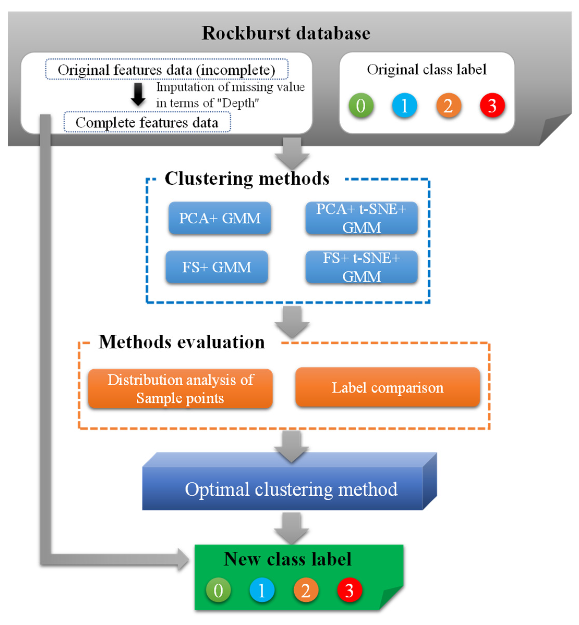
2.3. Relabeling of Original Data

The label of each sample signifies the rockburst intensity, determined using practical rockburst characteristics, which include features such as spalling or slabbing, failure depth, and the sound of a rockburst [42,43,44]. The total rockburst grades are commonly set to four; however, the definition of each grade may exhibit inconsistency due to differences in eras, countries, and individual perceptions. In this study, four classical rockburst proneness indices (Case 1–Case 4 in

Table 3. Different methods for relabeling the original data.

	Case 1	Case 2	Case 3	Case 4	Case 5	Case 6	Case 7	Case 8
Relabeling method	Russenes criterion	E.Hoek criterion	Wet	B1	PCA + GMM	PCA + t-SNE + GMM	FS + GMM	FS + t-SNE + GMM

) are used to validate the accuracy of the original class labels. The explicit expressions and corresponding criteria for these indices are presented in

Table 4. Four classical rockburst proneness criteria.

	Russenes Criterion	E.Hoek Criterion	Wet	B1
None rockburst	σθ/σc < 0.2	σθ/σc < 0.42	Ee/Ep < 2	σc/σt < 10
Light rockbust	0.2 ≤ σθ/σc < 0.3	0.42 ≤ σθ/σc < 0.56	2 ≤ Ee/Ep < 3.5	10 ≤ σc/σt < 14
Moderate rockburst	0.3 ≤ σθ/σc < 0.55	0.56 ≤ σθ/σc < 0.7	3.5 ≤ Ee/Ep < 5	14 ≤ σc/σt < 18
Strong rockburst	0.55 ≤ σθ/σc	0.7 ≤ σθ/σc	5 ≤ Ee/Ep	18 ≤ σc/σt

.

The new classification results based on each proneness index are shown in Figure 3. The results reveal that the original class labels agree with the new classification results for most indices to a certain extent. However, a notable number of samples demonstrate inconsistencies, particularly those samples that were originally classified as classes 1 and 2. Moreover, different indices result in distinct classification results. Therefore, it is evident that the original class labels of samples in the dataset might not have been determined based on a uniform criterion. This inconsistency significantly impacts the performance of the machine learning model. Hence, it is necessary to relabel the original data to ensure a more accurate and reliable classification.

Considering the limitations of the empirical proneness indices mentioned above, this paper integrates dimensionality reduction methods and clustering methods to carry out the relabeling process. The overall process of relabeling is illustrated in Figure 4, with the corresponding explanations presented as follows.

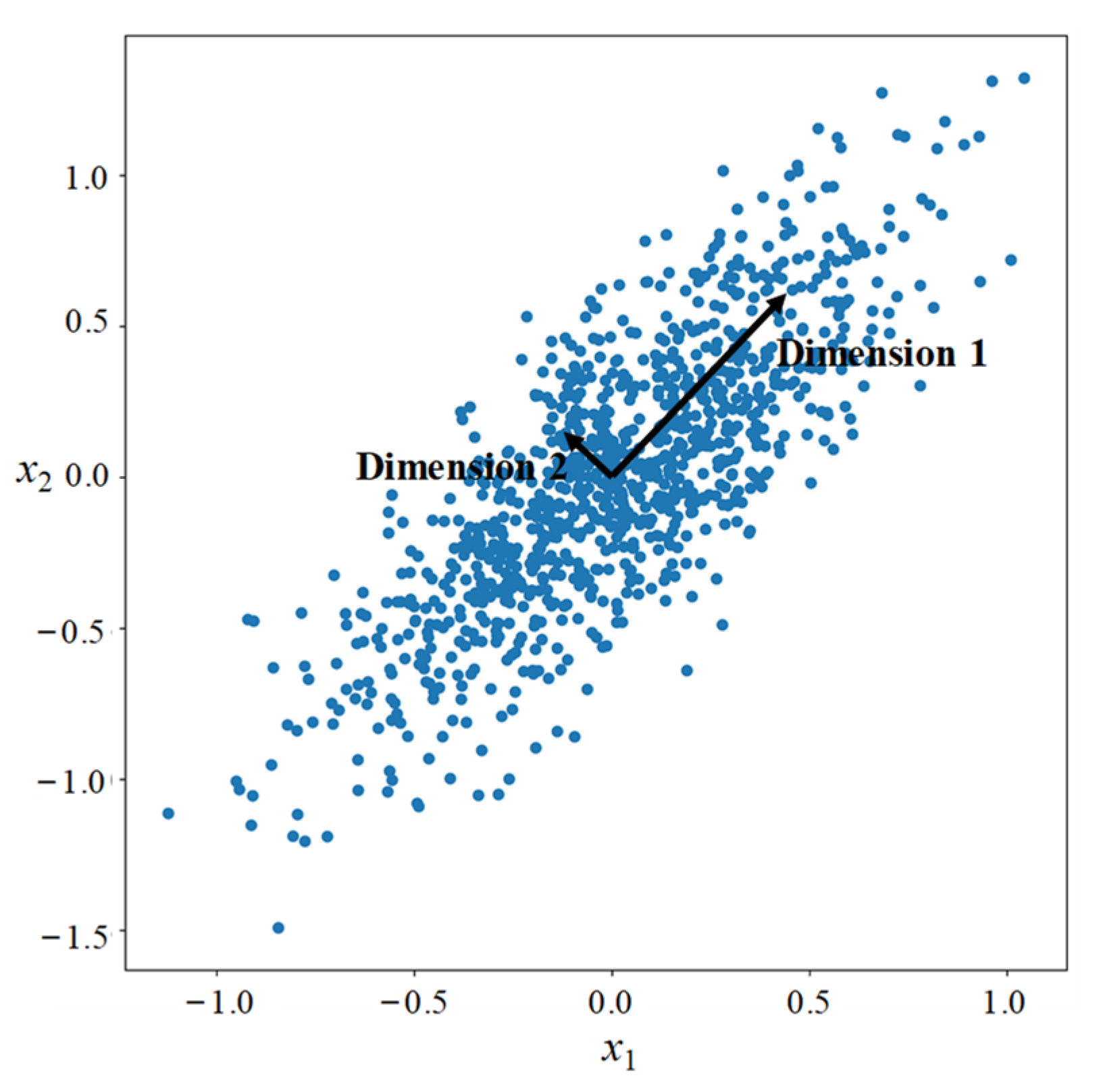
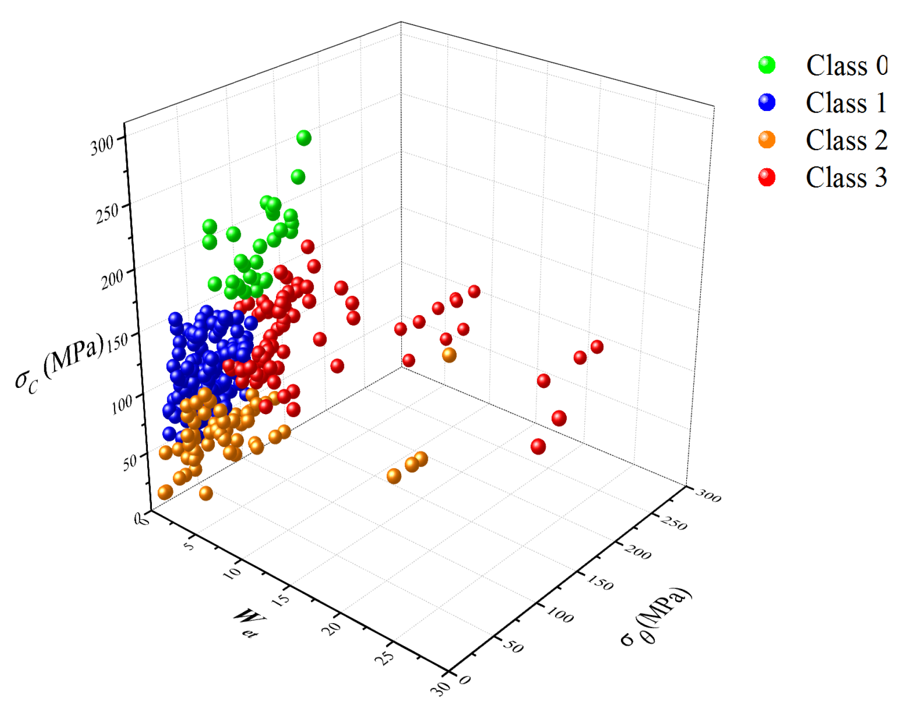
2.3.1. Dimensionality Reduction and the Clustering Method

Generally, samples that belong to the same class exhibit higher similarity, implying that they are more closely distributed in feature space. Clustering serves as an effective unsupervised learning method to achieve classification based on the sample distribution. Moreover, when dealing with datasets with a large number of features, appropriate dimensionality reduction becomes crucial. In this paper, four combination methods (Case 5–Case 8 in Table 3) for dimensionality reduction and clustering are developed and evaluated. For this purpose, PCA, t-SNE, and GMM were performed in Python using the scikit-learn library [45], thereby facilitating efficient and accurate data analysis.

• Principal Component Analysis (PCA)

PCA is a widely used dimensionality reduction method that transforms the original coordinate space into a new orthogonal space (Figure 5) [46,47]. The original coordinates of feature points are noted X (x₁, x₂…, x_m), with a size of n × m, where n represents the number of features and m represents the number of points. During PCA processing, X is initially mapped to the matrix A using min–max normalization. The values of the elements in A (a₁, a₂…, a_m) lie within the range of [0, 1]. Next, a decentralization matrix B is obtained by subtracting $\overline{A}$ (the mean of A along the row direction) from A, as indicated in Equation (1). Subsequently, the new coordinates X_pca of feature points can be calculated using Equation (2), where U is composed of eigenvectors of covariance matrix S of B. The components (or factor loadings) u_i of U can be computed using Equation (3), and the components (u₁, u₂…, u_n) are assigned successively based on the eigenvalues (or variances) of the covariance matrix S. Notably, the first component of X_pca captures the largest variance, thus retaining the most pertinent information of the samples in the initial dimensions.

In this study, the original rockburst dataset is processed using PCA. Based on the calculated eigenvalues, it is observed that the first five components account for 94% of the variance information in the samples. Specifically, 42% is attributed to the first component (F1), 21% to the second component (F2), 18% to the third component (F3), 7.3% to the fourth component (F4), and 5.6% to the fifth component (F5), thus establishing their significance.

The factor loadings were plotted in two-dimensional spaces (F1–F2, F2–F3, F3–F4, F4–F5), and the correlation coefficient matrix between the initial features and the scores on PCA factors is also presented. These visualizations and detailed information can be found in Supplementary Materials Figure S1 and Table S2, which reveal how each feature contributes to the principal components. Upon analyzing the correlation coefficient matrix, it becomes evident that the first five factors show significant linear relationships with specific features. In fact, the maximum absolute value of the correlation coefficient exceeds 0.6. Consequently, the features that contribute the most to each component are identified, as listed in

Table 5. Features with maximum absolute value of loadings for the first five components.

	F1	F2	F3	F4	F5
Feature	σt	σc	σθ	D	Wet

.

For a deeper understanding of the roles of features in relation to the principal components, a varimax rotation was performed. The loading matrix involving the rotated factors and the correlation coefficient matrix between initial features and scores on rotated factors are provided in Supplementary Materials Tables S3 and S4. In this case, the rotated factors are denoted RF1, RF2, RF3, RF4, and RF5. From this analysis, it is evident that certain features exhibit strong associations with the rotated factors, as in

Table 6. Features with strong correlation to the rotated factors.

	RF1	RF2	RF3	RF4	RF5
Factor	σt, B1, B2	σc	σθ, SCF	Wet	D

. Notably, features such as σ_t, B₁, and B₂ are highly aligned with RF1, which can be attributed to the marked negative correlation between σ_t and B₁ and B₂, as depicted in Figure 1. A similar trend is observed in relation to RF3. Taking both Table 5 and Table 6 into comprehensive consideration, it can be deduced that σ_t, σ_c, σ_θ, D, and W_et are the primary contributors to the principal components.

Furthermore, the Supplementary Materials show the factor scores on the principal components (Supplementary Materials Figure S2), it can be observed that the distribution of feature points becomes progressively denser from F1 to F5, indicating the efficacy of the PCA procedure.

In Case 5 (PCA + GMM), the original eight features are directly reduced to three dimensions using PCA to visualize the dataset effectively. In Case 6 (PCA + t-SNE + GMM), the original eight features are first reduced to five dimensions using PCA, and then further reduced using t-SNE with the same dimensionality reduction function.

$$B=A-\overline{A}=A-\frac{1}{m}{\displaystyle \sum _{i=1}^m{a}_i}$$

(1)

$$X_{pca}=U^T\cdot B$$

(2)

$$\{\begin{array}{l}{\widehat{u}}_i=\arg \max (u_i^{T}S{u}_i)\hfill \\ s.t.\hspace{1em}{u}_i^T{u}_i=1\hfill \end{array}$$

(3)

2.

Feature Selection (FS)

FS aims to identify influential and relatively independent features based on their physical meaning. Among the eight features mentioned above, SCF, B₁, and B₂ are expressed as functions of σ_θ, σ_c, and σ_t, respectively. Therefore, the former three features are initially eliminated. The buried depth D mainly influences the stress state of the surrounding rock; however, σ_θ provides more explicit information. Additionally, given the occurrence of missing values for D in some practical engineering cases, features associated with stress tend to favor selecting σ_θ over D. Considering that rockbursts often occur due to the extremely high compression stress that exceeds a rock’s capacity, σ_t has little effect on rockburst prediction. Consequently, σ_θ, σ_c, and W_et are selected as the ultimate dominant features. Here, σ_θ and σ_c reflect the possibility of rockburst, in other words, the closer σ_θ approaches σ_c, the greater the likelihood of rockburst occurrence. On the other hand, W_et reflects the hazard degree of rockburst; that is, a higher W_et value signifies a greater release of energy when a rockburst takes place.

3.

t-distributed Stochastic Neighbor Embedding (t-SNE)

t-SNE [48] is another dimensionality reduction method, distinguished by its remarkable capability to visualize high-dimensional data within an embedded space. This method transforms the affinities of sample points to probabilities using Student’s t-distributions. It facilitates optimizing the arrangement of data points in the new low-dimensional space, meticulously capturing their similarities and relationships in the original high-dimensional space. The new coordinates of feature points (z₁, z₂…, z_m) in low-dimensional space can be derived by minimizing the Kullback–Leibler (KL) divergence, also known as relative entropy, as expressed in Equation (4). In this equation, P_j|i (Equation (5)) represents the conditional probability affinity of the jth point given the ith point in the original high-dimensional space, while q_j|i (Equation (6)) represents the conditional probability affinity of the jth point given the ith point in the low-dimensional space. The relative entropy quantifies the disparity between two probability distributions (P_j|i and q_j|i). As q_j|i approaches P_j|i, the relative entropy diminishes, aiding in the retention of inherent similarities and correlations among feature points in the new low-dimensional space.

$$({\widehat{z}}_1,{\widehat{z}}_2\cdots {\widehat{z}}_m)=\underset{z_1,z_2\cdots z_m}{\mathrm{argmin}} {\displaystyle \sum _i^m{\displaystyle \sum _j^m{P}_{j|i}\ln \frac{P_{j|i}}{q_{j|i}}}}$$

(4)

$$P_{j|i}=\frac{e^{-{\Vert x_i-x_j\Vert }^2}}{{\displaystyle \sum _{k\ne i}{e}^{-{\Vert x_i-x_k\Vert }^2}}}$$

(5)

$$q_{j|i}=\frac{{(1+{\Vert z_i-z_k\Vert }^2)}^{-1}}{{\displaystyle \sum _{k\ne i}{(1+{\Vert z_i-z_k\Vert }^2)}^{-1}}}$$

(6)

In this method, similar samples are positioned in close proximity to enhance the clustering effect. In Case 6 (PCA + t-SNE + GMM) and Case 8 (FS + t-SNE + GMM), the data undergoes t-SNE processing and is presented as a three-dimensional form within the embedded space for visualization.

4.

Gaussian Mixture Model (GMM)

The GMM is an unsupervised clustering method, endowed with the capability to relabel samples based on the likelihood of their affiliation with each class. It assumes that samples stem from a mixture of a finite count (i.e., the number of classes K) of Gaussian distributions ϕ (x_i|μ_k, σ_k) (k = 1, 2…, K). Consequently, each sample holds an associated probability r_ik (i = 1, 2…, m) for each class. This ‘soft’ classification is more flexible than other ‘hard’ classification methods [34]. Moreover, r_ik is computed using the EM algorithm, and the relevant procedure is displayed in Algorithm 1.

Algorithm 1 EM algorithm in GMM.

Step 1 Initialize: Parameters of different Gaussian distributions {μk, σk, αk}, in which μk, σk, αk,k are the mean, variance, probability of kth Gaussian distribution respectively. Step 2 Update the probability rik that the ith sample belongs to kth Gaussian distribution: $\hspace{1em}\hspace{1em}{r}_{ik}=\left({\alpha }_k\varphi (x_i|{\mu }_k,{\sigma }_k)\right)/\left({\displaystyle \sum _{k=1}^K{\alpha }_k\varphi (x_i|{\mu }_k,{\sigma }_k)}\right)$. Step 3 Update the μk+1: ${\mu }_k=\left({\displaystyle \sum _{i=1}^m{r}_{ik}\cdot x_i}\right)/\left({\displaystyle \sum _{i=1}^m{r}_{ik}}\right)$. Step 4 Update the σk+1: ${\sigma }_k=\left({\displaystyle \sum _{i=1}^m{r}_{ik}(x_i-{\mu }_k){(x_i-{\mu }_k)}^T}\right)/\left({\displaystyle \sum _{i=1}^m{r}_{ik}}\right)$. Step 5 Update the αk+1: ${\alpha }_k=\left({\displaystyle \sum _{i=1}^m{r}_{ik}}\right)/m$. Step 6 If $\Vert {\mu }_{k+1}-{\mu }_k\Vert >{\epsilon }_{\mu }$, or $\Vert {\sigma }_{k+1}-{\sigma }_k\Vert >{\epsilon }_{\sigma }$, or $\Vert {\alpha }_{k+1}-{\alpha }_k\Vert >{\epsilon }_{\alpha }$:     Store the variables {μk+1, σk+1, αk+1};     Start the next iteration from Step 2.   Else if:     End the iteration.

2.3.2. Methods Evaluation

The clustering results obtained from the four combination methods are represented in Figure 6 and Figure 7. Before analyzing the results, it is important to clarify that the new cluster labels do not directly correspond to the original class labels. The meaning of the new cluster labels should be defined based on the sample distribution within each original class. Generally, a cluster with the maximum number of samples in a certain original class should be relabeled with the same class label. This relabeling process ensures that the new clusters represent similar rockburst intensities as the original class labels, enabling a more meaningful interpretation of the clustering results.

In Figure 6, it can be observed that most samples are clustered into two categories in Case 5, i.e., cluster 0 and cluster 2. A similar issue can be seen in Case 7. Figure 7a,c provides insights into understanding this peculiar situation, These figures represent the low-dimensional data space generated in Case 5 and Case 7, respectively, using dimensionality reduction methods.

In Case 5 and Case 7, the inherent Euclidean distance characteristics of sample points, with respect to the dominative feature dimensions, are preserved in the low-dimensional space. Consequently, certain sample points that are distant from the others are retained in a similar manner, resulting in the presence of outliers. Figure 8 illustrates these outliers across the three dominant feature dimensions of Case 7. As a consequence, these outliers either form a distinct cluster or are divided into two categories in Case 5 and Case 7. It is important to note that these outlier samples might have the same practical class as other normal samples. For instance, both high rockburst samples and extremely high rockburst samples belong to class 3. This scenario leads to misclassification and has an impact on the clustering accuracy.

The clustering effect in Case 6 and Case 8 seems to be satisfactory when observing Figure 7b,d. Taking into account the methodological variations, it can be concluded that the improved performance of Case 6 and Case 8 is largely attributed to the t-SNE process. This is because t-SNE transforms the Euclidean distance between sample points into probabilities, which in turn mitigates the impact of outliers. Based on the aforementioned relabeling regulation, where the maximum sample count determines the new class label, the new class label for each cluster in Case 6 and Case 8 is listed in

Table 7. The new class label for each cluster generated in Case 6 and Case 8.

New Class Label	Cluster in Case 6	Cluster in Case 8
0	3	0
1	2	1
2	1	3
3	0	2

.

To quantitatively compare the clustering effect between different cases, this paper uses the difference value of labels as the rejection score to measure the disparity between the original class label and the new class label (

Table 8. Rejection score of a sample for measuring the difference between the original label and the new label.

Original Class Label	New Class Label	Rejection Score
0	0	0
	1	1
	2	2
	3	3
1	0	1
	1	0
	2	1
	3	2
2	0	2
	1	1
	2	0
	3	1
3	0	3
	1	2
	2	1
	3	0

). A higher rejection score indicates less reliability of the relabeling method. Consequently, the rejection scores for the relabeling methods within each original class are listed in

Table 9. Rejection score in whole dataset for each case.

Class	Case 1	Case 2	Case 3	Case 4	Case 6	Case 8
0	51	25	50	88	57	57
1	103	69	69	137	93	39
2	71	151	96	119	100	106
3	40	97	12	93	58	55
Sum	265	362	227	437	297	257

along with the total rejection score. It is worth noting that Case 5 and Case 7 are excluded from the comparison since it was challenging to determine the new class label for outlier clusters based on the maximum sample number regulation for these two cases.

Table 9 indicates that the relabeling result using W_et (Case 3) is the closest to the original class label compared with the other three empirical proneness indices. However, it should be noted that an individual empirical proneness index can only reflect partial characteristics of rockburst, and thus, relying solely on a single feature for relabeling may lead to the loss of other valuable information from the dataset. Therefore, the comparison between Case 6 and Case 8 is expected to draw more attention.

In Table 9, it is evident that Case 8 outperforms Case 6. The relatively weaker relabeling ability of Case 6 can be attributed to PCA’s reliance on the distribution of sample points. To illustrate this, a simple example is provided in Figure 9, where the sample points are visualized in the σ_θ-W_et space, and two medium rockburst grades are marked as “Moderate I” and “Moderate II”. In the hypothetical distribution of sample points, as shown in Figure 9, the sample points within the “Moderate I” zone and the “Moderate II” zone are prone to be clustered into different categories after PCA processing. On the other hand, the sample points within the “None” zone and the “Strong” zone are more likely to be clustered into the same category with a high probability. In practical scenarios, it is crucial to distinguish the sample points within the “None” zone and the “Strong” zone. Consequently, PCA is susceptible to the distribution of sample points, while FS seems to offer more control and better results.

In summary, the FS + t-SNE + GMM combination method is selected as the optimal clustering method, and the original class labels of the samples are replaced with the new class labels generated using this method. The preprocessed dataset is used as input for the machine learning model to achieve the rockburst prediction.

3. Establishment of the Machine Learning Model

In order to reduce the sensitivity of a single model to the dataset, an ensemble strategy is used in this paper. Therefore, a voting ensemble model is used to predict rockburst, comprising five base learners (SVM, DT, LR, KNN, and NN). The implementation of these learners was conducted using Python with the scikit-learn library [45]. Furthermore, four optimization algorithms were utilized to determine the optimal hyperparameters of the base learners. This optimization process was executed in Python, using both the scikit-learn library and additional tools such as the scikit-opt library [49] and the optuna library [50]. The complete training and prediction workflow for the machine learning models is illustrated in Figure 10.

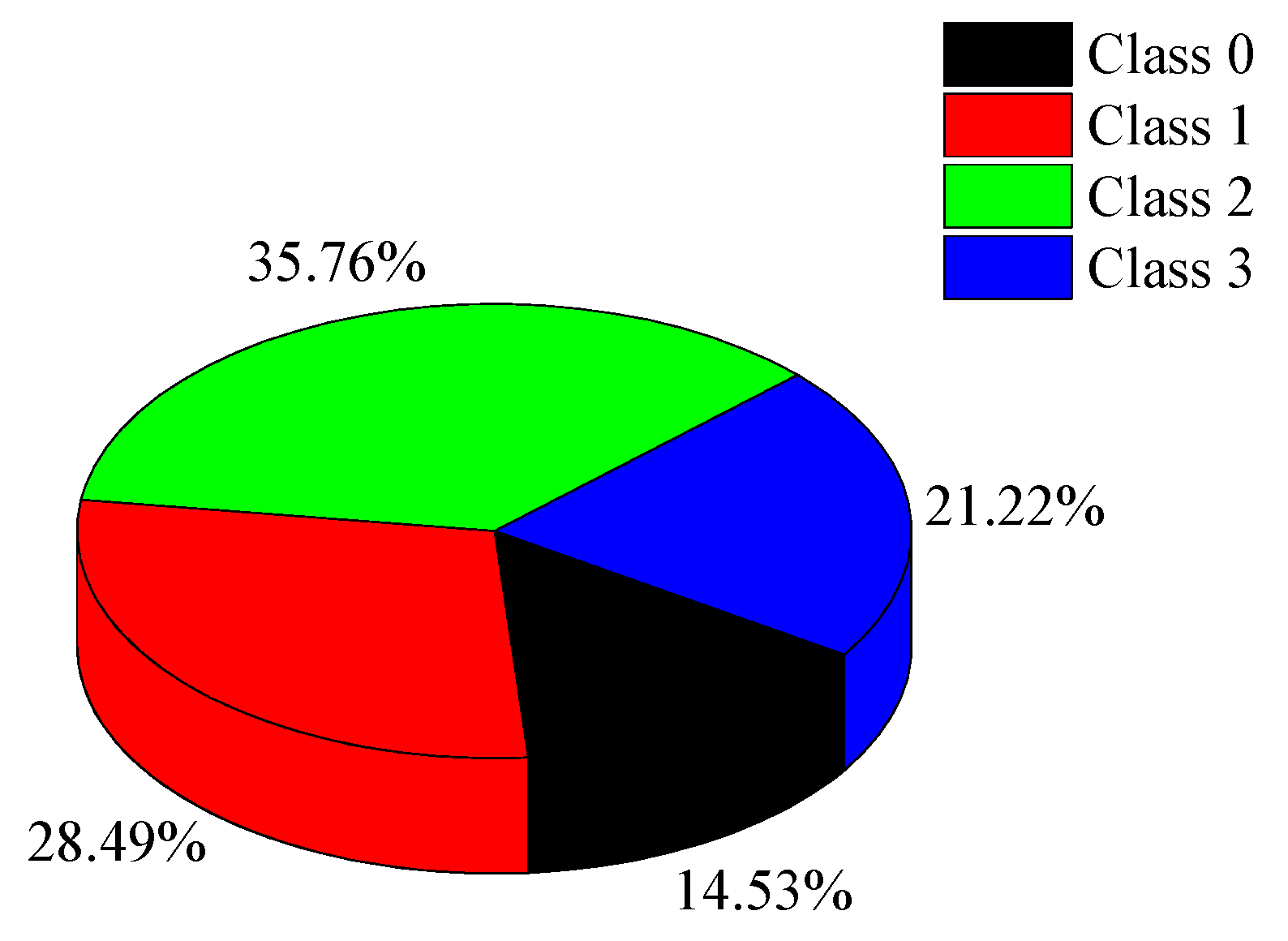
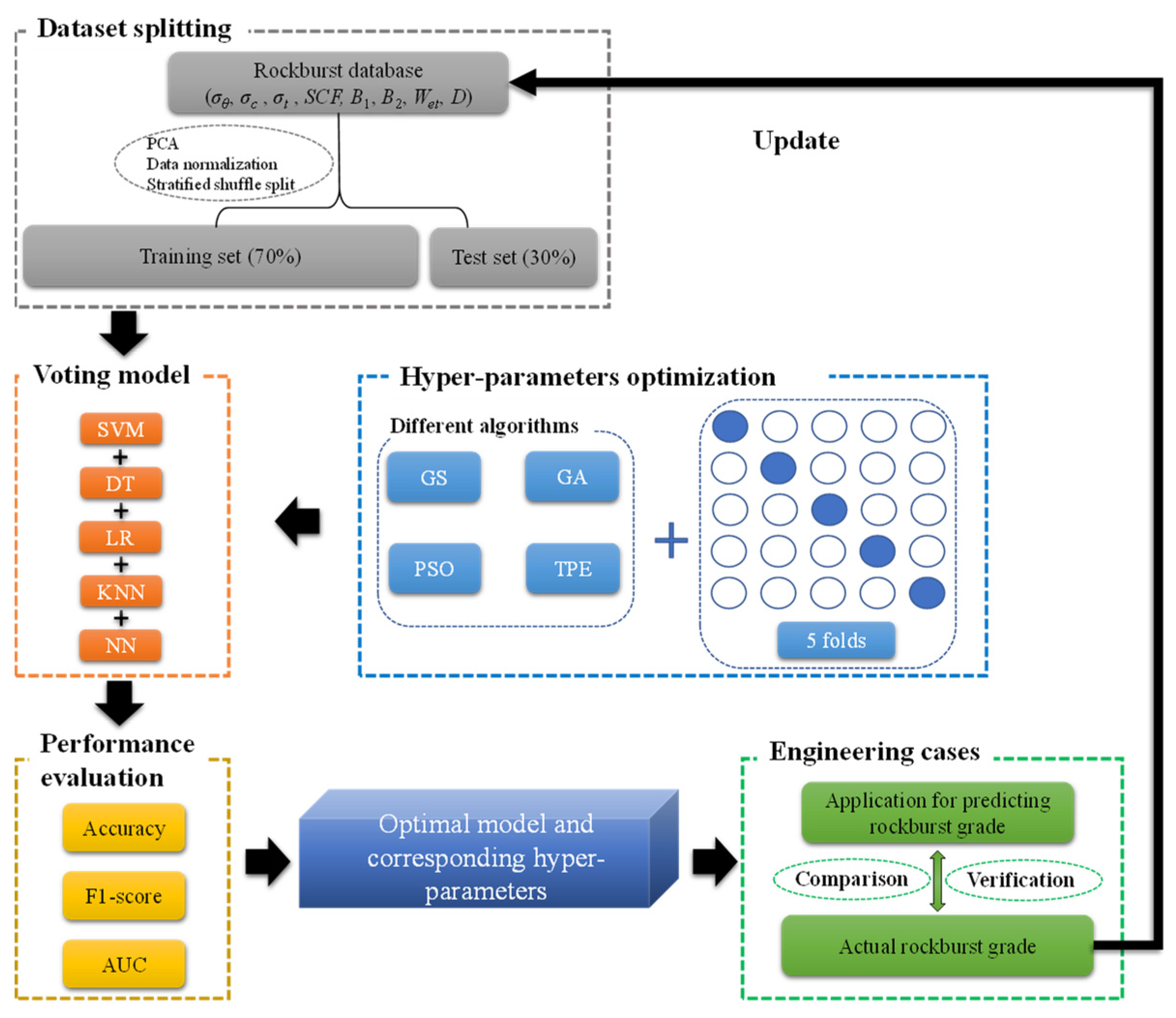
3.1. Dataset Splitting

During the training of a learner, dealing with a substantial number of features can potentially lead to an unnecessary proliferation of hyperparameters or even trigger overfitting of the model. Moreover, when features exhibit correlations, computational resources might be inefficiently utilized. To tackle these challenges, an initial PCA processing is applied to reduce the feature number and ensure a set of orthogonal components. Based on the earlier PCA analysis, it is evident that the primary five components encapsulate a significant portion of information extracted from the samples. This information encompasses what is reflected by the dominant features (σ_θ, σ_c, W_et) that are closely linked to rockburst occurrences. Consequently, the dimensionality of features is reduced to just five, allowing for more efficient and effective learning.

Moreover, the original features have different orders of magnitude, which can cause a prolonged training process and make the model difficult to converge. Therefore, data normalization processing is necessary to bring all features to a similar scale.

Subsequently, the dataset is split into two parts: a training set and a test set. The training set accounts for 70% of the dataset, while the test set accounts for 30% of dataset. To maintain consistency, the proportions of samples within each class in both sets are kept the same. This splitting process is achieved using stratified shuffle splitting.

3.2. Voting Ensemble Model

The voting model creates a comprehensive prediction by combining a limited number of base learners that belong to different types. Each base learner is trained using the same original dataset. These learners are independent of each other, allowing their prediction results to be determined using a majority vote strategy or an average probability strategy based on the outputs of multiple well-performing base learners. The ensemble strategy helps to reduce the potential overfitting of a single learner to the dataset, and it also alleviates the issue of unbalanced datasets. In this paper, five machine learning classifiers (SVM, DT, LR, KNN, and NN) are selected as the base learners for the voting method.

• Support Vector Machine (SVM)

SVM aims to find a hyperplane that can effectively classify or regress data points. The objective function of SVM reflects the distance between the hyperplane and the sample points and is convex, along with its constraint conditions. This convexity nature allows SVM to transform the inversion problem into a convex optimization problem, ensuring that a global optimal solution can be obtained in theory.

The mathematical expressions of the objective function and constraint conditions in SVM are shown in Equation (7). In this equation, w and b represent the slope and intercept of the hyperplane, respectively, and ξ_i and y_i stand for the slack variable and label of the ith sample point, respectively, and c is a hyperparameter that regulates the balance between maximizing the margin and minimizing the classification errors.

One of the strengths of SVM is its ability to use only a subset of the support vectors to determine the hyperplane rather than relying on all the data points. This feature leads to higher accuracy and computational efficiency. Furthermore, SVM can handle nonlinear problems effectively by utilizing kernel functions. In this paper, the radial basis function (RBF), as shown in Equation (8), is selected as the kernel function. In the equation, g represents another hyperparameter of SVM that governs the impact of the RBF kernel.

$$\{\begin{array}{l}\underset{w}{\min } \frac{1}{2}{\Vert w\Vert }^2+c{\displaystyle \sum _{i=1}^m{\xi }_i}\hfill \\ \mathrm{s}.\mathrm{t}. 1-y_i(w^T{x}_i+b)-{\xi }_i\le 0;{\xi }_i\ge 0\hfill \end{array}$$

(7)

$$k(x_i,x_j)=\exp \left(-g\cdot {\Vert x_i-x_j\Vert }^2\right)$$

(8)

b.

Decision Tree (DT)

In a classification problem, decision trees (DTs) split the dataset based on a predetermined feature criterion at a node. This process is designed to ensure that the entropy of the entire dataset decreases after each split. The tree continues to grow in this manner until it reaches the specified depth D_t, when the number of samples at each leaf node reaches the minimum value n_l, or when the number of samples at each split node reaches the minimum value n_s.

To measure the entropy after each split, this paper uses the Gini index, as shown in Equation (9). The Gini index calculates the impurity of a dataset after a split, where p_k is the probability that a sample in a leaf node belongs to the kth class (k = 1, 2…, K) according to a certain split scheme.

Once a decision tree is completed, the label of a new sample can be predicted by traversing the tree along one of its branch lines, where the identification of the sample at each leaf node can be considered a binary problem. Therefore, decision trees are computationally efficient, and their structure is easily visualized, making them easy to interpret.

$$Gini=1-{\displaystyle \sum _{k=1}^K{p}_k^2}$$

(9)

c.

Logistic Regression (LR)

LR is a widely used classifier for binary problems [51]. It models the probability of a sample belonging to a certain class using the logistic function, as shown in Equation (10). In this equation, the coefficients w_L are obtained using maximum likelihood theory, as represented in Equation (11), where C is the inverse of the regularization strength.

LR can also be extended to handle multiclass problems using the one-vs-rest strategy. In this approach, a separate binary classifier is trained for each class, treating it as the positive class, while the other classes are grouped together as the negative class. This way, LR can handle multiple classes by combining the results from each binary classifier.

$$P(y_i=1|w_L)=\frac{1}{1+e^{-w_L{}^T{x}_i}}$$

(10)

$${\widehat{w}}_L=\underset{w_L}{\arg \max } C{\displaystyle \sum _{i=1}^m\left(y_i\log (P)+(1-y_i)\log (1-P)\right)}$$

(11)

d.

K-Nearest Neighbor (KNN)

The fundamental idea of KNN is to estimate the class of a sample point by considering the majority vote class of its nearest neighbor points. The number of nearest neighbor points, denoted as n_k, needs to be specified manually beforehand. The distance d between two sample points is typically measured using Euclidean distance, as shown in Equation (12).

This straightforward logic ensures a fast training and prediction process, and its effectiveness has been validated in numerous practical cases [52,53,54]. KNN is particularly useful when dealing with non-linear and complex data patterns, and it does not require assumptions about the underlying data distribution. However, it may suffer from some limitations, such as sensitivity to noisy or irrelevant features and the need for careful selection of the appropriate value of n_k.

$$d=\Vert x_i-x_j\Vert$$

(12)

e.

Neural Network (NN)

An NN attempts to deduce the mapping relationship between an input layer (features) and an output layer (target) by incorporating one or more hidden layers, where the number of elements in the hidden layer is noted n_e. The usage of the activation function enables the model to handle non-linear relationships effectively. The coefficients (weights w_i and bias b_i) that connect layers are determined using the gradient descent method with a backpropagation process, as illustrated in Equation (13). In this equation, η represents the learning rate, and Loss is the loss function, expressed as Equation (14), which includes the term α||W||₂² for L2-regularization. In theory, an NN can simulate any non-linear relationship between features and a target, making it a powerful tool for complex modeling tasks.

$$\{\begin{array}{c}{w}_i{}^{(j+1)}=w_i{}^{(j)}-\eta \frac{\partial Loss}{\partial w_i}\\ b_i{}^{(j+1)}=b_i{}^{(j)}-\eta \frac{\partial Loss}{\partial b_i}\end{array}$$

(13)

$$Loss=-\frac{1}{m}{\displaystyle \sum _{i=1}^m{y}_i\ln {\widehat{y}}_i}+\frac{\alpha }{2m}{\Vert W\Vert }_2^2$$

(14)

3.3. Hyperparameters Optimization

Hyperparameters have a significant effect on machine learning models, and inappropriate settings can lead to low prediction accuracy or over-fitting. To find the optimal hyperparameters, various optimization algorithms have been designed and proven reliable. In this paper, we use four different algorithms (GS, GA, PSO, and TPE) to optimize the hyperparameters of the aforementioned base learners. While GS, GA, and PSO algorithms have been widely applied, the TPE algorithm is relatively scarce in the field of rockburst prediction. Therefore, we will provide a further introduction to the TPE algorithm in this section.

The TPE estimator belongs to the Bayes optimization method, which claims to fit the relationship between a target variable y and input variables X (x₁, x₂, …) and estimate the extreme point. The entire workflow of TPE in one iteration is shown in Figure 11. A step-by-step explanation of the process is given as follows: (1) TPE starts by assuming a prior distribution P(y) of the target variable y and randomly sampling several data points. (2) A surrogate function is then estimated using the kernel density estimation based on the previous P(y) and the sample data points. This surrogate function simulates the behavior of the objective function. The corresponding posterior distribution of the target variable P(y|X) is also derived. (3) Next, an acquisition function is deduced using the expected improvement method, which is based on the surrogate function and the posterior distribution P(y|X). The acquisition function helps to select the next point to evaluate in order to optimize the objective function. (4) The point with the maximum value of the acquisition function is added to the set of data points, and the process repeats with a new iteration based on the extended set of data points. This continues until the specified iteration number is reached.

The TPE algorithm efficiently searches for the optimal hyperparameters by iteratively updating the surrogate function and using it to guide the search for the extreme point. For more detailed information on TPE, readers are referred to Bergstra et al. [55].

The hyperparameters of different base learners that need to be optimized using optimization algorithms are listed in

Table 10. Hyperparameters of different classifiers and corresponding sampling scope for each optimization algorithm.

Classifier	Hyperparameters	Empirical Scope
SVM	Penalty coefficient c	[2−10, 210]
	Gamma in RBF kernel function g	[2−10, 210]
DT	Maximum depth of tree Dt	[3, 15]
	Minimum number of samples at leaf node nl	[1, 10]
	Minimum number of samples at split node ns	[2, 10]
LR	Inverse of regularization strength C	[0.01, 50]
KNN	Number of neighbors nk	[3, 15]
	Weight strategy	“Uniform” or “Distance”
NN	Number of elements in hidden layer ne	[5, 15]
	Strength of the L2 regularization α	[0.00001, 1]
	Initial learning rate η	[0.0001, 0.5]

, along with their corresponding sampling scopes.

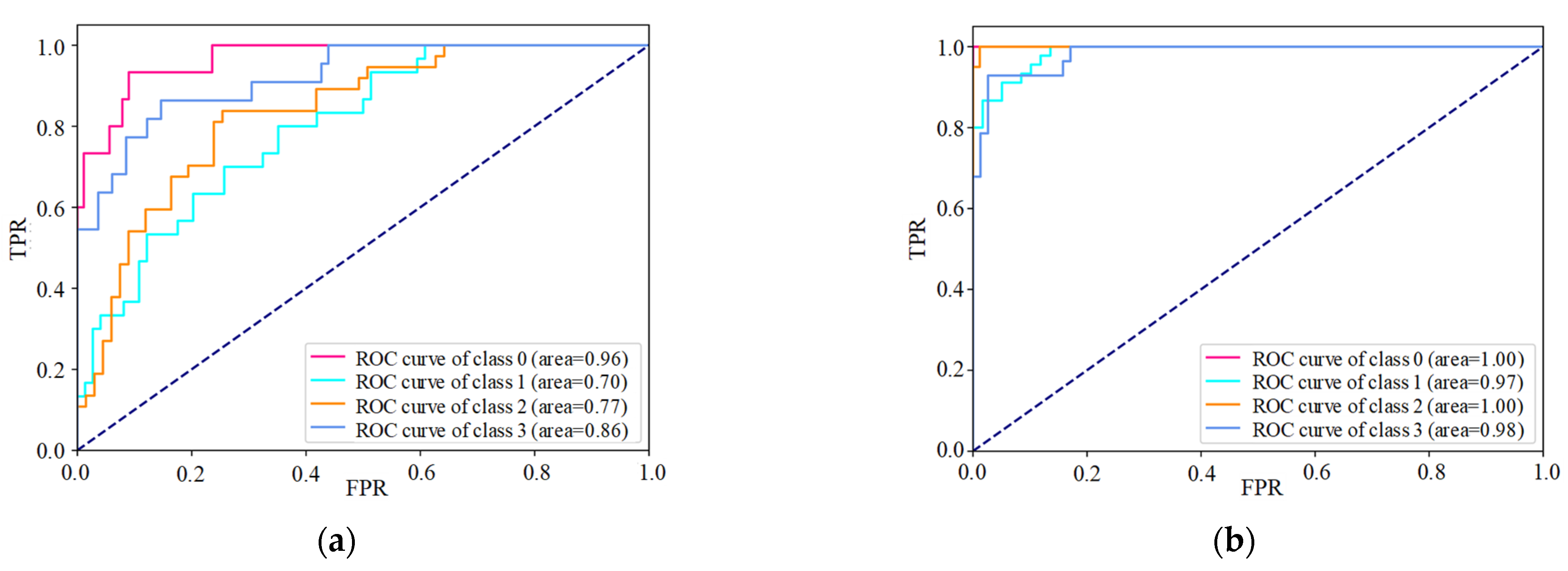
4. Results of Prediction and the Performance Evaluation

This paper intends to confirm the optimal combination model and also validate the effect of the FS + t-SNE + GMM relabeling method. Therefore, two datasets are used to construct the machine learning models: one with the original label and another with the new label obtained using the FS + t-SNE + GMM relabeling method.

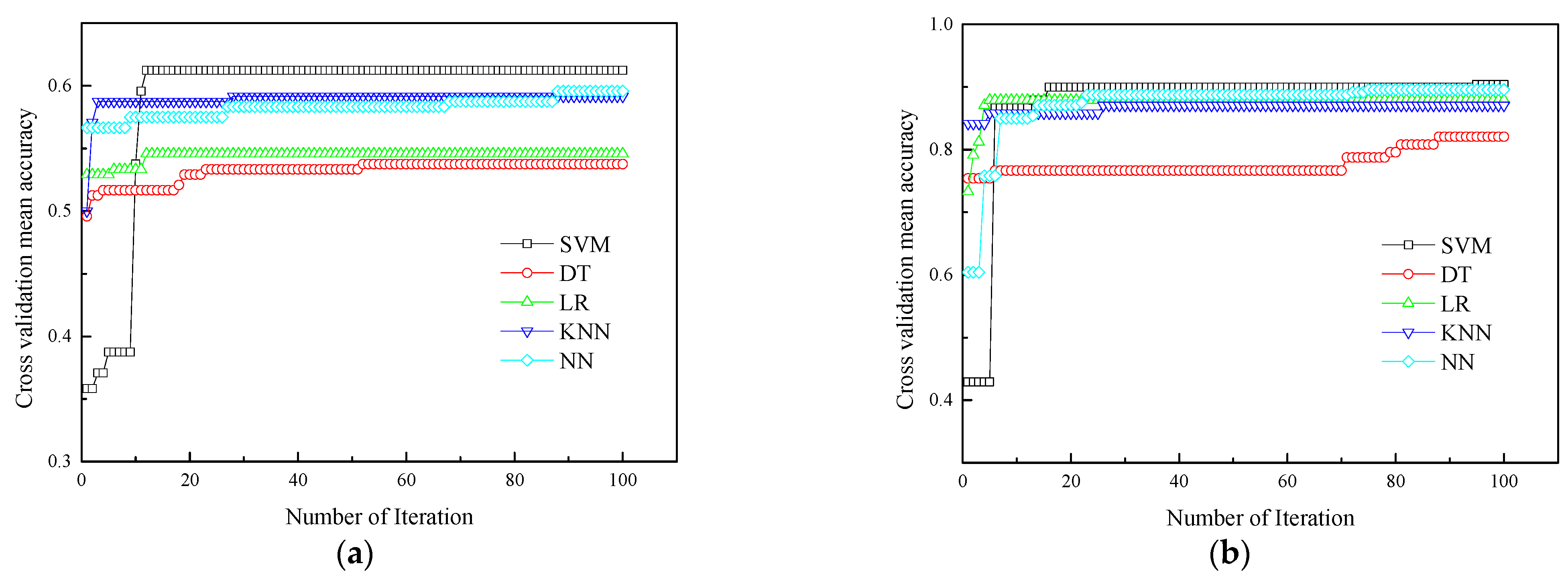
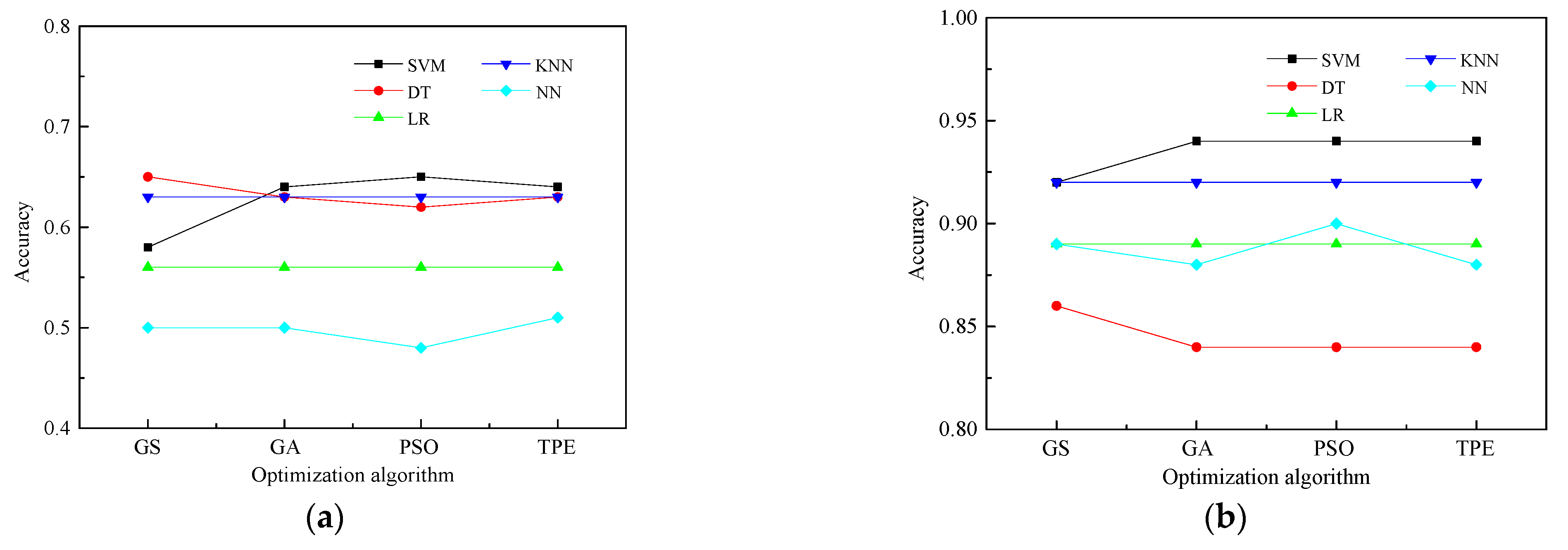
4.1. Results of Hyperparameter Optimization

In order to derive the optimal hyperparameters of base learners, each optimization algorithm is used in conjunction with five-fold cross-validation (Figure 10). Figure 12 displays the variation in mean prediction accuracy using the validation set with each iteration. For the dataset with the original labels, the final accuracy ranges from approximately 50% to 60% for each base learner. On the other hand, for the dataset with the new labels, the final accuracy consistently remains around 90%. Moreover, the variation curves for the two different datasets also reveal that the accuracy improves gradually and stabilizes toward the end of the iterations. These observations confirm that the models progressively approach the optimal solution. The hyperparameter combination scheme with the highest accuracy for the validation set is considered optimal. The optimal hyperparameter scheme for each learner is listed in

Table 11. Optimal hyperparameters for different machine learning models obtained using optimization algorithms.

Classifier	Hyperparameter	Dataset with Original Label				Dataset with New Label
		GS	GA	PSO	TPE	GS	GA	PSO	TPE
SVM	c	2000.00	3.93	3.21	32.02	2.00	67.70	69.26	100.48
	g	0.20	9.34	9.40	9.38	20.00	5.21	5.11	4.22
DT	Dt	10.00	14.00	12.00	13.00	8.00	12.00	13.00	10.00
	nl	5.00	4.00	7.00	8.00	2.00	2.00	2.00	2.00
	ns	7.00	5.00	4.00	5.00	2.00	4.00	2.00	5.00
LR	C	6.10	4.96	5.00	4.90	32.66	32.13	34.19	32.70
KNN	nk	9.00	9.00	9.00	9.00	5.00	5.00	5.00	5.00
	Weight strategy	distance	distance	distance	distance	distance	distance	distance	distance
NN	ne	7	10	5	10	9	10	12	8
	α	10−4	0.05	0.75	0.61	0.001	0.14	10−5	0.01
	η	0.13	0.12	0.06	0.03	0.13	0.02	0.10	0.11

.

The time elapsed when searching for the optimal solution and the accuracy of prediction for the test set are two crucial indices for evaluating the performance of the optimization algorithm. Figure 13 and Figure 14 display a performance comparison among the different algorithms in terms of these two aspects.

Figure 13 shows that the optimization time when using GA and PSO is susceptible to the machine learner. For some learners, such as LR and NN, the hyperparameter optimization process requires an enormous amount of time using GA and PSO. By contrast, GS and TPE are characterized as having more efficiency. However, the search time when using GS mainly depends on the number of features and the search interval. In other words, when the feature count is large and the search interval is small, GS also requires much time. On the other hand, Bayes optimization enables TPE to search in a direction of expected improvement, thereby saving a lot of time compared with GA and PSO.

Figure 14 shows that the accuracy results of a machine learner combined with different optimization algorithms have few differences between them, which indicates that the four optimization algorithms are capable of finding a good hyperparameter combination. In summary, the abilities of the four optimization algorithms in searching for the optimal solution are similar, but TPE stands out as the fastest and most efficient algorithm among them.

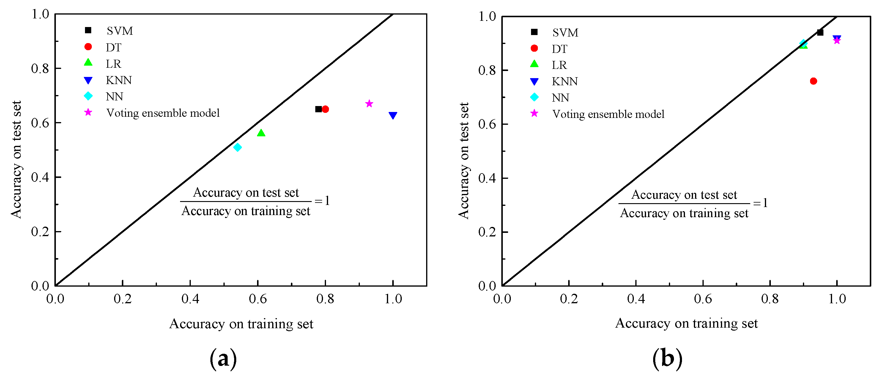
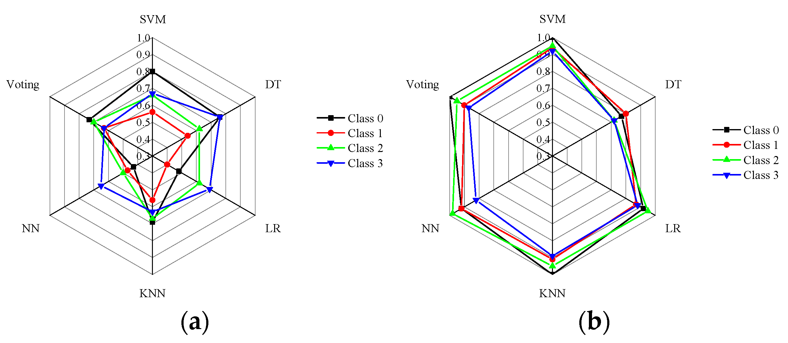
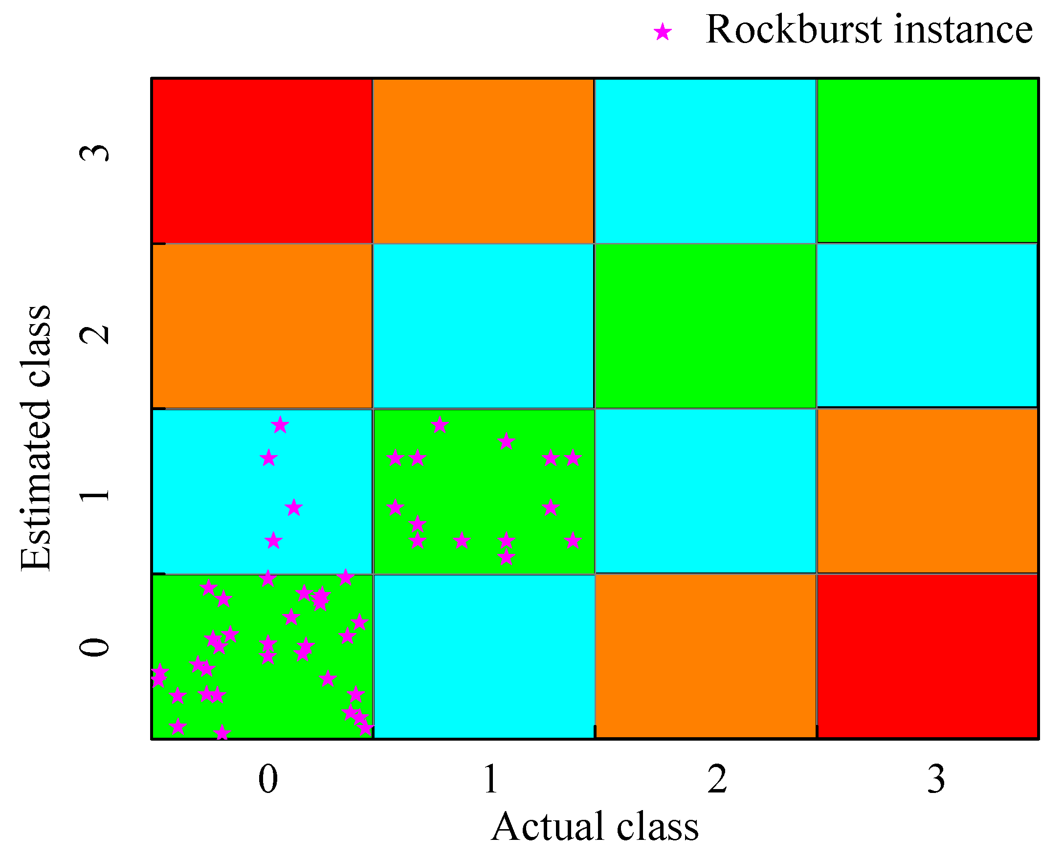
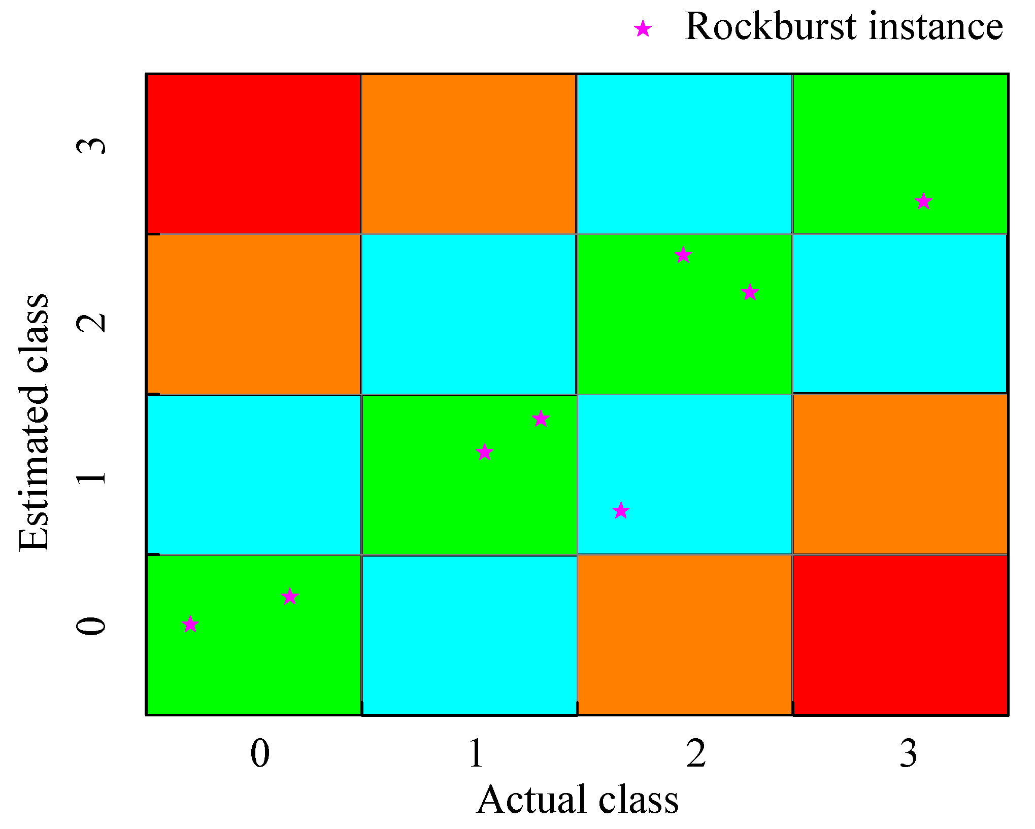
4.2. Prediction Results of the Machine Learning Model

After hyperparameter optimization, the machine learning model was trained and used to estimate the class of samples. The prediction accuracy for each base learner and the ensemble model using the training set and test set is displayed in Figure 15. It can be observed that the accuracy based on the dataset with the original label is limited to about 70% (Figure 15a), while the accuracy based on dataset with the new label can reach 90% (Figure 15b). Additionally, the scatter points in Figure 15b closely approximate the line (accuracy on training set = accuracy on test set), indicating that the preprocessing of the dataset regarding the original label improves not only the prediction accuracy but also the generalization ability.

Furthermore, in terms of the raw dataset, the voting model outperforms most single learners. Moreover, when it comes to a high-quality dataset, some single learners perform as well as the voting model or even slightly better. In general, the voting method demonstrates a relatively good prediction accuracy on both datasets, making it a favorable choice, especially in the cases where sufficient understanding of a dataset is lacking.

In addition to accuracy, there are other metrics that measure the quality of prediction for each class, such as precision, recall, F1-score, and the receiver operating characteristic curve (ROC) [27,32,35,36]. Precision reflects the credibility of the prediction result using a classifier for a certain class, while recall represents the ability of a classifier to find all relevant samples belonging to a certain class. The F1-score can be regarded as the harmonic mean of precision and recall. An ROC displays the relationship between the false positive rate (FPR) and the true positive rate (TPR) for a certain class, and the area under the curve (AUC) can be used to measure the accuracy for that class, where a higher AUC indicates higher accuracy.

The values of the F1-score for the dataset with the original label and the dataset with the new label are displayed in Figure 16. Additionally, the ROC curves for each class, both for the dataset with the original label and the dataset with the new label, are shown in Figure 17.

Based on the comprehensive metrics (F1-score and AUC), in Figure 16 and Figure 17, it is evident that the voting model still outperforms most single learners. Furthermore, when considering the dataset with the original label, the prediction on class 0 exhibits the highest accuracy, followed by class 3, class 2, and class 1, respectively. However, considering the dataset with the new label, the prediction on class 0 also demonstrates the highest accuracy, followed by class 2, class 1, class 3, in that order. Therefore, preprocessing the dataset enhances the ability to identify class 1 and class 2 accurately.

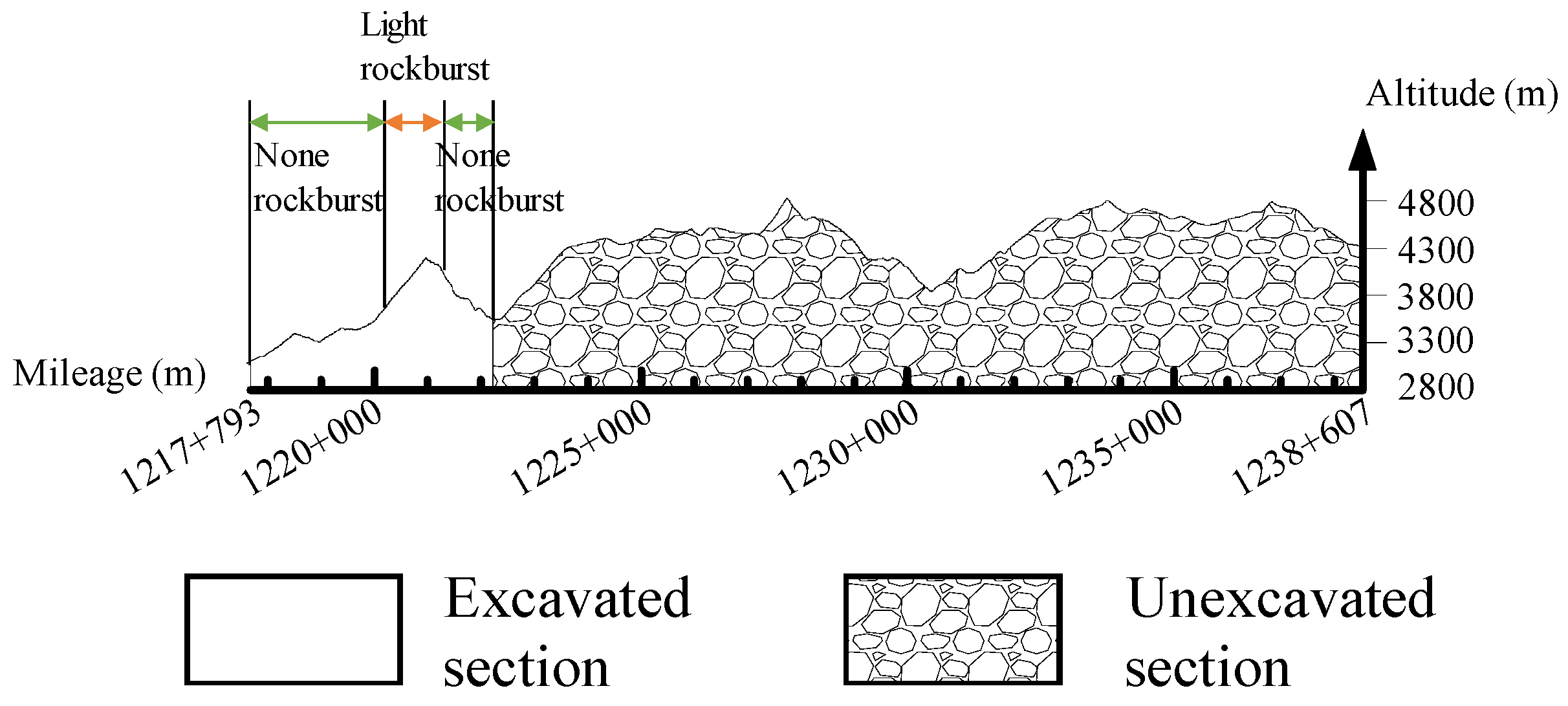
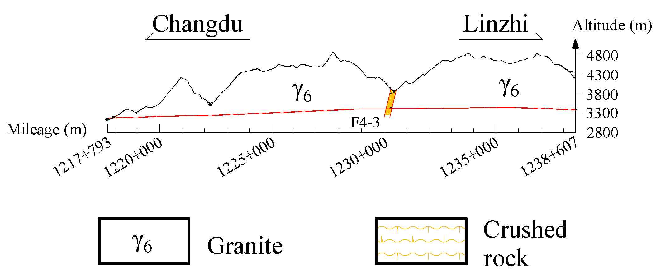
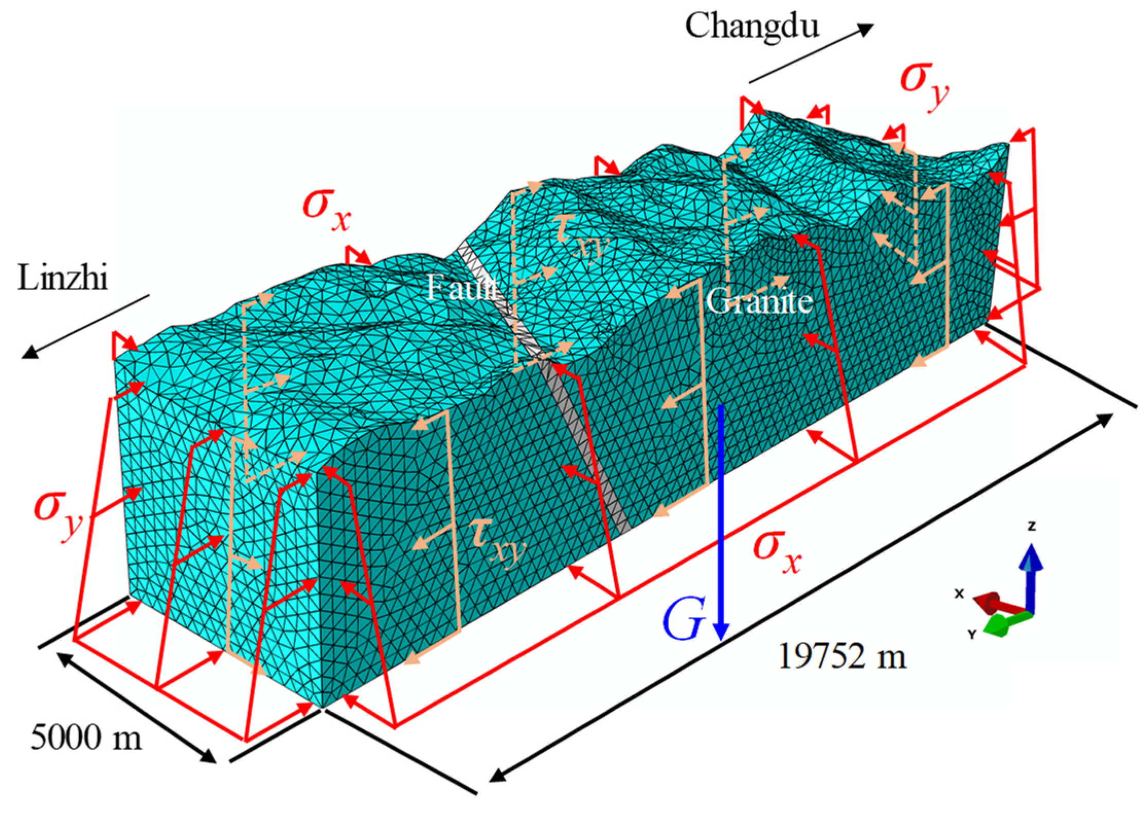
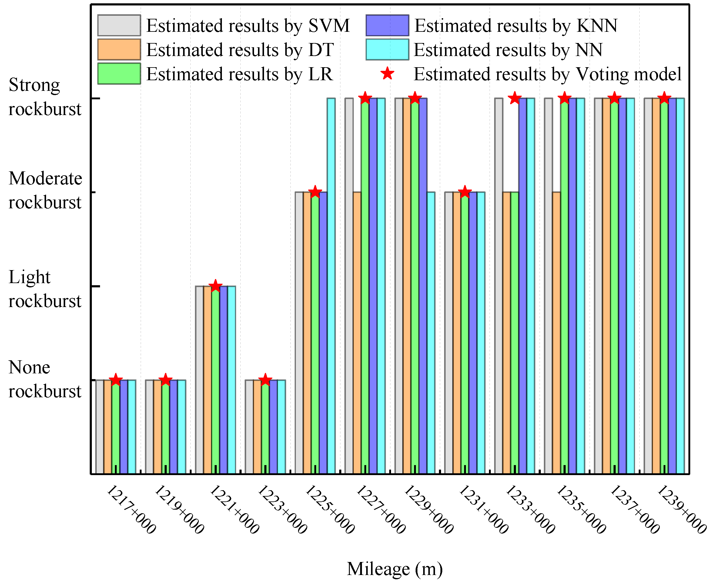
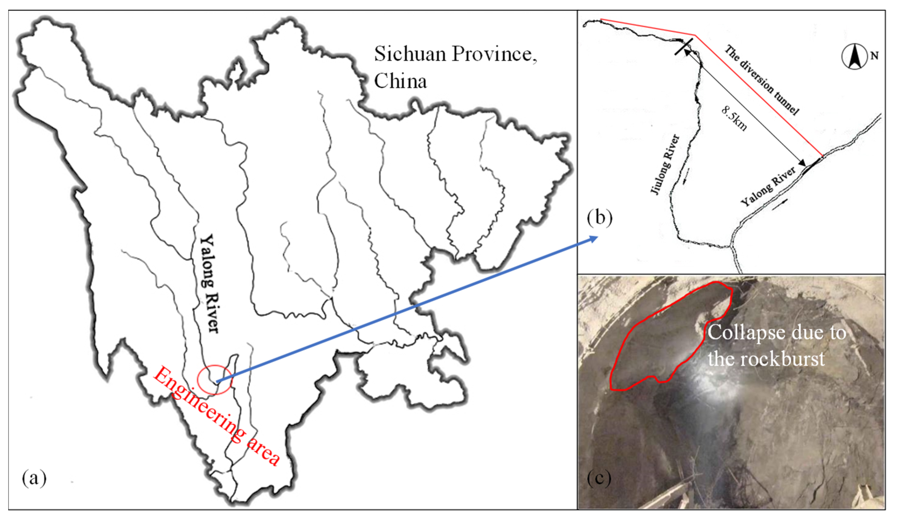
5. Validation on Practical Engineering Case

Based on the performance evaluation, the model combining the voting method and TPE optimization algorithm is considered stable and efficient with high prediction accuracy. As a result, this model is chosen as the optimal approach for conducting rockburst prediction in practical engineering cases.

5.1. Case 1

The engineering case used for validation is a superlong (37,965 m) and deep buried tunnel located in the Gangdese orogenic belt in the Tibet Autonomous Region, China. Construction of the tunnel began in January 2021. The tunnel site has experienced impacts from the Neo-Tethys oceanic plate and the Indian oceanic plate, resulting in the principal stress field being NE-SW or NEE-EW. The tunnel passes through numerous mountains, with a maximum burial depth of 1680 m.

Given its superlong length, large burial depth, and significant tectonic stress, the construction of this tunnel is highly challenging. Additionally, the granite section, spanning approximately 20 km, poses a severe risk of rockbursts. Figure 18 displays the profile of the tunnel site and the strata situations, in which the horizontal axis represents tunnel mileage, and the vertical axis represents the altitude. Here, to validate the proposed combination model, an excavated section near the entrance, approximately 4 km in length, is used in the validation process.

The input data for the model includes the feature σ_θ, which is obtained with in situ stress inversion using numerical and regression methods [56,57]. During the inversion process, a topographic model of the tunnel site area is established using the GIS method, as illustrated in Figure 19. The study area covers a mileage range from 1218 + 855 m to 1238 + 607 m, with a length of 19,752 m and a width of 5 km. The height of the free surface is determined using the altitude of each point.

The topographic model was incorporated into ABAQUS software to construct the finite element numerical model. The mechanical parameters utilized in the numerical model were obtained using indoor rock tests, as detailed in

Table 12. Mechanical parameters of the materials in the numerical model.

Lithology	Density ρ (g/cm3)	Young’s Modulus E (GPa)	Poisson’s Ratio μ	Cohesion Yield Stress C (MPa)	Friction Angle φ (°)
Granite	2.7	23.53	0.27	2	56
Fault	2.63	12	0.35	0.6	35

. The material constitutive relation follows the Mohr–Coulomb elastic-plastic model.

The encastre constraint was applied to the bottom boundary, while the top surface was set as free. The vertical principal stress of the strata was represented by gravity, while the lateral stress boundary conditions were governed by the horizontal principal stresses of the strata, namely, the horizontal maximum principal stress σ_H and the horizontal minimum principal stress σ_h. Following the findings of Brown and Hoek [58] regarding the relationship between in situ stress and burial depth D, σ_H and σ_h were expressed using Equations (15) and (16), respectively. The constants k_H, b_H, k_h, and b_h in these equations needed to be determined using regression based on measured in situ stress data. SVM regression was used for this purpose. Notably, the stresses applied to the lateral side of the model were σ_x, σ_y, and τ_xy, rather than σ_H and σ_h. Their relationships were expressed using Equations (17)–(19), where φ represents the angle between σ_H and the tunnel axis (direction of the y-axis). Based on actual measurements obtained by drilling at the tunnel site, φ was found to be approximately 10°. The comprehensive boundary conditions are also illustrated in Figure 19.

$${\sigma }_H=k_H\cdot D+b_H$$

(15)

$${\sigma }_h=k_h\cdot D+b_h$$

(16)

$${\sigma }_x=\frac{{\sigma }_H+{\sigma }_h}{2}-\frac{{\sigma }_H-{\sigma }_h}{2}\cdot \cos 2\phi$$

(17)

$${\sigma }_y=\frac{{\sigma }_H+{\sigma }_h}{2}+\frac{{\sigma }_H-{\sigma }_h}{2}\cdot \cos 2\phi$$

(18)

$${\tau }_{xy}=\frac{{\sigma }_H-{\sigma }_h}{2}\cdot \sin 2\phi$$

(19)

After the in situ stress inversion, σ_θ was deduced using Equation (20) based on elastic theory, where σ_x and σ_z represent the horizontal and vertical stress of the tunnel element, respectively. The values of σ_θ along the tunnel are shown in Figure 20.

$${\sigma }_{\theta }=2\cdot ({\sigma }_z+{\sigma }_x)+2\cdot \left|{\sigma }_z-{\sigma }_x\right|$$

(20)

The features σ_c, σ_t, and W_et are determined using indoor mechanical tests on the granite samples of tunnel site, and their values are listed in

Table 13. Value of σ_c, σ_t, and W_et regarding the rock surrounding the tunnel.

σc (MPa)	σt (MPa)	Wet
150	4.82	3.82

. The values of SCF, B₁, and B₂ can be calculated according to their respective definitions, and the buried depth D can be determined as described in Figure 18.

The mentioned eight features are inputted into the machine learning model to estimate the rockburst grade along the tunnel, as illustrated in Figure 21. To demonstrate the composition of the voting model, the estimated outcomes using specific five base learners are also depicted in Figure 21. Additionally, 53 instances of rockburst along the tunnel were measured and recorded to evaluate the prediction results. The actual rockburst situation is visualized in Figure 22, and a detailed comparison is presented in a cross-plot (Figure 23), offering a comprehensive post-validation of the model.

The accuracy of the proposed model is reflected by the distribution of points in the diagonal zones (green zones) within the cross-plot. Notably, only four instances were overestimated in the prediction results, being classified as a light rockburst grade, while the actual occurrences showed no rockburst events. However, the majority instances were accurately estimated, yielding a remarkable accuracy rate of 92%. This showcases the robustness and reliability of the proposed combination model.

5.2. Case 2

The diversion tunnel of Jiangbian Hydropower Station serves as the engineering case in this study, which is situated alongside Jiulong River in Sichuan Province, China (Figure 24a,b). The tunnel has a diameter of 8.4 m and spans a total length of 8.5 km. Approximately 53% of the tunnel comprises sections with a significant buried depth, surpassing 300m. On-site measurements indicate that the stress in the surrounding rock reaches 40 MPa. The lithology of the surrounding rock primarily consists of quartz schist and biotite granite, both possessing compressive strengths ranging from 90 to 120 MPa and 100 to 130 MPa, respectively. These lithologies exhibit hard and brittle characteristics, rendering the surrounding rock vulnerable to rockburst phenomena.

Given the elevated in situ stress and the lithology characteristics, the rock surrounding the Jiangbian Hydropower Station diversion tunnel is particularly vulnerable to rockburst incidents. This situation underscores the significance of precise prediction and effective preventive measures in guaranteeing the safety and stability of the tunnel.

According to field observations and statistics, the diversion tunnel frequently experiences light rockburst and moderate rockburst incidents (Figure 24c). The distribution of light rockburst occurrences spans from 5 + 154 m to 7 + 610 m and from 7 + 882 m to 8 + 380 m, covering 34.5% of the total tunnel length. On the other hand, the distribution of moderate rockburst cases (including strong rockburst) is observed from 4 + 290 m to 5 + 154 m and from 7 + 610 m to 7 + 882 m, accounting for 13.2% of the total tunnel length.

To validate the applicability of the proposed model, eight rockburst instances that occurred in this engineering project were collected. A comparison between the predicted results and the actual occurrences of rockburst is listed in

Table 14. Application of proposed combination model on the diversion tunnel.

Number	σθ (MPa)	σc (MPa)	σt (MPa)	SCF	B1	B2	Wet	Actual Class	Prediction of Class
1	19.14	106.31	2.76	0.18	38.52	0.95	2.03	0	0
2	58.05	147.85	6.98	0.39	21.18	0.91	3.62	2	2
3	34.89	151.7	7.47	0.23	20.31	0.91	3.17	1	1
4	16.21	135.07	7.05	0.12	19.16	0.90	2.49	2	1
5	40.56	140.83	8.39	0.29	16.79	0.89	3.63	3	3
6	33.15	106.94	5.84	0.31	18.31	0.90	2.15	2	2
7	9.74	88.51	2.16	0.11	40.98	0.95	1.77	0	0
8	33.94	117.48	4.23	0.29	27.77	0.93	2.37	1	1

, and the corresponding cross-plot is displayed in Figure 25. The prediction outcomes exhibit substantial conformity with the real rockburst grades, except for a single case where a moderate rockburst was inaccurately classified as a light-grade rockburst, resulting in a false negative prediction error of 12.5%.

These findings further emphasize the reliability and effectiveness of the proposed model in predicting and identifying potential rockburst occurrences in the diversion tunnel of the Jiangbian Hydropower Station. Such accurate predictions are essential in implementing timely preventive measures and safeguarding the safety of the tunnel during its early construction stages.

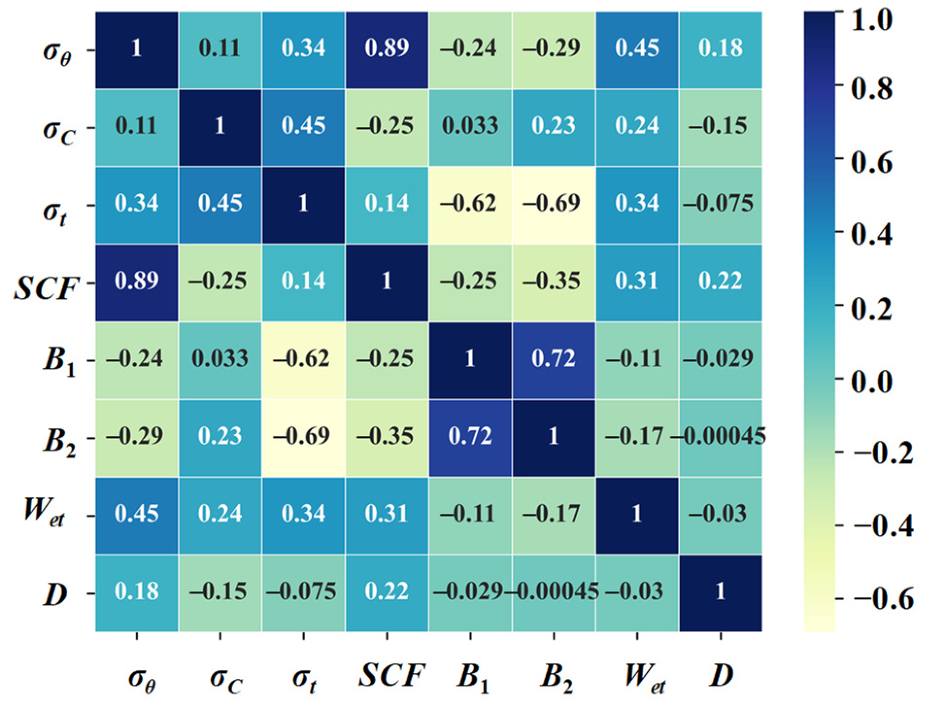
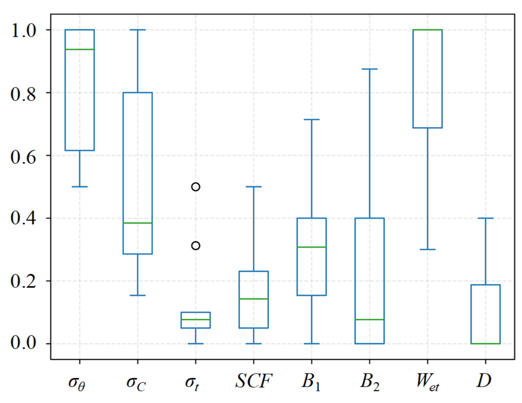
6. Sensitivity Analysis of Features

In order to explore the relative importance of features in rockburst prediction, this paper calculates the contribution rate of each feature to the final prediction accuracy using the Shapley value approach. This is achieved by systematically removing one feature at a time and comparing the prediction accuracy using the incomplete dataset with the accuracy using the complete dataset. The difference between these two results is then used as an index to measure the effect of the specific feature on the prediction accuracy. A larger difference indicates a more important feature in the prediction process.

The change in prediction accuracy for each case of removing one feature at a time is presented in

Table 15. Change in prediction accuracy after removing a corresponding feature from original dataset.

Classifier	σθ	σc	σt	SCF	B1	B2	Wet	D
SVM	0.07	0.01	−0.01	−0.01	0.03	−0.03	0.17	0.02
DT	0.05	0.02	−0.06	−0.03	0	0.03	0	−0.11
LR	0.12	0.2	0.01	0.01	0.02	0.01	0.14	0
KNN	0.09	0.07	0.04	0.01	0.03	0.03	0.02	−0.01
NN	0.17	0.08	0.02	0.02	0.02	0.02	0.18	0.05
Voting method	0.11	0.03	−0.01	−0.02	0.02	−0.02	0.03	−0.02

. This analysis allows us to identify the significance of each feature in the rockburst prediction model and provides valuable insights into their individual contributions.

In Table 15, positive values indicate that the prediction accuracy using the complete database is higher than the accuracy using the incomplete dataset, while negative values suggest that the accuracy of the classifier improves after removing a feature, indicating that the corresponding feature may act as a disturbance variable.

To display the relative importance of features more clearly, the values in each row of Table 15 are normalized to consider the differences between various classifiers. The importance of each feature can then be comprehensively analyzed by considering different classifiers. The statistical results are represented in a box diagram, as shown in Figure 26. This diagram shows that σ_θ, σ_c, and W_et are the first three relatively important features, with W_et having the highest importance, followed by σ_θ and σ_c. On the other hand, B₁, σ_t, SCF, B₂, and D have little influence on the rockburst prediction.

After identifying the critical influencing features (W_et, σ_θ, and σ_c), the distribution of sample points in the corresponding three-dimensional space (W_et-σ_θ-σ_c) is explored to visualize the significance of these key features in predicting rockburst occurrences, as shown in Figure 27. It can be observed that when W_et is large (>5), the grades are basically higher than light rockburst. As for a low level of W_et, the differentiation of rockburst grades can rely on σ_C, as indicated by the approximate layering phenomenon shown in Figure 27. Specifically, no rockburst instances happen when σ_C > 150 MPa. This observation aligns with the common understanding that a higher value of W_et signifies a greater intensity of a rockburst incident, while a higher value of σ_C indicates a stronger capacity of the surrounding rock to withstand external stress.

7. Discussion

Based on the verification results from the database and case validations, the proposed combination model shows promise in predicting strainbursts, which are often encountered in the competent and continuous surrounding rock. However, there are additional features that might influence rockburst occurrences, such as pre-existing fractures or faults in the surrounding rock, as well as tribo-fatigue behavior [59,60,61,62]. These features are not included in the current model due to insufficient data.

This limitation highlights a potential direction for future research. Exploring methods to integrate data concerning pre-existing geological structures and rock behavior as supplementary input variables could enhance the comprehensiveness of our predictive model. By considering these complexities, we could refine our predictions and extend the applicability of the model to a broader range of real-world scenarios.

8. Conclusions

To realize long-term rockburst prediction, a voting ensemble machine learning model was used to establish the non-linear relationship between inducing features (σ_θ, σ_c, σ_t, SCF, B₁, B₂, W_et, and D) and rockburst intensity. A dataset including 344 samples related to rockburst cases was preprocessed by imputing missing feature values and relabeling the dataset. Four optimization algorithms were utilized to search for the optimal hyperparameters of the base learners. Following the performance evaluation, the optimal combination model was selected and applied to two engineering cases for rockburst prediction. The primary conclusions of this study are as follows:

(1)

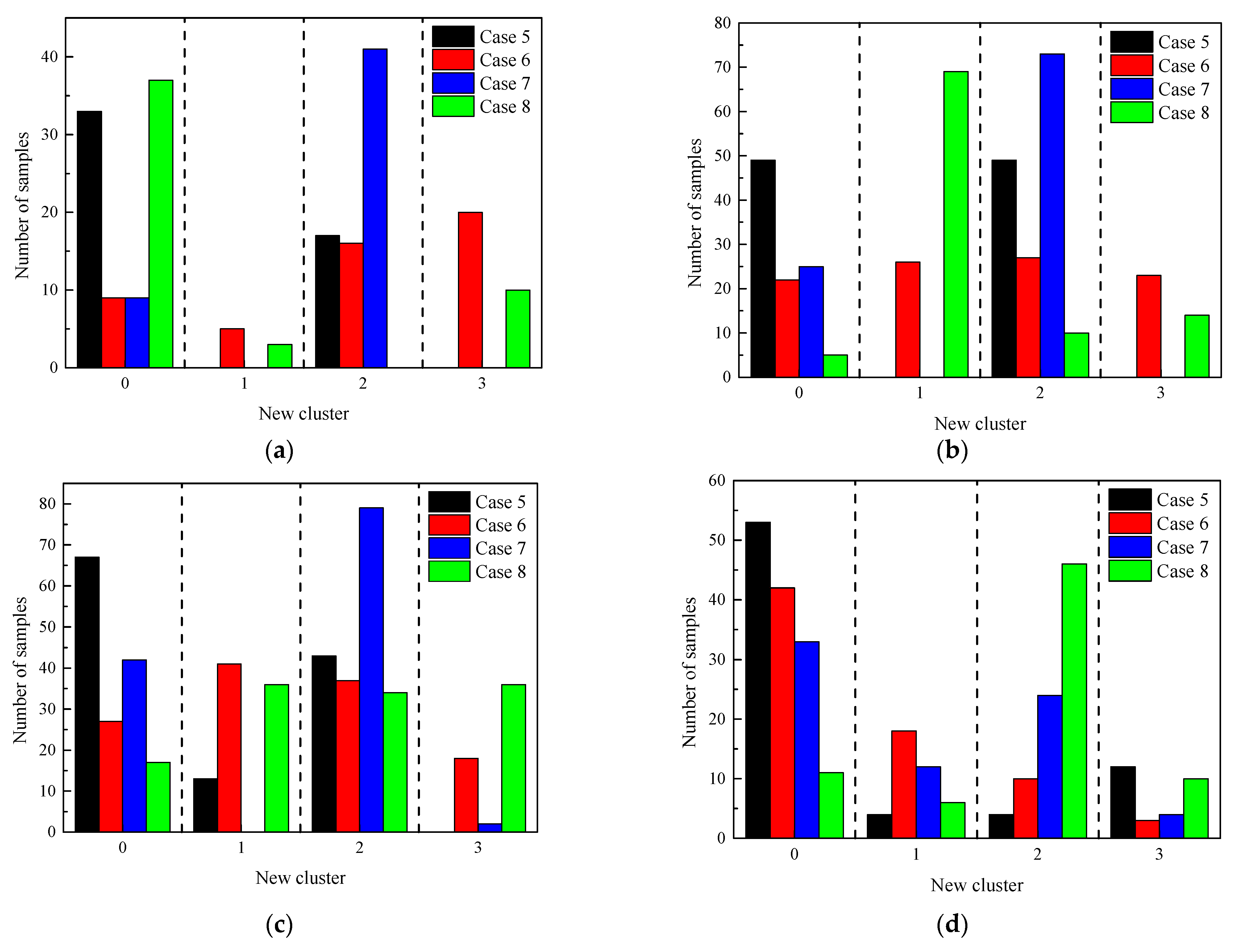
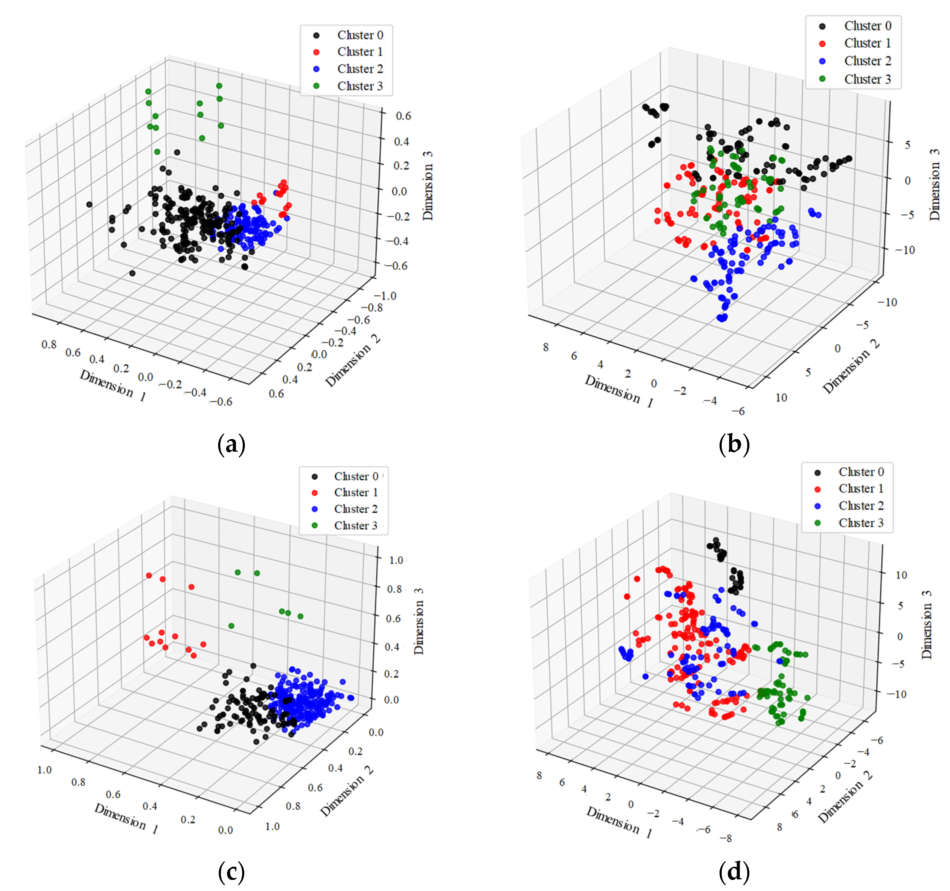
In the process of relabeling the dataset, we used four combination methods (PCA + GMM, PCA + t-SNE + GMM, FS + GMM, and FS + t-SNE + GMM) to reduce the dimensionality of features and perform clustering. It was observed that PCA + t-SNE + GMM and FS + t-SNE + GMM outperformed the other two methods. This is because t-SNE can effectively handle outliers, leading to better clustering results. Moreover, the clustering effect of FS + t-SNE + GMM showed closer agreement with the practical labels compared with PCA + t-SNE + GMM. This is attributed to the susceptibility of PCA to the distribution of sample points and its inability to consider the physical meaning of features. Additionally, the relabeling of the dataset significantly improved both the prediction accuracy of machine learning models and their generalization ability.

(2)

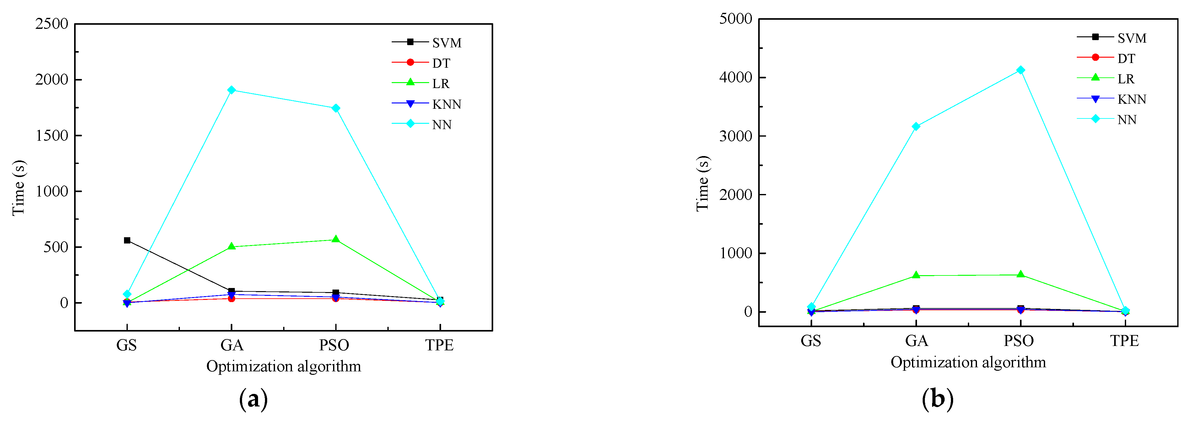
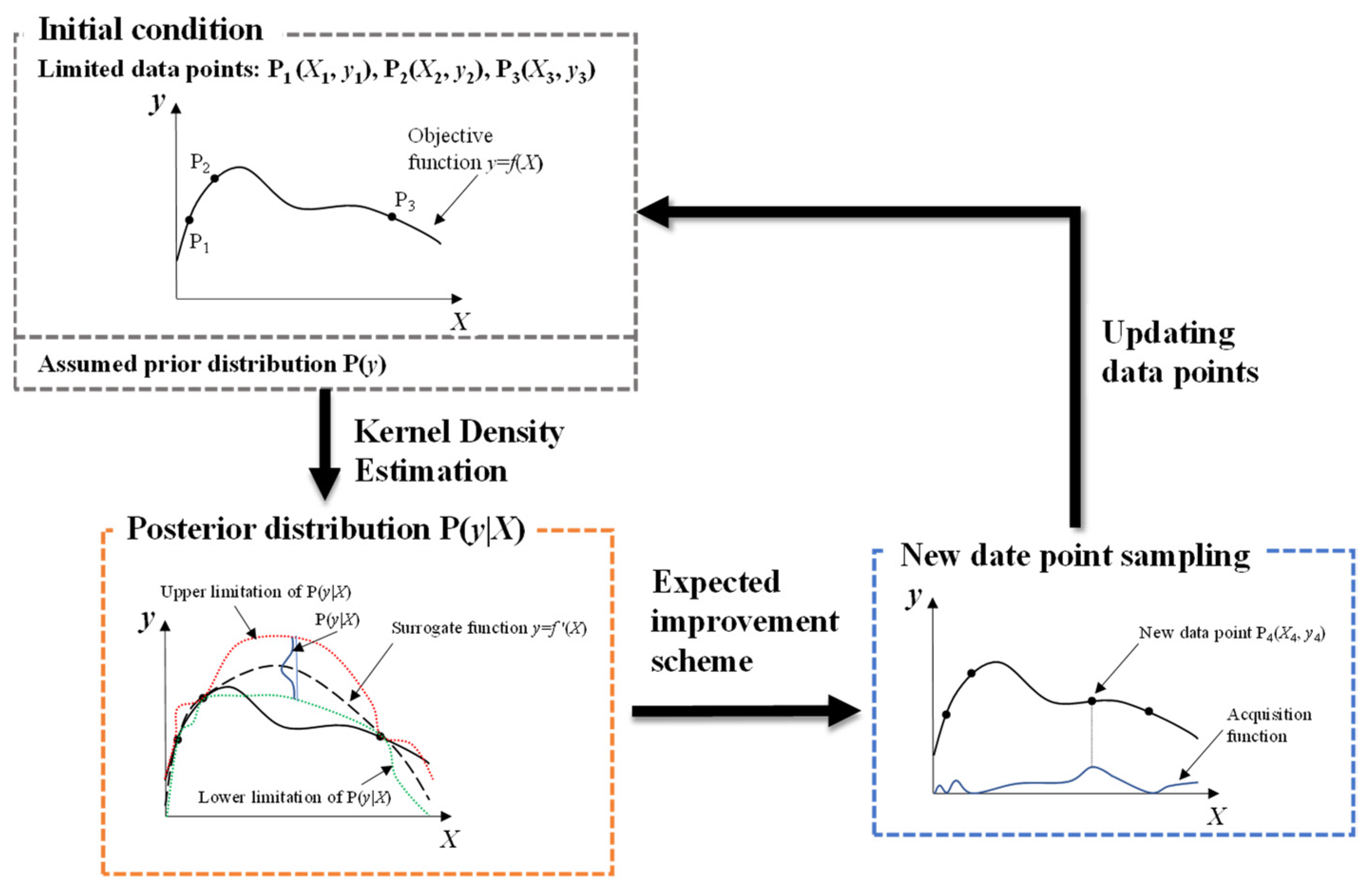
When comparing prevalent hyperparameter optimization algorithms (GS, GA, and PSO), the TPE estimator demonstrated an equal capability in searching for the optimal solution. Notably, TPE’s distinct search strategy, which focuses on the direction of expected improvement, resulted in significant time savings during the optimization process.

(3)

When considering the dataset without preprocessing, the voting ensemble model outperforms the single learners. However, for high-quality datasets, some single learners may exhibit slightly higher precision accuracy compared with the voting ensemble model. Despite this observation, the voting ensemble model consistently achieves satisfactory prediction accuracy by effectively balancing out the weaknesses of individual base learners.

(4)

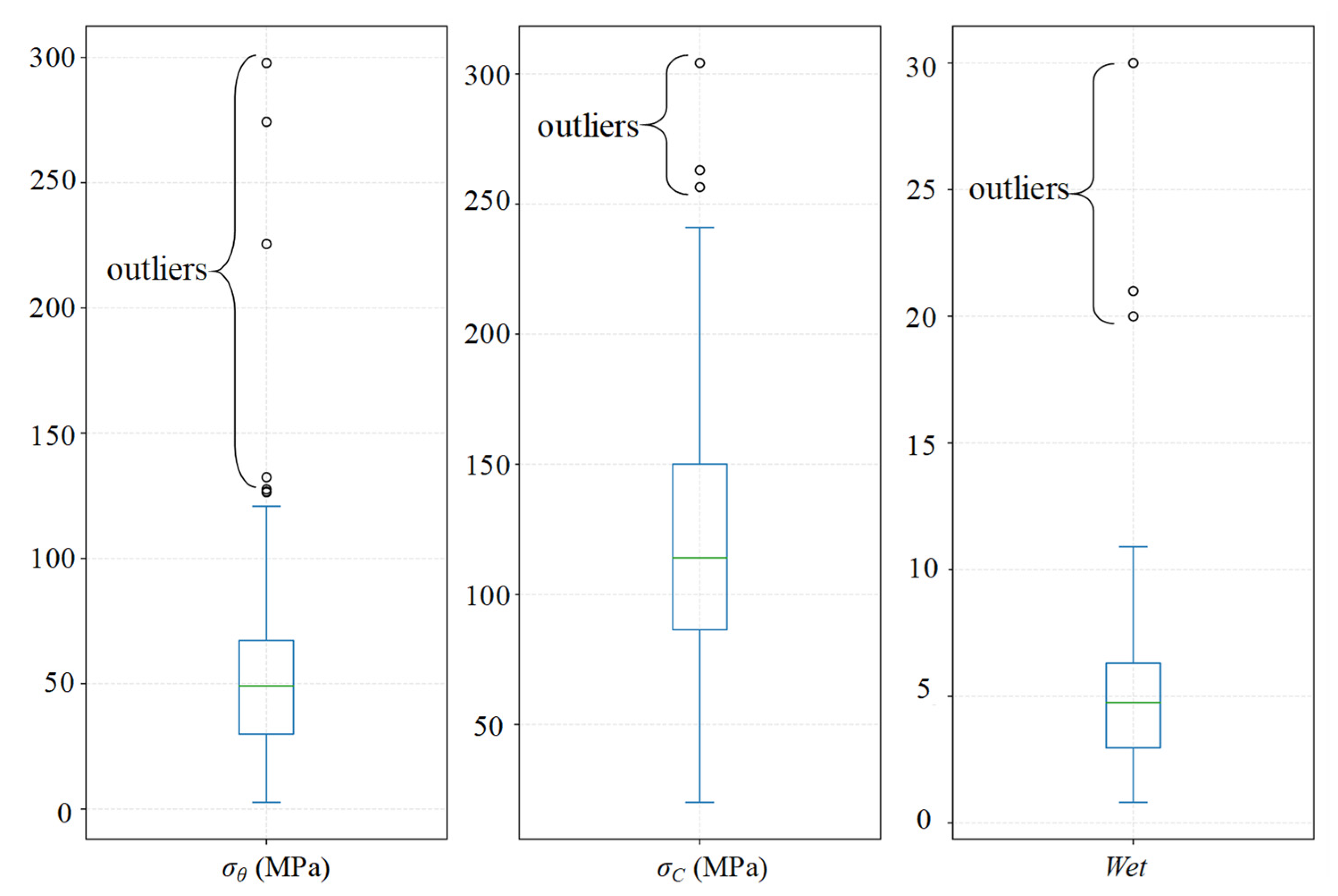
To assess the sensitivity of features to rockburst prediction, we analyzed the contribution rate of each feature. The results indicate that W_et has the most significant impact on rockburst prediction, followed by σ_θ and σ_c. Specifically, a high value (>5) of W_et often indicates a high rockburst intensity, which is typically more severe than a light rockburst. Conversely, a high value (>150 MPa) of σ_c usually implies a lower likelihood of rockburst occurrences. Additionally, light rockbursts and moderate rockbursts often tend to occur when W_et < 5 and σ_c < 150 MPa.

(5)

The proposed combination model was applied to two engineering cases for rockburst prediction. The minor discrepancies between the prediction results and actual rockburst situations underscore the reliability and effectiveness of the model. It is important to note that the proposed model demonstrates particular efficacy in estimating strainbursts. Furthermore, it has the potential to be extended to predict fracture-related rockbursts by incorporating some features related to pre-existing geological structures into the dataset. This presents an avenue for future research and development.

References

1. Wu, S.C.; Wu, Z.G.; Zhang, C.X. Rock burst prediction probability model based on case analysis. Tunn. Undergr. Space Technol. 2019, 93, 103069. [Google Scholar] [CrossRef]
2. Durrheim, R.J. Mitigating the risk of rockbursts in the deep hard rock mines of South Africa: 100 years of re-search. In Extracting the Science: A Century of Mining Research; SME: Southfield, MI, USA, 2010; pp. 156–171. [Google Scholar]
3. Zhang, C.Q.; Feng, X.-T.; Zhou, H.; Qiu, S.L.; Wu, P. Case Histories of Four Extremely Intense Rockbursts in Deep Tunnels. Rock Mech. Rock Eng. 2012, 45, 275–288. [Google Scholar] [CrossRef]
4. Ma, Z.K.; Li, S.; Zhao, X.D. Energy Accumulation Characteristics and Induced Rockburst Mechanism of Roadway Surrounding Rock under Multiple Mining Disturbances: A Case Study. Sustainability 2023, 15, 9595. [Google Scholar] [CrossRef]
5. Pu, Y.Y.; Apel, D.B.; Lingga, B. Rockburst prediction in kimberlite using decision tree with incomplete data. J. Sustain. Min. 2018, 17, 158–165. [Google Scholar] [CrossRef]
6. Frid, V.; Vozoff, K. Electromagnetic radiation induced by mining rock failure. Int. J. Coal Geol. 2005, 64, 57–65. [Google Scholar] [CrossRef]
7. Rasskazov, I.Y.; Migunov, D.S.; Anikin, P.A.; Gladyr’, A.V.; Tereshkin, A.A.; Zhelnin, D.O. New-Generation Portable Geoacoustic Instrument for Rockburst Hazard Assessment. J. Min. Sci. 2015, 51, 614–623. [Google Scholar] [CrossRef]
8. Hudyma, M.; Potvin, Y.H. An Engineering Approach to Seismic Risk Management in Hardrock Mines. Rock Mech. Rock Eng. 2010, 43, 891–906. [Google Scholar] [CrossRef]
9. Mathew, T.J.; Sherly, E.; Alcantud, J.C.R. A multimodal adaptive approach on soft set based diagnostic risk prediction system. J. Intell. Fuzzy Syst. 2018, 34, 1609–1618. [Google Scholar] [CrossRef]
10. Eremenko, A.; Timonin, V.; Bespalko, A.; Karpov, V.; Shtirts, V. Effect of vibro-impact exposure on intensity of geo-dynamic events in rock mass. In Proceedings of the Conference on Geodynamics and Stress State of the Earth’s Interior (GSSEI), Novosibirsk, Russia, 2–6 October 2017. [Google Scholar]
11. Turchaninov, I.A.; Markov, G.A.; Gzovsky, M.V.; Kazikayev, D.M.; Frenze, U.K.; Batugin, S.A.; Chabdarova, U.I. State of stress in the upper part of the Earth’s crust based on direct measurements in mines and on tectonophysical and seis-mological studies. Phys. Earth Planet. Inter. 1972, 6, 229–234. [Google Scholar] [CrossRef]
12. Brown, E.T.; Hoek, E. Underground Excavations in Rock; CRC Press: Boca Raton, FL, USA, 1980. [Google Scholar]
13. Kidybiński, A. Bursting liability indices of coal. Int. J. Rock Mech. Min. Sci. Geomech. Abstr. 1981, 18, 295–304. [Google Scholar] [CrossRef]
14. Aubertin, M.; Gill, D.E.; Simon, R. On the use of the brittleness index modified (BIM) to estimate the post-peak behavior of rocks. In Proceedings of the 1st North American Rock Mechanics Symposium, Austin, TX, USA, 1–3 June 1994; pp. 945–952. [Google Scholar]
15. Gong, F.Q.; Wang, Y.L.; Wang, Z.G.; Pan, J.F.; Luo, S. A new criterion of coal burst proneness based on the residual elastic energy index. Int. J. Min. Sci. Technol. 2021, 31, 553–563. [Google Scholar] [CrossRef]
16. Liang, W.Z.; Zhao, G.Y. A review of research on long-term and short-term rockburst risk evaluation in deep hard rock. Chin. J. Rock Mech. Eng. 2022, 41, 19–39. [Google Scholar]
17. Salamon, M.D.G. Energy considerations in rock mechanics: Fundamental results. J. S. Afr. Inst. Min. Metall. 1984, 84, 233–246. [Google Scholar]
18. Jiang, Q.; Feng, X.-T.; Xiang, T.-B.; Su, G.-S. Rockburst characteristics and numerical simulation based on a new energy index: A case study of a tunnel at 2,500 m depth. Bull. Eng. Geol. Environ. 2010, 69, 381–388. [Google Scholar] [CrossRef]
19. Wiles, T.D. Loading system stiffness-a parameter to evaluate rockburst potential. In Proceedings of the 1st International Seminar on Deep and High Stress Mining, Perth, Australia, 6–8 November 2002. [Google Scholar]
20. Zhang, C.Q.; Zhou, H.; Feng, X.T. An Index for Estimating the Stability of Brittle Surrounding Rock Mass: FAI and its Engineering Application. Rock Mech. Rock Eng. 2011, 44, 401–414. [Google Scholar] [CrossRef]
21. Xu, J.; Jiang, J.D.; Xu, N.; Liu, Q.S.; Gao, Y.F. A new energy index for evaluating the tendency of rockburst and its engineering application. Eng. Geol. 2017, 230, 46–54. [Google Scholar] [CrossRef]
22. Li, F.; Korgesaar, M.; Kujala, P.; Goerlandt, F. Finite element based meta-modeling of ship-ice interaction at shoulder and midship areas for ship performance simulation. Mar. Struct. 2020, 71, 102736. [Google Scholar] [CrossRef]
23. Sun, Q.Y.; Zhang, M.; Zhou, L.; Garme, K.; Burman, M. A machine learning-based method for prediction of ship performance in ice: Part I. ice resistance. Mar. Struct. 2022, 83, 103181. [Google Scholar] [CrossRef]
24. Ma, Y.Z.; Royer, J.J.; Wang, H.; Wang, Y.; Zhang, T. Factorial kriging for multiscale modelling. J. S. Afr. Inst. Min. Metall. 2014, 114, 651–659. [Google Scholar]
25. Nivlet, P.; Fournier, F.; Royer, J.J. A New Nonparametric Discriminant Analysis Algorithm Accounting for Bounded Data Errors. J. Int. Assoc. Math. Geol. 2002, 34, 223–246. [Google Scholar] [CrossRef]
26. Kim, J.-H.; Kim, Y.; Lu, W.J. Prediction of ice resistance for ice-going ships in level ice using artificial neural network technique. Ocean Eng. 2020, 217, 108031. [Google Scholar] [CrossRef]
27. Yin, X.; Liu, Q.; Huang, X.; Pan, Y. Real-time prediction of rockburst intensity using an integrated CNN-Adam-BO algorithm based on microseismic data and its engineering application. Tunn. Undergr. Space Technol. 2021, 117, 104133. [Google Scholar] [CrossRef]
28. Yin, X.; Liu, Q.S.; Pan, Y.C.; Huang, X.; Wu, J.; Wang, X.Y. Strength of Stacking Technique of Ensemble Learning in Rockburst Prediction with Imbalanced Data: Comparison of Eight Single and Ensemble Models. Nat. Resour. Res. 2021, 30, 1795–1815. [Google Scholar] [CrossRef]
29. Xue, Y.G.; Li, G.K.; Li, Z.; Wang, P.; Gong, H.M.; Kong, F.M. Intelligent prediction of rockburst based on Copula-MC oversampling architecture. Bull. Eng. Geol. Environ. 2022, 81, 209. [Google Scholar] [CrossRef]
30. Li, N.; Feng, X.D.; Jimenez, R. Predicting rock burst hazard with incomplete data using Bayesian networks. Tunn. Undergr. Space Technol. 2017, 61, 61–70. [Google Scholar] [CrossRef]
31. Pu, Y.Y.; Apel, D.B.; Xu, H.W. Rockburst prediction in kimberlite with unsupervised learning method and support vector classifier. Tunn. Undergr. Space Technol. 2019, 90, 12–18. [Google Scholar] [CrossRef]
32. Zhou, J.; Li, X.B.; Mitri, H.S. Classification of Rockburst in Underground Projects: Comparison of Ten Supervised Learning Methods. J. Comput. Civ. Eng. 2016, 30. [Google Scholar] [CrossRef]
33. Faradonbeh, R.S.; Taheri, A.; Sousa, L.R.E.R.; Karakus, M. Rockburst assessment in deep geotechnical conditions using true-triaxial tests and data-driven approaches. Int. J. Rock Mech. Min. Sci. 2020, 128, 104279. [Google Scholar] [CrossRef]
34. Guo, D.P.; Chen, H.M.; Tang, L.B.; Chen, Z.X.; Samui, P. Assessment of rockburst risk using multivariate adaptive regression splines and deep forest model. Acta Geotech. 2022, 17, 1183–1205. [Google Scholar] [CrossRef]
35. Liang, W.Z.; Sari, A.; Zhao, G.Y.; McKinnon, S.D.; Wu, H. Short-term rockburst risk prediction using ensemble learning methods. Nat. Hazards 2020, 104, 1923–1946. [Google Scholar] [CrossRef]
36. Zhang, J.F.; Wang, Y.H.; Sun, Y.T.; Li, G.C. Strength of ensemble learning in multiclass classification of rockburst intensity. Int. J. Numer. Anal. Methods Géoméch. 2020, 44, 1833–1853. [Google Scholar] [CrossRef]
37. Cheng, W.-C.; Bai, X.-D.; Sheil, B.B.; Li, G.; Wang, F. Identifying characteristics of pipejacking parameters to assess geological conditions using optimisation algorithm-based support vector machines. Tunn. Undergr. Space Technol. 2020, 106, 103592. [Google Scholar] [CrossRef]
38. Xue, Y.G.; Bai, C.H.; Qiu, D.H.; Kong, F.M.; Li, Z.Q. Predicting rockburst with database using particle swarm optimization and extreme learning machine. Tunn. Undergr. Space Technol. 2020, 98, 103287. [Google Scholar] [CrossRef]
39. Zhang, M.C. Prediction of rockburst hazard based on particle swarm algorithm and neural network. Neural Comput. Appl. 2022, 34, 2649–2659. [Google Scholar] [CrossRef]
40. Sun, Y.T.; Li, G.C.; Zhang, J.F.; Huang, J.D. Rockburst intensity evaluation by a novel systematic and evolved approach: Machine learning booster and application. Bull. Eng. Geol. Environ. 2021, 80, 8385–8395. [Google Scholar] [CrossRef]
41. Van Buuren, S.; Groothuis Oudshoorn, K. mice: Multivariate Imputation by Chained Equations in R. J. Stat. Softw. 2011, 45, 1–67. [Google Scholar] [CrossRef]
42. Russenes, B.F. Analysis of Rock Spalling for Tunnels in Steep Valley Sides. Master’s Thesis, Norwegian Institute of Technology, Trondheim, Norway, 1974. [Google Scholar]
43. Zhou, J.; Li, X.B.; Shi, X.Z. Long-term prediction model of rockburst in underground openings using heuristic algorithms and support vector machines. Saf. Sci. 2012, 50, 629–644. [Google Scholar] [CrossRef]
44. Feng, X.T.; Chen, B.R.; Zhang, C.Q.; Li, S.J.; Wu, S.Y. Mechanism, Warning and Dynamic Control of Rockburst Development Process; Science Press: Beijing, China, 2013. [Google Scholar]
45. Pedregosa, F.; Varoquaux, G.; Gramfort, A.; Michel, V.; Thirion, B.; Grisel, O.; Blondel, M.; Prettenhofer, P.; Weiss, R.; Dubourg, V.; et al. Scikit-learn: Machine Learning in Python. J. Mach. Learn. Res. 2011, 12, 2825–2830. [Google Scholar]
46. Jolliffe, I.T. Principal Component Analysis. In Springer Series in Statistics; Springer: New York, NY, USA, 2002; ISBN 978-0-387-95442-4. [Google Scholar] [CrossRef]
47. Bouwmans, T.; Zahzah, E.H. Robust PCA via Principal Component Pursuit: A review for a comparative evaluation in video surveillance. Comput. Vis. Image Underst. 2014, 122, 22–34. [Google Scholar] [CrossRef]
48. Van der Maaten, L.; Hinton, G. Visualizing Data using, t-SNE. J. Mach. Learn. Res. 2008, 9, 2579–2605. [Google Scholar]
49. Guofei9987. Scikit-opt. 2020. Available online: https://github.com/guofei9987/scikit-opt (accessed on 1 January 2020).
50. Akiba, T.; Sano, S.; Yanase, T.; Ohta, T.; Koyama, M. Optuna: A next-generation hyperparameter optimization framework. In Proceedings of the 25th ACM SIGKDD International Conference on Knowledge Discovery & Data Mining, Anchorage, AK, USA, 4–8 August 2019; pp. 2623–2631. [Google Scholar]
51. Kost, S.; Rheinbach, O.; Schaeben, H. Using logistic regression model selection towards interpretable machine learning in mineral prospectivity modeling. Geochemistry 2021, 81, 125826. [Google Scholar] [CrossRef]
52. Peng, N.; Zhang, Y.; Zhao, Y. A SVM-kNN method for quasar-star classification. Sci. China Phys. Mech. Astron. 2013, 56, 1227–1234. [Google Scholar] [CrossRef]
53. Li, Y.L.; Chen, H.; Lv, M.Q.; Li, Y. Event-based k-nearest neighbors query processing over distributed sensory data using fuzzy sets. Soft Comput. 2019, 23, 483–495. [Google Scholar] [CrossRef]
54. Jiao, S.B.; Geng, B.; Li, Y.X.; Zhang, Q.; Wang, Q. Fluctuation-based reverse dispersion entropy and its applications to signal classification. Appl. Acoust. 2021, 175, 107857. [Google Scholar] [CrossRef]
55. Bergstra, J.; Yamins, D.; Cox, D. Making a science of model search: Hyperparameter optimization in hundreds of dimensions for vision architectures. In Proceedings of the International Conference on Machine Learning, Atlanta, GA, USA, 16–21 June 2013; pp. 115–123. [Google Scholar]
56. Fu, H.L.; Li, J.; Li, G.L.; Chen, J.J.; An, P. Determination of In Situ Stress by Inversion in a Superlong Tunnel Site Based on the Variation Law of Stress—A Case Study. KSCE J. Civ. Eng. 2023, 27, 2637–2653. [Google Scholar] [CrossRef]
57. Meng, W.; He, C.; Zhou, Z.H.; Li, Y.Q.; Chen, Z.Q.; Wu, F.Y.; Kou, H. Application of the ridge regression in the back analysis of a virgin stress field. Bull. Eng. Geol. Environ. 2021, 80, 2215–2235. [Google Scholar] [CrossRef]
58. Brown, E.T.; Hoek, E. Trends in relationships between measured in-situ stresses and depth. Int. J. Rock Mech. Min. Sci. Geomech. Abstr. 1978, 15, 211–215. [Google Scholar] [CrossRef]
59. Shcherbakov, S.S. State of Volumetric Damage of Tribo-Fatigue System. Strength Mater. 2013, 45, 171–178. [Google Scholar] [CrossRef]
60. Sherbakov, S.S.; Zhuravkov, M.A. Interaction of several bodies as applied to solving tribo-fatigue problems. Acta Mech. 2013, 224, 1541–1553. [Google Scholar] [CrossRef]
61. Sosnovskiy, L.A.; Bogdanovich, A.V.; Yelovoy, O.M.; Tyurin, S.A.; Komissarov, V.V.; Sherbakov, S.S. Methods and main results of Tribo-Fatigue tests. Int. J. Fatigue 2014, 66, 207–219. [Google Scholar] [CrossRef]
62. Sosnovskiy, L.A.; Sherbakov, S.S. On the Development of Mechanothermodynamics as a New Branch of Physics. Entropy 2019, 21, 1188. [Google Scholar] [CrossRef]
63. Du, Z.J.; Xu, M.G.; Liu, Z.P.; Wu, X. Laboratory integrated evaluation method for engineering wall rock rock-burst. Gold 2006, 27, 26–30. (In Chinese) [Google Scholar]
64. Jia, Q.J.; Wu, L.; Li, B.; Chen, C.H.; Peng, Y.X. The Comprehensive Prediction Model of Rockburst Tendency in Tunnel Based on Optimized Unascertained Measure Theory. Geotech. Geol. Eng. 2019, 37, 3399–3411. [Google Scholar] [CrossRef]
65. Li, T.Z.; Li, Y.X.; Yang, X.L. Rock burst prediction based on genetic algorithms and extreme learning machine. J. Cent. South Univ. 2017, 24, 2105–2113. [Google Scholar] [CrossRef]
66. Liu, R.; Ye, Y.C.; Hu, N.Y.; Chen, H.; Wang, X.H. Classified prediction model of rockburst using rough sets-normal cloud. Neural Comput. Appl. 2018, 31, 8185–8193. [Google Scholar] [CrossRef]
67. Xue, Y.G.; Zhang, X.L.; Li, S.C.; Qiu, D.H.; Su, M.X.; Li, L.P.; Li, Z.Q.; Tao, Y.F. Analysis of factors influencing tunnel deformation in loess deposits by data mining: A deformation prediction model. Eng. Geol. 2019, 232, 94–103. [Google Scholar] [CrossRef]
Figure 1. The heatmap displays the Pearson correlation coefficient matrix of inducing features regarding rockbursts.
Sustainability 15 13282 g001
Figure 2. The proportion of each class in the dataset.
Sustainability 15 13282 g002
Figure 3. Relabeling samples within each class of the original label based on the empirical proneness index: (a) class 0 of the original label, (b) class 1 of the original label, (c) class 2 of the original label, and (d) class 3 of the original label. (The dashed lines represent the division lines for new different classes).
Sustainability 15 13282 g003
Figure 4. Flow chart showing the process of data relabeling.
Sustainability 15 13282 g004
Figure 5. Schematic diagram showing PCA. (The blue dots represent the sample points, and the two arrows represent the direction of two dimensions).
Sustainability 15 13282 g005
Figure 6. Clustering samples within each class of the original label based on dimensionality reduction and clustering methods: (a) class 0 of the original label, (b) class 1 of the original label, (c) class 2 of the original label, and (d) class 3 of the original label. (The dashed lines represent the division lines for new different clusters).
Sustainability 15 13282 g006
Figure 7. Visualization of clustering results in 3-dimensional space for different methods: (a) clustering result of Case 5, (b) clustering result of Case 6, (c) clustering result of Case 7, and (d) clustering result of Case 8.
Sustainability 15 13282 g007
Figure 8. Box-plot e showing outliers in the data for 3 dominative features.
Sustainability 15 13282 g008
Figure 9. Schematic diagram showing inappropriate PCA application.
Sustainability 15 13282 g009
Figure 10. Flowchart showing the model training and prediction process.
Sustainability 15 13282 g010
Figure 11. The procedure for parameter optimization using TPE.
Sustainability 15 13282 g011
Figure 12. Evolution curves showing the cross-validation mean accuracy during the hyperparameter optimization process: (a) results regarding the dataset with the original label and (b) results regarding the dataset with the new label.
Sustainability 15 13282 g012
Figure 13. Duration of the hyperparameter optimizing process using different algorithms with regard to the original dataset and the relabeling dataset: (a) results regarding the dataset with the original label and (b) results regarding the dataset with the new label.
Sustainability 15 13282 g013
Figure 14. Prediction accuracy for the test set using different base learners combined with optimization algorithms: (a) results regarding the dataset with the original label and (b) results regarding the dataset with the new label.
Sustainability 15 13282 g014
Figure 15. Comparison of prediction accuracy on the training set and test set achieved using different machine learning models: (a) results regarding the dataset with the original label and (b) results regarding the dataset with the new label.
Sustainability 15 13282 g015
Figure 16. F1-score for quantifying the prediction quality of different machine learning models: (a) results regarding the dataset with the original label and (b) results regarding the dataset with new label.
Sustainability 15 13282 g016
Figure 17. ROC for each class obtained using the voting ensemble model: (a) results regarding the dataset with the original label and (b) results regarding the dataset with the new label. (The dashed line is the random guessing line, representing the baseline performance of a model).
Sustainability 15 13282 g017
Figure 18. A longitudinal section of the partial tunnel primarily surrounded by granite rock. (The red line represents the tunnel).
Sustainability 15 13282 g018
Figure 19. Numerical model of the strata in the study area.
Sustainability 15 13282 g019
Figure 20. σθ along the tunnel.
Sustainability 15 13282 g020
Figure 21. Results of rockburst grade along the tunnel estimated using the machine learning model.
Sustainability 15 13282 g021
Figure 22. Actual rockburst situation of the tunnel.
Sustainability 15 13282 g022
Figure 23. Comparison between estimated classes and actual classes regarding the 53 rockburst instances.
Sustainability 15 13282 g023
Figure 24. Location and a rockburst occurrence in the practical engineering case: (a) the general location of Jiangbian Hydropower Station, (b) the layout of the diversion tunnel, and (c) a rockburst instance in the diversion tunnel.
Sustainability 15 13282 g024
Figure 25. Comparison between estimated classes and actual classes regarding the 8 rockburst instances in the diversion tunnel.
Sustainability 15 13282 g025
Figure 26. Statistical results showing the relative importance of features by box-plot.
Sustainability 15 13282 g026
Figure 27. Distribution of sample points regarding different classes in Wet-σθ-σc space.
Sustainability 15 13282 g027