Article

A Regional Road Network Capacity Estimation Model for Mountainous Cities Based on Auxiliary Map

1
College of Traffic & Transportation, Chongqing Jiaotong University, Chongqing 400074, China
2
College of Smart City, Chongqing Jiaotong University, Chongqing 400074, China
3
Chongqing Linggu Transportation Technology Co., Ltd., Chongqing 400064, China
*
Author to whom correspondence should be addressed.
Sustainability 2023, 15(14), 11439; https://doi.org/10.3390/su151411439
Submission received: 26 April 2023 / Revised: 4 July 2023 / Accepted: 20 July 2023 / Published: 24 July 2023

Abstract

:
The focus of sustainable urban transportation development lies in realizing the untapped capacity potential of the existing road network and enhancing its operational efficiency without expanding its physical footprint. To quantify the supply capacity of road networks in mountainous cities, this paper converts the problem of solving the capacity of road networks into the problem of solving the minimum cut set in road networks from the perspective of road network capacity, using the idea of the auxiliary diagram method in graph theory. By improving the limitation that the auxiliary map method is only applicable to the single starting point and terminal point network, a regional road network capacity estimation model of a mountain city based on the auxiliary map is constructed. Combined with the actual regional road network, the model results presented in this paper show that the road network capacity calculated by the auxiliary graph method is 30,137 pcu/h. Using the improved traffic distribution simulation method, the network capacity is 38,776 pcu/h. Compared with the traffic distribution simulation method, the regional road network capacity model based on an auxiliary map proposed in this paper is more realistic.

1. Introduction

The planning, construction, and management of urban regional road networks must adhere to a strategic approach to sustainable development. Sustainable urban transport development focuses on realizing the untapped capacity potential of the existing road network and improving its operational efficiency without expanding its physical footprint. The goal is to maximize the functionality of the network while minimizing negative impacts. This approach first requires capturing the existing road network capacity levels. Once the road network capacity in an urban area is insufficient, it can lead to traffic congestion problems that affect mobility and efficiency. Traffic congestion can increase commuting time, energy consumption, and environmental pollution and negatively affect the economic vitality of cities and the quality of life of their residents. An inadequate capacity of the regional road network can lead to outward urban sprawl, which can take up large amounts of agricultural land and natural resources and increase the need for infrastructure construction and maintenance. A high-capacity road network can facilitate the movement of goods and services, improve the economic competitiveness of cities, and help achieve compact urban planning and efficient use of land resources [1]. By providing efficient goods transportation and logistics services, cities are able to attract investment, expand business activities, and provide more employment opportunities. In addition, the capacity of the regional road network is relevant to the development of urban public transportation systems [2,3]. Public transportation is an important component of sustainable urban transport, and by providing convenient, economical, and environmentally friendly travel options, it can reduce reliance on the private automobile, reduce traffic congestion, lower vehicle emissions, improve air quality, and positively impact the urban environment and the health of residents. Therefore, a quantitative study of the capacity of urban regional road networks is necessary to achieve the long-term sustainable development of transportation systems.
The road network layout of mountainous cities is complex, as the land is typically divided into multiple clusters of a specific scale by mountains and rivers, and cities are typically constructed between large mountainous regions with undulating topography and poor road conditions. It is difficult to control the traffic in the main locations scattered throughout the clusters. The prerequisite for the sustainable development of traffic in mountainous cities is to grasp the capacity level of each regional road network, firstly, to strengthen traffic control means on the existing regional road network capacity level and, secondly, to propose measures to improve the regional road network capacity in response to the bottlenecks of the road network. Therefore, this paper focuses on the research of regional road network capacity in mountain cities, quantitatively analyses the supply capacity of the existing regional road network, and provides theoretical support for the sustainable development of transportation in supporting mountain cities.
In this study, an auxiliary-map-based model for estimating the capacity of regional road networks in mountainous cities was constructed to reflect the actual supply capacity of the road network more accurately in mountainous cities. We calibrated the actual road capacity by combining the factors influencing the regional road network capacity, and the minimum cut set in the road network was mined by constructing an auxiliary map of the regional road network to obtain the regional road network capacity of mountainous cities. The main contributions of this paper are as follows:
(1)
This study focuses on the specific characteristics of regional road networks in mountain cities and proposes a definition for the capacity of such networks. The definition takes into account the unique challenges and requirements of road networks in mountainous regions.
(2)
To solve the problem of determining the capacity of regional road networks, the authors utilize an auxiliary graph. This transformation allows them to reframe the problem as finding the minimum cut set of the regional road network. By doing so, they simplify the analysis and calculation process.
(3)
In order to address the limitation of the cut-set method in solving the minimum-cut problem under multiple origin–destination (OD) pairs, the authors propose an improved method for estimating road network capacity in the central business district (CBD) region of mountain cities. The improvements involve adding dummy vertices on each side of the auxiliary graph. These dummy vertices help divide the traffic groups into two separate groups, with each group connected to one of the dummy vertices. This abstraction allows the multiple groups of OD pairs in the regional road network to be treated as a network with a single starting and ending point. The capacity of the road network is then determined using the cut-set method. By employing this approach, the improved method in this study avoids the problem of overlapping in the abstract road network.
The remainder of this paper is organized as follows. Section 2 is a literature review. Section 3 defines road network capacity in mountainous cities. In Section 4, we describe the construction of a capacity model of the road network. In Section 5, the application of the proposed model is verified. Finally, Section 6 presents the conclusions and prospects of the study.

2. Literature Review

Currently, models and methods for calculating road network capacity include the cut-set method, the traffic distribution simulation method, the space–time consumption method, and linear programming. As early as 1956, Ford [4] and Beckmann [5] proposed the network maximum-flow problem for calculating road network capacity based on capacity, and the cut-set method was used to analyze road traffic problems. The main idea of the cut-set method is to use the maximum-flow minimum-cut theorem to calculate road network capacity, which more accurately reflects the intrinsic relationship between the physical structure of road networks and traffic demand. Subsequently, Masuya [6] utilized network flow cut-set theory to determine the capacity of a road network. Martha [7] evaluated the impact of two-way road medians, investigated the adjustment factor for road capacity calculation based on the median type, and validated the results. Ramesh [8] used the distributed Edmonds–Karp algorithm to improve the cut-set method and apply it to large urban networks, and the model can effectively improve the safety of large urban road networks. Wei et al. [9] conducted qualitative and quantitative research on the road network capacity of Beijing. Mikulai et al. [10] proposed a model to objectively identify the weak points of the road infrastructure in the Western Hungarian region, a typical part of the Hungarian road network, based on automated data input.
Asakura et al. [11] proposed a traffic assignment simulation approach that employed traffic assignment to discover the cut set of a road network. This method was used by Iida [12] to determine the maximum capacity of a road network. The traffic assignment simulation method was then used by Baskan [13] and Zhang [14] to undertake an in-depth study of road network capacity expansion. Vincenza [15] recognized that road network capacity is a crucial measure for traffic planning and management; thus, he used the real-time simulation results of the dynamic traffic assignment model to calculate it. Several aspects of the traffic flow relationship in large-scale, complicated urban street networks were investigated. Later, Jiang et al. [16] used the traffic assignment simulation method to calculate road network capacity while accounting for the effects of parking supply and parking prices to evaluate urban road network capacity. Zhou et al. [17] developed a two-tier planning model for hybrid traffic flow assignment and proposed to save the time cost of travel by increasing the market penetration of driverless cars. This calculation method is simple and practical and can identify key sections of the road network. Zhang et al. [18] presented a new model to calculate the maximum equilibrium road network capacity and obtain the associated optimal origin–destination (i.e., OD) flow pattern for a general road network with the given network topology and link attributes. Anupriya et al. [19] estimated macroscopic fundamental relationships for homogeneously congested sub-networks (reservoirs) in thirty-four cities worldwide. The purpose of Pospelov et al. [20] was to clarify the traffic flow composition and determine the passenger car equivalent coefficients in modern traffic conditions.
The spatio-temporal consumption method was first proposed by the French engineer Louis Marchand, who assigned spatio-temporal properties to the road network. The algorithm is simple but considers more parameters. Zhang et al. [21] developed a road network capacity model based on the spatio-temporal consumption method for assessing the reliability of road network capacity. Liu et al. [22] used this method to evaluate the effects of car sharing on traffic congestion management by analyzing the changes in travel time and space consumption caused by car sharing. Mo and Shao et al. [23,24] developed a spatial-temporal consumption enhancement model based on road structure and classification. Xu et al. [25] constructed a road network capacity model based on road classification by considering the efficiency differences between different classes of roads in cities based on the spatio-temporal consumption method. Although the spatio-temporal consumption method is straightforward and simple to comprehend, the calibration and calculation of the parameters for the correct result are challenging.
Wong [26] applied the notion of road network capacity to the problem of traffic signal management and utilized a two-level planning model to determine the maximum carrying capacity of a traffic network under traffic signal control. Masuya [27] devised and verified a linear programming approach based on the cut-set method. The linear programming method is conceptually identical to the cut-set method, but its computational effort is enormous. Ji et al. [28] created a reliability analysis algorithm based on the SUE model to optimize a two-level planning model for road network capacity. Wang [29] and Yang [30] created a corresponding two-level planning model for road network capacity, considering the level of service constraints and the spread of road congestion. Conlan et al. [31] studied the problem of collectively processing shortest path queries, where the objective is to optimize a collective objective, such as minimizing the overall cost.
Combining the existing research results, a comparison of the cut-set method, the traffic distribution simulation method, the space–time consumption method, and the linear programming method is shown in Table 1.
The majority of research on road network capacity is still theoretical, and there is a dearth of research that combines theoretical models with actual road networks. Simultaneously, the study of the theoretical model is imperfect, the form of the theoretical model is complex and difficult to compute, the model’s parameters are numerous and difficult to calibrate precisely, and the model’s accuracy and applicability are low. The following issues are prevalent at present:
(1)
The linear programming approach considers many influencing elements, but the data involved are difficult to extract and effectively analyze, and the model form is complex, making it difficult to find an exact solution to the road network’s capacity.
(2)
The spatio-temporal consumption method cannot accurately reflect the real traffic demand distribution of the city, and the road network capacity calculated by the spatio-temporal consumption model is generally higher than the actual road network capacity of the city. There are more parameters in the model, and the extraction of the basic data required by the model is frequently labor-intensive and impractical.
(3)
Owing to the vast variance in road traffic systems between cities, it is impossible to create a consistent model for calculating the road network capacity of every city.

3. Definition of Road Network Capacity in Mountainous Urban Areas Based on Cut-Set Method

To solve the road network capacity problem, the cutting-set approach is primarily based on the maximum-flow and minimal-cut theorem.
Ford [4] created the 2F algorithm, which starts with a feasible flow in the network, identifies an augmentation chain from the origin point to the receiving point, adds new traffic, and generates a new viable flow. The flow is then increased by finding an augmentation chain between the originating site and the receiving location. This process is repeated until no augmentation chains are located in the road network, at which point the flow is maximum. The 2F algorithm, on the other hand, is only relevant to networks with a single starting and ending point and a specified direction, and it is inapplicable to networks with random starting and ending points and no fixed direction.
To address the shortcomings of the 2F algorithm, the derived cut-set network extreme flow (ECS) algorithm has also been proposed. The principle of the ECS algorithm is that after giving the initial set of originating and receiving points for finding the minimum cut set in the road network, the derived source set is gradually expanded starting from the originating set, and the edges between the derived source set and the set of neighboring points of the derived source set form a new cut set. In the process of gradually expanding the derived source set, each intermediate point on the network is successively transformed from an originating point to a receiving point until the last receiving point set. However, the ECS algorithm also has a shortcoming in that the number of cut sets of a network usually grows exponentially with an increase in the number of derived points, and when there are many derived points in a network, the number of cut sets is also very large, which is not suitable for solving complex urban road network congestion problems.
The auxiliary diagram algorithm’s principle is to abstract the example road network into a simplified network connected by points and lines and then construct the auxiliary diagram of the original diagram on the simplified network with certain principles, using Floyd and other algorithms to find the shortest cut in the auxiliary diagram. Because the shortest circuit and minimum cut have duality, finding the shortest circuit in the auxiliary graph corresponds to finding the smallest set of cuts in the actual road network. The constructive auxiliary graph algorithm has the limitation that it is applicable only to one-way network problems with a single origin and destination.
According to the above analysis, most existing approaches are still theoretical, with issues such as extensive calculations and unsuitability for application in the study of urban road networks, making it impossible to tackle practical traffic problems. As a result, this study proposes a definition of road network capacity in hilly urban regions based on the cut-set method: the total number of vehicles that can pass through the minimal cut set in the road network per unit of time, given particular road conditions and traffic regulations. Road network capacity is defined as the sum of the capacity of the road sections formed by the minimum cut set proposed in the cut-set approach.
In terms of the definition of the actual capacity of the regional road network, it is still worth noting the following:
(1)
Road network capacity refers to the maximum traffic flow that the road system can carry in a specific period of time. Different sections of the regional road network have different capacity levels affected by road conditions. Therefore, critical sections will determine regional road network capacity.
(2)
Capacity is a reference flow, which is considered valid for a period of one hour but usually is computed using data from shorter periods of 15 min or less.
(3)
Any figure on capacity is not indicating an absolute maximum, but rather a reference value to which the flow will tend. Thus, it is possible to observe a particular flow of vehicles/hour that is above the theoretical maximum capacity.

4. Methodology

4.1. Model Construction Ideas

According to the cut-set method’s definition of road network capacity in hilly urban regions, the total capacity of road sections formed by the minimal cut set proposed in the cut-set method can be described as the road network capacity. As a result, the fundamental challenge of applying the cut-set method to solve road network capacity in mountainous metropolitan regions is to determine the lowest cut set in the road network.
The theory behind using the auxiliary diagram approach to solve the minimal cut set and road network capacity of the road network in mountainous urban areas is as follows in Figure 1.
Step 1: Create a basic abstract road network G based on actual road network maps of mountainous urban areas. The capacity is corrected based on the key influencing variables of the road network capacity of mountainous urban areas and the capacity of each road segment in the road network G .
Step 2: Build the auxiliary map road network G on top of the initial road network G * .
Step 3: Use computer programming procedures to identify the shortest path in G * .
Step 4: Print the road segment in G corresponding to the shortest circuit in G * , which is the minimal cut set.
Step 5: The sum of the capacity of the road sections corresponding to the minimum cut set is the capacity of the road network in the mountainous urban area.

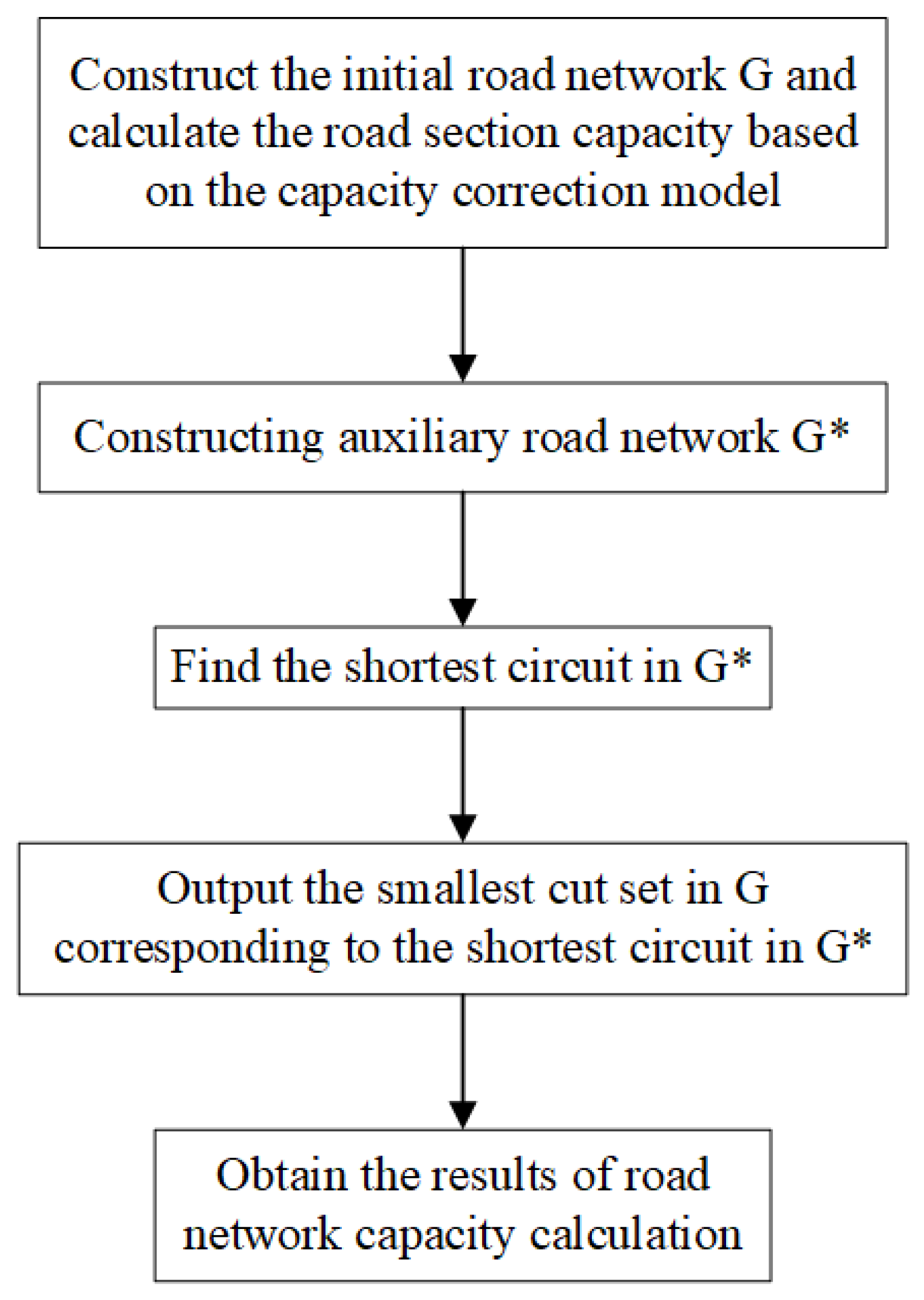
4.2. Auxiliary Diagram Shortest-Circuit Model

Define a network G = { V , E , C } . According to cut-set theory, it is known that V is the set of points of G , E is the set of arcs of G , and C is the right of the network. The edges of G dissect the plane into several regions, each of which is called the face of G . One of the faces is unbounded and is called the outside, and the other is called the inside. For a network G , it is always possible to draw v s on the left side of the network G and v t on the right side of the network G . Suppose there are two vertical lines that pass through points v s and v t , at which point the outside becomes four parts, calling the part above G the top and the part below G the bottom. As shown in
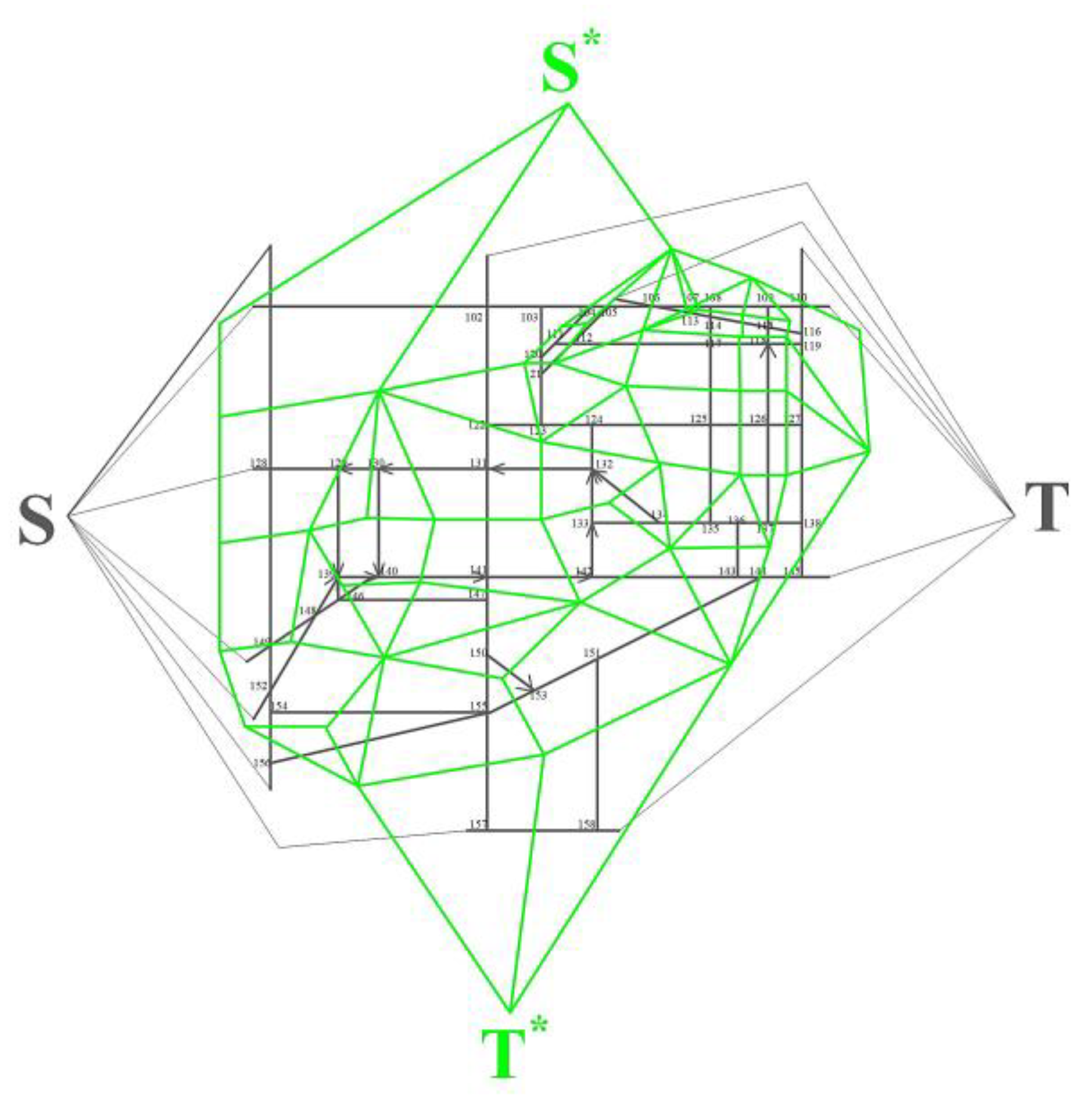
 Figure 2, F 1 is the top of G , F 2 and F 3 are the inner part of G , and F 4 is the bottom of G .
Suppose there exists a subset X of V satisfying x X and y X ¯ = V X . The following set can be defined.
Φ X = uv u X , v X ¯   o r   u X ¯ , v X
O X = uv u X , v X ¯
I X = uv u X ¯ , v X
O ( X ) is the cut set of G . Equation (4) is called the capacity of the cut set O ( X ) .
C ( O ( X ) ) = ε O ( X ) C ( e )
When two adjacent edges in the sequence e i 1 , e i 1 e i k of edges are at the boundary of the same side, the sequence is a set of edges in the network G . Two e 1 and e 2 in Φ ( X ) are said to be connected to Φ ( X ) if e i 1 = e 1 and e i k = e 2 .
When two edges in the set commute with Φ ( X ) , the set is said to commute with Φ ( X ) . Also, the following theorem follows: if O ( X ) is a minimal cut set, then any two edges in O ( X ) are commutative with Φ ( X ) .
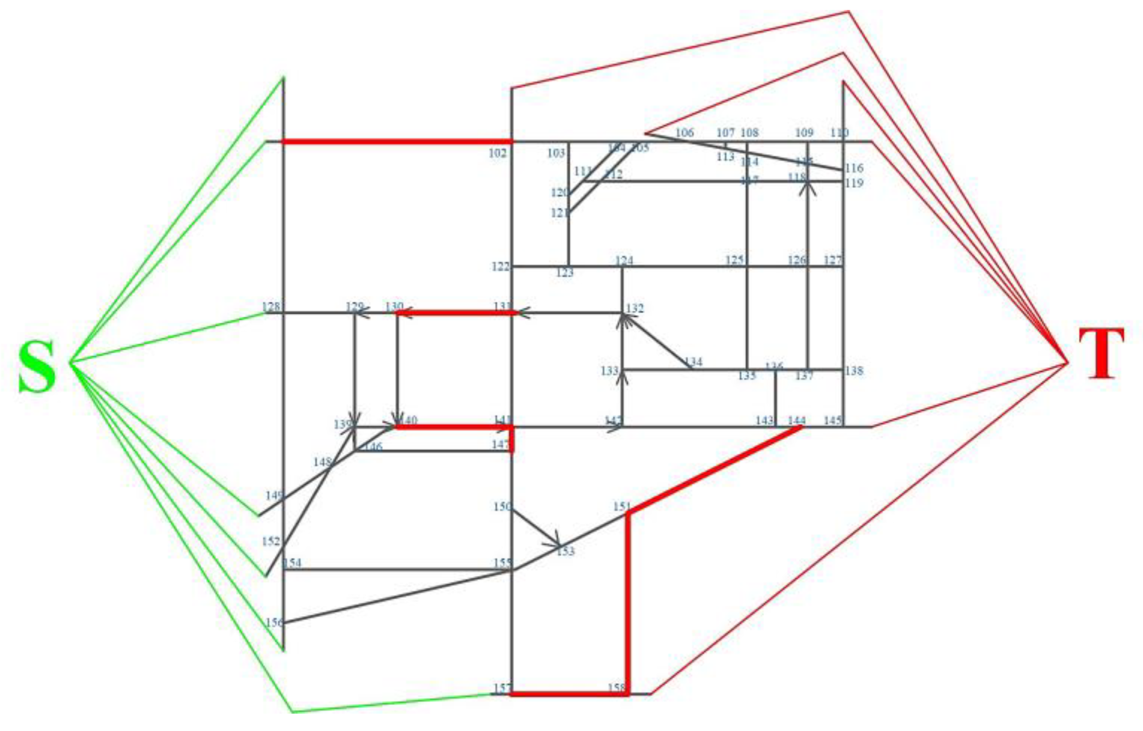
Because the shortest cut has duality with the minimum cut, the minimum cut set of the network G can be obtained by finding the shortest cut between its auxiliary graph G * and the sending point v s * to the receiving point v t * .
The auxiliary graph G * is constructed as follows: each inner face F in G has a vertex v * of G * corresponding to it, the top of G has a vertex v s * of G * corresponding to it, and the bottom of G has a vertex v t * of G * corresponding to it. When the faces in G are adjacent, the vertices in the G * are also adjacent. Each pair of adjacent vertices of G * has a pair of directed edges with opposite directions between them, and its right is defined by the following method: let v i * and v j * correspond to the faces of G * , there exist directed edges v i * v j * and v j * v i * , v i * and v j * correspond to the faces of G denoted as F i and F j , respectively, the common boundary of F i and F j is denoted as l i j , and l i j is a chain. If G* is drawn on G, v i * can be drawn on F i and v j * in F j . The pointing of v i * v j * , when v i * v j * coincides with l i j is called the l i j ’s by v i * v j * the direction determined by v i * v j * . Therefore, it is also obtained that the direction of l i j is determined by the direction of v j * v i * , and the two directions of l i j are opposite. The formula is as follows.
l i 0 = { e | e l i j , and the direction is the same as that determined by v i * v j * } .
l 0 j = { e | e l i j and in the direction opposite to the direction determined by v i * v j * } .
Specify the right on the edge v i * v j * as
W ( v i * v j * ) = 0 min C ( e ) e l i 0 l 0 j Φ l 0 j = Φ
If l 0 j Φ , the right W ( v i * v j * ) corresponds to the set of edges l 0 j . If l 0 j = Φ , the right W ( v i * v j * ) is said to correspond to the set of edges l i 0 = { e | e l i 0 and C ( e ) = W ( v i * v j * ) } , similarly defining W ( v j * v i * ) .
For a vertex v i * adjacent to v s * , only the directed edge v s * v i * and the weight W ( v s * v j * ) on it need to be defined; for a vertex v j * , adjacent to v t * , only the directed edge v j * v t * and the weight W ( v i * v j * ) on it need to be defined.
When computing the shortest path from v s * to v t * in the G length of a path P is the sum of the weights on its upper edges, denoted by W ( P ) , which is expressed as follows:
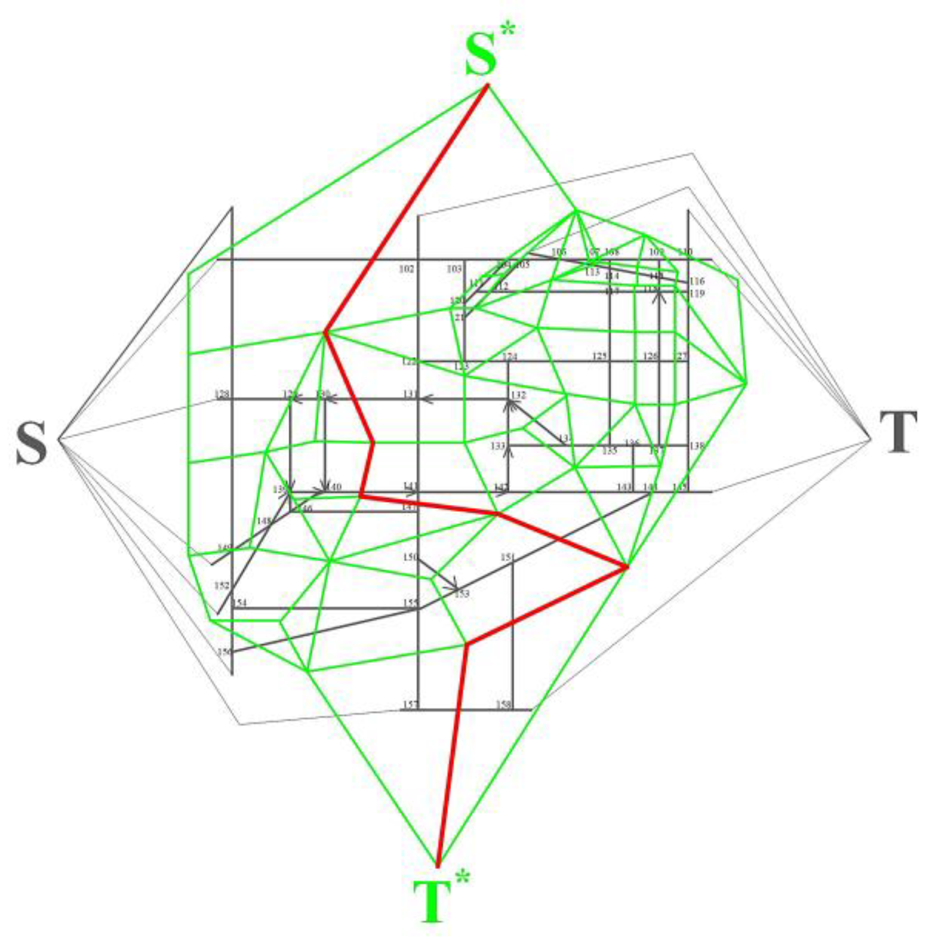
W ( P ) = e P W ( e )  
The auxiliary graph G * of the network G is shown in Figure 3.
It can be seen that the auxiliary graph G * is constructed so that v i * v j * always intersects the edges in the corresponding Φ ( X ) in G , and their powers correspond to each other. v s * to v t * also divides the vertices of G into two parts, and the shortest cut in the auxiliary graph G * corresponds to the smallest cut in the network G . The shortest cut in the auxiliary graph G * corresponds to the shortest cut in the network G . Therefore, when all the shortest paths in the auxiliary graph G * are found, the set of minimal cuts in G is obtained based on the fact that the edges in the auxiliary graph G * correspond to the edges in the network G .
The approach is relevant in the following situations:
(1)
Planar road network: This means that the network can be simplified to a road network in which the edges only interact at the vertices.
(2)
A one-way road network with a single start and finish point: The network is typically multi-start and undirected, and therefore, the approach must be improved.
The auxiliary graph shortest-circuit algorithm was improved as follows:
(1)
The road network abstraction is simplified into a directionless network.
Most of the roads in the urban road network are bidirectional; therefore, we simplify the road network into an undirected network.
(2)
Determine the set of sending and receiving points.
The feasible flows of undirected graphs are typically reflected in multiple logistics with multiple sending and receiving points. For the flow problem of deterministic networks, the set of sending and receiving points in the network must be determined.
(3)
Add two dummy vertices v s and v t to the network and connect each node in the set of sending and receiving points to the two dummy vertices, respectively. To ensure that the changed network is consistent with the actual network capacity, the capacity between v s and all sending points and the capacity between all receiving points and v t are set to infinity.
The main process of solving the capacity of the road network using this algorithm is to construct the undirected auxiliary road network G * from the undirected road network G , find the shortest path in G * , and then determine the smallest cut set in G . The sum of the capacity of the smallest cut set in G is the capacity of the road network.
Combining the above studies, the construction of the auxiliary graph G * can be obtained as follows: for each inner face F of G , there is a vertex v * of G * corresponding to it; for the top of G , there is a vertex v s * of G * corresponding to it; for G below, there is a vertex v t * of G * corresponding to it; and the right of each side of G * is equal to the right of the corresponding edge in G that intersects it. All edge weights of G * are obtained from the edge weights in G , which commute about Φ ( X ) .

4.3. Construction of Road Network Capacity Estimation Model for Mountainous Urban Areas Based on Auxiliary Map Method

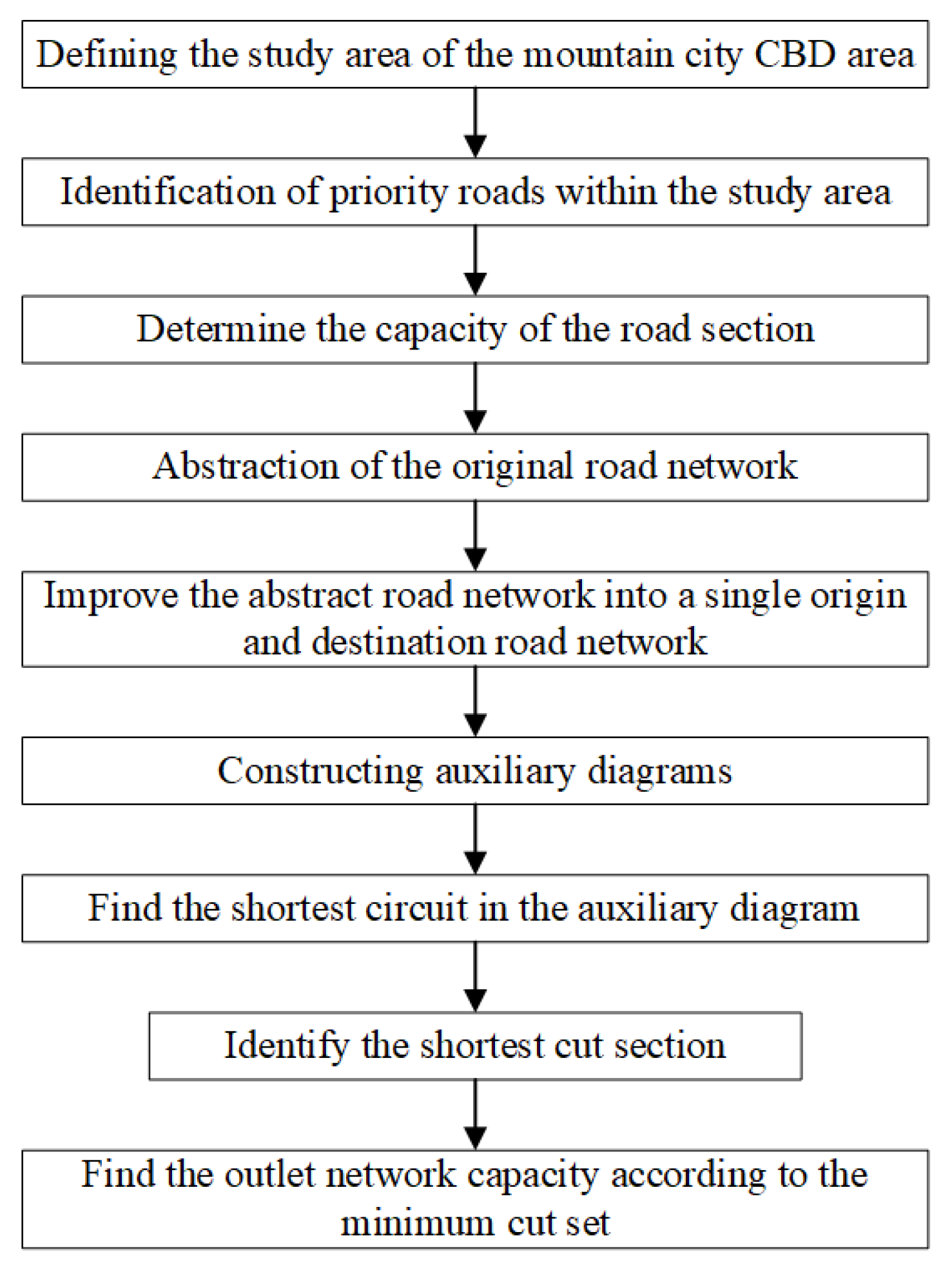
Based on the above analysis, the main process for constructing a road network capacity estimation model for mountainous urban areas based on auxiliary maps is as follows:
(1)
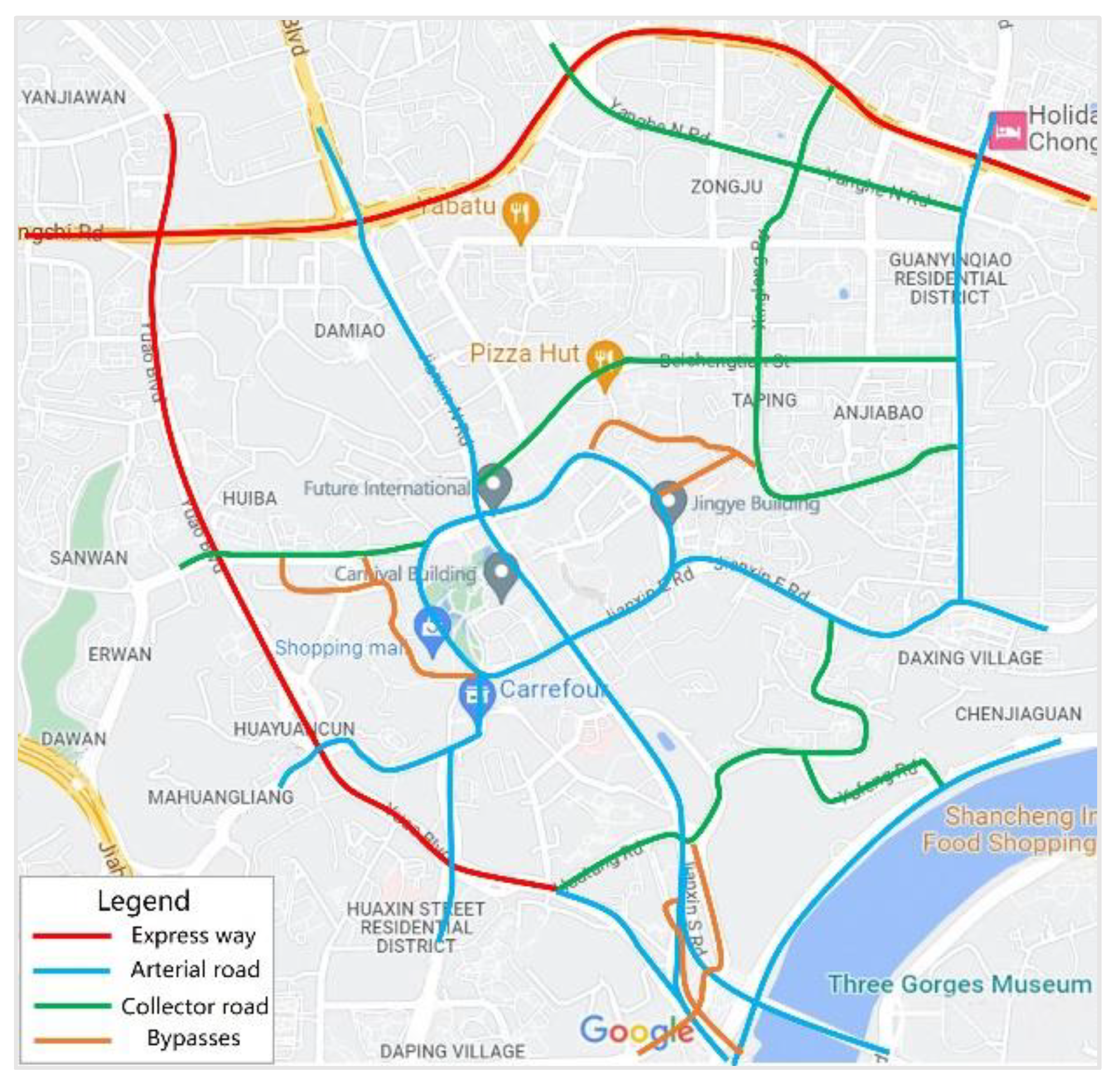
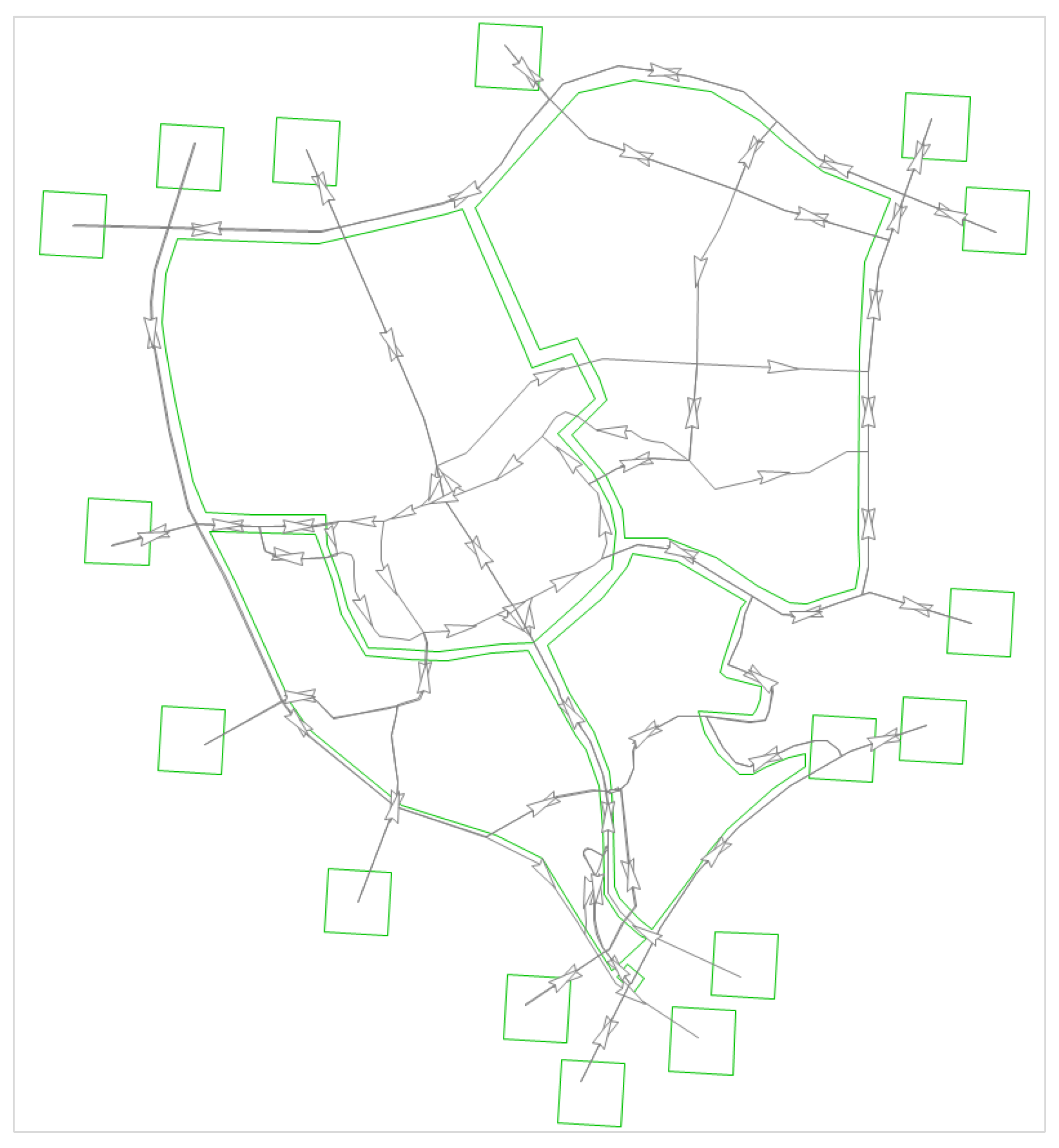
Determining the study area as a mountainous urban area
The study area is typically the area enclosed by expressways or trunk roads around the business district.
(2)
Determining the key roads in the study area
Throughout the study area, expressways, principal and minor highways, and feeder roads are investigated. Among them, “part of the branch road” refers to the study of a branch road if both ends are connected with secondary roads and above, and it serves as a traffic converter between secondary roads and above.
(3)
Determining the capacity of the road section
According to the problems studied in this paper, it is known that the right of each road section should take the capacity of the road section. However, because of the mountainous urban area road network in the layout structure, function, and grade structure compared with the plain city, there are obvious characteristics that should be specifically studied in the mountainous urban area road network in the section of the capacity. The capacity of road sections in hilly cities’ regional road networks should be assessed as follows.
(4)
Abstraction of original road network
The road network is abstracted. According to the abstraction principle of graph theory, intersections are abstracted as nodes, and the road sections are abstracted as arcs connecting the nodes.
(5)
Transforming the abstract road network into a single origin and destination road network
All the “originating points” will be gathered to the originating point S , and all the “receiving points” will be gathered at the receiving point T .
(6)
Construction of an auxiliary diagram
In the abstracted single origin and destination road network diagram, an auxiliary diagram is constructed according to the construction method of the auxiliary diagram.
(7)
Determining the shortest circuit in the auxiliary diagram
Computer programming can be used to find the shortest circuit in the auxiliary diagram, the shortest circuit of all sections cut, and the minimum set of cuts in the road network. In this paper, Floyd’s algorithm is used to determine the shortest circuit in the auxiliary diagram.
(8)
Finding the shortest cut section
Floyd’s algorithm is used to find the actual road section corresponding to the shortest cut in the auxiliary diagram, i.e., the minimum set of cuts in the road network.
(9)
Finding the capacity of the road network according to the minimum cut set
After determining the minimum cut set in the road network, the capacity of the road sections corresponding to the minimum cut set is summed to obtain the capacity estimation result of the road network in mountainous urban areas based on the auxiliary map method.
The process of using the auxiliary diagram method to determine the capacity of the road network in mountainous urban areas is shown in Figure 4.

4.4. Modified Model for Road Capacity in Mountainous Urban Areas

Passing capacity refers to a certain road, traffic, control, and environmental conditions, a point on the road (a lane, section, or intersection), and the maximum number of vehicles that can pass per unit of time, in units of equivalent minibus/s (hour, day and night) (pcu/s, pcu/h, pcu/d). This study focuses on the analysis of the impact of road openings along the road section capacity; the remaining impact factors on the capacity of the correction factor can refer to the correction criteria in the relevant research results at home and abroad.
(1)
The road along the opening on the impact of capacity correction factor
Mountain city roads, owing to the impact of natural conditions, typically do not establish separate non-motorized lanes, resulting in the mainline road along the car openings being mostly directly connected to the mainline road’s outermost lanes, in and out of the openings, and the mainline road traffic easily forms conflicts and intertwined outermost lanes of the mainline road traffic caused by a certain impact. This is affected by the mountain city’s special land form; mountain cities on both sides of the main road establish fewer side roads, and travelers frequently travel directly from the roadside openings into the main road and cannot use the side road into the main roadway to reduce the impact on the main road traffic. Undoubtedly, this will have a direct influence on the capacity of the main road.
Vehicles approaching the mainline road from the opening and entering the mainline road generate traffic delays for vehicles traveling via the outermost lane of the road near the opening. A model was created to quantify the impact factor of openings along highways in mountainous urban regions on the capacity of the outermost lane of the mainline road.
r o p e n i n g = 1 t t o t a l 3600
where t t o t a l is total delay caused by vehicles entering and exiting the opening to vehicles traveling in the outermost lane (s).
① From the opening into the mainline road, the impact on the mainline road vehicles
Owing to the mountainous urban area road along the opening directly connected to the mainline road, vehicles driving from the opening into the mainline road route will cause vehicles traveling in the outermost lane of the mainline to slow down to give way or stop to give way, waiting for its approach from the opening into the mainline road and the outermost lane of the mainline vehicles to begin to accelerate and gradually return to the current flow conditions of the speed. Consequently, vehicles exiting the opening cause some traffic delays for vehicles traveling in the outermost lanes of the mainline road. Traffic delays t o p e n i n g m a i n caused by vehicles entering the mainline road from the opening to the outermost lane of the mainline road are thus generated.
Let a car driving in the outermost lane of the main line passing through section A to section B (spacing l) consume time t 0 , as shown in Figure 5; when there is car b from the opening into the main line road, car a passing through section A to section B (spacing l) consumes time t 0 , as shown in Figure 6.
Therefore, there is a delay caused by vehicles traveling in the outermost lane of the mainline road when they enter the mainline road from the opening.
t o p e n i n g m i a n = t 0 t 0
Through the observation of a large number of surveillance videos, it was found that when the outermost lane of the mainline road in the unit of time through the flow was small, the opening into the mainline road vehicles was less affected; that is, when the outermost lane of the mainline road in the unit of time through the flow increased, in the outermost lane of the mainline, the impact of vehicles driving from the opening into the mainline also gradually increased. Therefore, t o p e n i n g m a i n is related to amount of traffic passing through the outermost lane of the mainline road per unit of time.
We selected a number of roads in the Guanyinqiao area of Chongqing, through the monitoring video observation of multiple sets of t o p e n i n g m a i n , to find its average value and record the traffic flow through the outermost lane during the same period; the specific results are shown in Table 2 below.
Using Excel software to fit the above table as a function, the results are shown in Figure 7, with R 2 = 0.8465, a good fit, the establishment of the outermost lane of the mainline road in the unit of time through the flow rate, and the mathematical calculation model of t o p e n i n g m a i n as follows.
y = 1.8613 e 0.0011 x
where x is the flow rate per unit of time passed in the outermost lane (pcu/h).
y is the delay caused by the vehicles entering the main line from the opening to the vehicles traveling in the outermost lane of the main line (s).
② Impact on vehicles on the mainline road by approaching the opening from the mainline road
Similar to the traffic delays caused by vehicles approaching the mainline road from the opening to vehicles traveling in the outermost lane of the mainline road, as the opening along the road in the mountainous urban area is directly connected to the outermost lane of the mainline road, vehicles approaching the opening from the mainline road will cause vehicles traveling in the outermost lane of the mainline to slow down or stop giving way and wait for their approach from the mainline road to the opening before the outermost vehicles begin to accelerate and gradually return to their speed under current flow conditions. Consequently, vehicles pulling into the opening cause traffic delays for vehicles traveling in the outermost lanes of the mainline road. The resulting traffic delay t m a i n o p e n i n g is caused by vehicles approaching the opening from the mainline road to the outermost lane of the mainline road.
Let a car driving in the outermost lane of the main line in passing through section A to section B (spacing l) consume time t 1 , as shown in Figure 8; when there is car b from the main line road into the opening, car a passing through section A to section B (spacing l) consumes time t 1 , as shown in Figure 9.
Therefore, there is a delay caused by vehicles traveling in the outermost lane of the mainline road when they enter the opening from the mainline road.
t m a i n o p e n i n g = t 1 t 1
Through the observation of a large number of surveillance videos, it was found that when the outermost lane of the mainline road in the unit of time flow is small, the outermost lane of the mainline road vehicles driving from the mainline road into the opening has a smaller impact; that is, t m a i n o p e n i n g is smaller. When the outermost lane in the unit of time through the flow increases, the impact of the outermost lane of the mainline vehicles driving from the mainline road into the opening also gradually increases. Therefore, t m a i n o p e n i n g is related to the size of the traffic passing through the outermost lane of the mainline road in the unit of time.
A number of roads in the Guanyinqiao area of Chongqing were selected, multiple sets of t m a i n o p e n i n g were observed through surveillance video and averaged, and the flow rate through the outermost lane during the same period was recorded, as shown in Table 3.
Using Excel software to fit the above table as a function, the results are shown in Figure 10, with R2 = 0.8103 and a good fit. The establishment of the outermost lane of the mainline road in the unit of time through the flow and t m a i n o p e n i n g of the mathematical calculation model is as follows:
y = 2.0522 e 0.0008 x
where x is the outermost lane in the unit of time through the flow (pcu/h); y is from the main road into the opening of the vehicle on the main road to the outermost lane of traffic caused by the delay (s).
The mathematical expression for the total delay caused by all openings along the roadway to vehicles traveling on the mainline is as follows.
t t o t a l = t o p e n i n g m a i n × q 1 + t m a i n o p e n i n g × q 2
where q 1 is the total flow from the opening into the mainline road in a unit of time, q 2 is the total flow from the mainline road into the opening in a unit of time, and other parameters are the same as above.
(2)
Lane width impact correction factor
The driving speed of a vehicle is influenced by the lane width. When the lane width is greater than 3.5 m, the freedom of vehicle driving is higher, so the speed will be increased. When the lane width is less than 3.5 m, the freedom of vehicle driving is influenced by the lane width, and the speed will be reduced. According to research results at home and abroad, the influence of lane width on vehicle speed has the following functional relationship.
r = 50 ( W 0 1.5 ) × 10 2 ( 54 + 188 W 0 3 16 W 0 2 3 ) × 10 2 ( W 0 3.5   m ) ( W 0 > 3.5   m )
where W0 is motorway width.
The relationship between the variation in the coefficient of influence of lane width and vehicle speed is presented in Table 4.
(3)
The number of lanes affects the correction factor
Because vehicles traveling in a single lane are usually affected by traffic from other lanes in the same direction as well as traffic from opposite lanes without a central divider, multi-lane capacity is not equal to the direct sum of single-lane capacity and thus must be discounted for the roadway. Table 5 shows the correction coefficient of multi-lane capacity based on relevant research results from both domestic and international sources.
(4)
Intersection impact correction factor
Both the junction control mechanism and intersection spacing affect the intersection impact correction factor. According to domestic and international study findings, increasing the intersection spacing from 200 m to 800 m enhances the traffic speed and capacity by approximately 80%, and the relationship is essentially linear. The functional relationship between the correction coefficients of junction effects on speed and capacity is based on relevant research results from both domestic and international sources.
r = S 0 S 0 ( 0.0013 l + 0.73 ) , , ( l 200   m ) ( l > 200   m )
where l is intersection spacing (m); S0 is intersection (inlet road) effective passage time ratio.
If the above formula calculates r > 1 , then take r = 1 .

5. Results and Discussion

5.1. Selection of Regional Road Network

The Guanyinqiao region is one of the most important business districts in Chongqing and is located in an important corridor connecting the city’s northern and southern sections in Figure 11. Because of its centered urban functions, vital traffic position, and strong commercial atmosphere, the Guanyinqiao region has high traffic demand. Guanyinqiao’s road network is a combination of circular and radial forms, extending in four directions: Jianxin East Road, Jianxin South Road, Jianxin West Road, and Jianxin North Road.
The road network in and around the Guanyinqiao area serves as the region’s internal traffic flow and transit traffic conversion while also being influenced by the regional business, office, and surrounding schools. Traffic congestion in the Guanyinqiao area and the surrounding road network is the norm during the morning and evening peak hours on weekdays, as well as some hours on weekends and holidays. During peak hours, traffic congestion is particularly severe on expressways, trunk highways, and subsidiary roads, which have higher traffic volumes.
The area surrounded by roads such as Hongshi Road and Honghuang Road on the north side of the Guanyinqiao area, Beibin Road 1 on the south side, Yu’ao Avenue and Yu’ao Bridge on the west side, and Yanghe Road East, Carp Pond Road, Sanguang Road 2, and Yufeng Road on the east side is the main research scope of the example verification part of this study. Thirty-five signal-controlled crossings account for 39% of all intersections; the average intersection spacing is 254 m; the average opening spacing along the road is 139 m; the average number of lanes is 3.24; and the lane width is usually 3.5 m or 3.75 m. This article focuses on all expressways, principal and minor roads, and feeder roads in the Guanyinqiao area’s road network.

5.2. Constructing the Auxiliary Diagram Model

The main procedure for creating the auxiliary road network map of Chongqing’s Guanyinqiao area is as follows:
(1)
Identifying the study area and highways in the Guanyinqiao region.
(2)
Estimating the cross-sectional capacity of the road. The capacity of the roadways under consideration is computed using the adjustment results from the preceding sections on road capacity in mountainous urban areas.
(3)
Removal of the original road network. Figure 12 shows the abstraction results.
(4)
Substituting the abstract road network with a single origin and destination road network. All “origination points” are combined to the origination point S , and all “reception points” are assembled to the receipt point T ; the transformation’s result is displayed in Figure 13.
(5)
Design of supplementary diagrams. We construct the auxiliary diagram in the abstract into a single origin and destination road network map. Figure 14 depicts the end result of the building.
(6)
In the auxiliary diagram, we determine the shortest circuit. We find the shortest circuit in the auxiliary diagram using the Floyd algorithm. Figure 15 shows the shortest circuit.
(7)
Determining the road portion that is cut using the shortest circuit. The Floyd algorithm is used to determine the real road segment matching to the cut by the shortest circuit in the auxiliary map, that is, the road network’s smallest set of cuts, as seen in Figure 16.

5.3. Calculation of Road Network Capacity

By determining the capacity of the road network based on the minimum cut set and following the discovery of the minimal cut set in the road network, the capacity of the road sections corresponding to the minimum cut set is added to provide the capacity estimation result of the road network in the mountainous urban region based on the auxiliary map. The minimal cut set in the road network of the Guanyinqiao region, as shown in Figure 16, has seven road sections, and the capacity of each road section is listed in Table 6.
The capacity of the Guanyinqiao regional road network determined using the auxiliary diagram approach is 30,137 pcu/h when the capacities in the preceding table are added together.

5.4. Network Capacity Calculation Results Based on Traffic Distribution Simulation Method

In order to determine the road network capacity of the Guanyinqiao area, the road network model of the research scope is established in AutoCAD according to certain principles and the existing data. The CBD area of Guanyinqiao is divided into 21 traffic districts according to administrative division, comprehensive land use nature, and population distribution, and the processed traffic districts are introduced into TransCAD, as shown in Figure 17. In addition, according to the actual traffic organization of each road and intersection within the research scope, a single-way and dual-way traffic attribute and a turn forbidden attribute are added to every road and every intersection.
According to the current OD matrix ratio, five times are allocated: the first allocation ratio is 0.4, and the total amount is 15,510 pcu/h; the proportion of the second distribution is 0.3, and the total amount is 11,633 pcu/h. The proportion of the third distribution is 0.2, and the total amount is 7755 pcu/h; the proportion of the fourth and fifth distributions is 0.05, and the total amount is 1939 pcu/h.
Each allocation produces a flow map with a two-way marking of the saturation assigned to each section, as shown in Figure 18, Figure 19, Figure 20, Figure 21 and Figure 22. The road section circled indicates that the road section capacity has been reached or exceeded. The cumulative OD totals of the five graphs are 15,510, 27,143, 34,898, 36,837, and 38,776 (unit: pcu/h), respectively.
From the figure above, we can see the changing process of the road network flow:
When the first load was executed and the total load flow was 15,510 pcu/h, as shown in Figure 19, each section of the road did not reach saturation state, so the vehicles could run smoothly.
When the second load was executed and the total load reached 27,143 pcu/h, as shown in Figure 19, some sections were close to saturation, and congestion or even queuing occurred in these sections.
The third loading was carried out; that is, the total amount reached 34,898 pcu/h. The distribution result is shown in Figure 20. It can be seen that at this time, there are constantly saturated sections.
When the fourth loading was carried out, sections with traffic reaching or exceeding capacity continued to appear. When the total load reached 36,837 pcu/h, as shown in Figure 21, most sections were already in a saturated state, making it difficult for vehicles to travel in the road network, and the road network was also in an unstable state.
When the fifth loading was performed, that is, when the loaded traffic volume reached 38,776 pcu/h, as shown in Figure 22, the saturated sections in the road network form a cut set. According to the judgment criteria of the minimum cut set of the road network given in the previous section, the road section with cut concentration is identified as the critical road section, and the total traffic volume distributed accumulatively before this is the road network capacity of the Guanyinqiao business area, namely 38,776 pcu/h.
The road network capacity of the Guanyinqiao area is studied by using the auxiliary graph method and the improved traffic distribution simulation method. The results show that the road network capacity calculated by the auxiliary graph method is 30,137 pcu/h. Using the improved traffic distribution simulation method, the network capacity is 38,776 pcu/h. Through comparison, it can be seen that the network capacity obtained by the latter is greater than that obtained by the former.
The improved traffic allocation simulation method ignores the deviation between travelers’ choice behavior of travel route and traffic allocation simulation, and the road network capacity obtained by this method is just constantly allocating road network capacity, which does not accord with the actual operation law of the road network, and the result should be greater than the actual road network capacity.
The capacity of the road network is limited by the capacity of key sections, so compared with the traffic distribution simulation method, the regional road network capacity model based on an auxiliary map proposed in this paper is more realistic.

5.5. Discussion of the Two Methods’ Results

The road network capacity of the Guanyinqiao CBD area using the auxiliary map method and the improved traffic distribution simulation method was found to be 30,137 pcu/h using the auxiliary map method and 38,776 pcu/h using the improved traffic distribution simulation method, and it can be seen that the capacity of the latter is greater than that of the former.
The auxiliary map method can only take one OD pair, and the network with multiple OD pairs generated by the cut-set method may have superposition [4,5,6,7,8,9,10]. In this paper, a dummy vertex is added on each side of the auxiliary map, the traffic subdivision is connected to two groups, each of which is connected to one of the dummy vertices, the regional road network containing multiple OD pairs is abstracted as a single origin and destination network, the origin and destination pair appears to be an OD pair in the network, and the road network capacity is further solved with the help of the cut-set method. Therefore, the abstracted road network in the improved way of this paper will not have a superposition problem. However, since the auxiliary diagram method can only find the maximum traffic volume from the set of departure points to the set of reception points, it does not consider the traffic volume distribution within the set of departure points, the set of reception points, and the set of intermediate points. Therefore, the values obtained with the auxiliary map method are set as the lower limit of the road network capacity.
The improved traffic distribution simulation method ignores the deviation between the traveler’s choice behavior of the travel route and the traffic distribution simulation, and the road network capacity obtained by this method is slightly larger than the actual road network capacity when the value obtained is set as the upper limit of the road network capacity.
The principles and purposes of the two methods are different, and in the process of practical application, the choice can be made in the context of the specific situation of the problem under study.

6. Conclusions

The objective of sustainable urban transportation development is to optimize the existing road network’s capacity and operational efficiency while avoiding physical expansion. To address this, the research presented in this paper focuses on quantifying the supply capacity of road networks in mountainous cities. It achieves this by transforming the capacity determination problem into a minimum-cut-set problem in road networks, using the concept of auxiliary diagrams from graph theory. The relevant parameters in themodel are defined in Appendix A.
(1)
This study proposes a definition of road network capacity in mountainous urban areas based on the maximum-flow minimum-cut theorem of the cut-set method, transforms the problem of solving road network capacity into the problem of solving the minimum cut set in the road network, and provides the idea of using the auxiliary diagram method to solve the road network capacity in mountainous urban areas.
(2)
Based on the structural characteristics of the road network in mountainous cities, the influence mechanism of the road openings on the road network capacity is deeply studied, and the calculation formula of the influence coefficient of the road openings on the traffic capacity is proposed. The delay model is constructed by multiple regression from the opening into the main line and the main line into the opening, and the R2 is 0.8465 and 0.8103, respectively.
(3)
Taking the Guanyinqiao area as an example, the model results presented in this paper show that the road network capacity calculated by the auxiliary graph method is 30,137 pcu/h. Using the improved traffic distribution simulation method, the network capacity is 38,776 pcu/h, which shows that the network capacity obtained by the latter is greater than that obtained by the former.
This paper proposes a regional road network capacity estimation model based on the auxiliary map method, which breaks through the problem that it is difficult to quantify the road network capacity in the existing studies and makes the regional road network capacity of mountain cities quantified. Since the existing cut-set method studies [4,5,6,7,8,9,10] cannot solve the minimum-cut problem under multiple OD pairs, this paper proposes an improved method so that there is no superposition problem under abstract road networks. However, the capacity of this region is limited by the capacity of the key sections in this region, so the selection of the key sections is very important. The key sections of a region can be judged from different angles, such as traffic efficiency, traffic safety, etc. In this paper, the key sections of the regional road network are identified only from the perspective of road network structure by using the minimum cut set of an auxiliary graph method, which has some limitations. In the next research, data from multiple places will be coordinated to strengthen the practical application of the model.

Author Contributions

Methodology, R.X. and X.C.; validation, B.P.; data curation, T.Y.; writing—original draft preparation, F.W. and N.C.; writing—review and editing, F.W. All authors have read and agreed to the published version of the manuscript.

Funding

This work was supported by the Young Scientists Fund of the National Natural Science Foundation of China (grant nos. 52002045) and the Science and Technology Research Program of the Chongqing Municipal Education Commission (grants nos. KJQN201900725).

Institutional Review Board Statement

Not applicable.

Informed Consent Statement

Not applicable.

Data Availability Statement

The numerical data used to support the findings of this study are included within the article.

Conflicts of Interest

The authors declare no conflict of interest.

Appendix A

Table A1. Parameter explanation.
Parameter SymbolImplication
G Initial abstract road network
G * Auxiliary map road network
V Set of points in the initial road network
E Arc set in the initial road network
C Right of way of the initial road network
v s Left split point of road network G
v t Right split of road network G
F 1 The upper side of the road network G
F2The internal surface of the road network G
F 3 The internal surface of the road network G
F 4 The lower face of the road network G
X Subsets of the point set V
I X A cut set of network G
Φ ( X ) Side set of network G
O ( X ) A cut set of network G
e i 1 , e i 1 e i k Sequences in the edge set
v s * Hair point in auxiliary figure G *
v t * Closing point in auxiliary diagram G *
v * Vertices in the auxiliary diagram
v i * A vertex in an auxiliary diagram
v j * A vertex in an auxiliary diagram
v i * v j * A directed edge in the auxiliary diagram
v j * v i * A directed edge in the auxiliary diagram
FiThe surface corresponding to vertex v i * in G
F j The surface corresponding to vertex v j * in G
lijCommon boundary of F i and F j
l i 0 The set of edges where v i * v j * and l i j coincide
l 0 j The set of edges where v j * v i * and l i j coincide
W ( v i * v j * ) Right on v i * v j * side
W ( v j * v i * ) Right on v j * v i * side
v s * v i * A directed edge
v j * v t * A directed edge
P Path from v s * to v t *
W ( P ) Length of path P
v * Auxiliary graph vertices
S Concentration of all hair points in G
T Concentration of all collection points in G
t t o t a l Total delay
t o p e n i n g m a i n Delays caused by opening to mainline travel
t 0 Travel time when there is no disturbance
t 0 Travel time in the presence of interference
x Flow through the outermost lane per unit of time
y Delays in the outermost lane of the mainline
t m a i n o p e n i n g Delays caused by mainline to opening travel
t 1 Travel time when there is no disturbance
t 1 Travel time in the presence of interference
q 1 Total flow of openings into the main line per hour
q 2 Total hourly flow rate of the mainline approach opening

References

  1. Salas, J.; Yepes, V. Enhancing Sustainability and Resilience through Multi-Level Infrastructure Planning. Int. J. Environ. Res. Public Health 2020, 17, 962. [Google Scholar] [CrossRef] [PubMed] [Green Version]
  2. Wu, Z. Evaluation of urban vehicle ownership carrying capacity considering public transport system. In Proceedings of the Second International Conference on Electronic Information Engineering, Big Data, and Computer Technology (EIBDCT 2023), Xishuangbanna, China, 6–8 January 2023; SPIE: San Francisco, CA, USA, 2023; Volume 12642. [Google Scholar]
  3. Dong, J.; Xu, Y.; Hwang, B.-G.; Ren, R.; Chen, Z. The Impact of Underground Logistics System on Urban Sustainable Development: A System Dynamics Approach. Sustainability 2019, 11, 1223. [Google Scholar] [CrossRef] [Green Version]
  4. Ford, L.R.; Fulkerson, D.R. Maximal Flow Through a Network. Can. J. Math. 1956, 8, 399–404. [Google Scholar] [CrossRef]
  5. Beckmann, M.; McGuire, C.B.; Winsten, C.B. Studies in the Economics of Transportation; Yale University Press: Yale, CT, USA, 1956; p. 266. [Google Scholar]
  6. Masuya, Y.; Saito, K. Application of T-region in a Linear Programming Problem to the Calculation of Zonal Trip Generation and Attraction. Doboku Gakkai Ronbunshu 1989, 407, 147–150. [Google Scholar] [CrossRef] [Green Version]
  7. Siregar, M.L.; Agah, H.R.; Arifin, F.A. Median-type Adjustment Factor for Road Capacity Calculation. Int. J. Technol. 2015, 5, 762–769. [Google Scholar] [CrossRef]
  8. Ramesh, V.; Nagarajan, S.; Jung, J.J.; Mukherjee, S. Max-flow Min-cut Algorithm with Application to Road Networks. Concurr. Comput. Pract. Exp. 2017, 29, e4099. [Google Scholar] [CrossRef]
  9. Wei, Z.; Li, S.; Huang, A.; Han, J. Study on Urban Road Network Capacity Based on Self-organized Criticality. In Green, Smart and Connected Transportation Systems: Proceedings of the 9th International Conference on Green Intelligent Transportation Systems and Safety, Guilin, China, 1–3 July 2018; Springer: Singapore, 2020; pp. 495–513. [Google Scholar]
  10. Mikulai, G.C.; Kóczy, L.T. Macro-level Road Network Evaluation by Fuzzy Signature Rule Bases. Hung. Stat. Rev. J. Hung. Cent. Stat. Off. 2021, 4, 3–16. [Google Scholar] [CrossRef]
  11. Asakura, Y.; Kashiwadani, M. Estimation Model of Maximum Road Network Capacity with Parking Constraints and Its Application. Infrastruct. Plan. Rev. 1993, 11, 129–136. [Google Scholar] [CrossRef] [Green Version]
  12. Iida, Y. Studies on Methodology for Maximum Capacity of Road Network. Proc. Jpn. Soc. Civ. Eng. 1972, 205, 121–129. [Google Scholar] [CrossRef] [Green Version]
  13. Baskan, O. An Evaluation of Heuristic Methods for Determining Optimal Link Capacity Expansions on Road Network. Int. J. Transp. 2014, 2, 77–94. [Google Scholar] [CrossRef]
  14. Zhang, P.; Yue, H.; Shao, C.; Zhang, X.; Ran, B. Modelling the Road Network Capacity Considering Residual Queues and Connected Automated Vehicles. IET Intell. Transp. Syst. 2022, 16, 543–570. [Google Scholar] [CrossRef]
  15. Torrisi, V.; Ignaccolo, M.; Inturri, G. Analysis of Road Urban Transport Network Capacity Through a Dynamic Assignment Model: Validation of Different Measurement Methods. Transp. Res. Procedia 2017, 27, 1026–1033. [Google Scholar] [CrossRef]
  16. Jiang, X.W.; Du, M.Q.; Liu, H.S. Assessing Urban Road Network Capacity Considering Parking Supply and Parking Pricing. J. Adv. Transp. 2020, 2020, 8820680. [Google Scholar] [CrossRef]
  17. Zhou, Z.; Yuan, J.; Zhou, S.; Long, Q.; Cai, J.; Zhang, L. Modeling and Analysis of Driving Behaviour for Heterogeneous Traffic Flow Considering Market Penetration under Capacity Constraints. Sustainability 2023, 15, 2923. [Google Scholar] [CrossRef]
  18. Zhang, P.; Hao, Y.; Zhang, Y.; Shao, C.F.; Gao, W.C. Modeling the Equilibrium Road Network Capacity. IEEE Access 2019, 7, 168029–168047. [Google Scholar] [CrossRef]
  19. Anupriya; Prateek, B.; Daniel, J.G. Congestion in Cities: Can Road Capacity Expansions Provide a Solution? Transp. Res. Part A Policy Pract. 2023, 174, 103726. [Google Scholar] [CrossRef]
  20. Pospelov, P.I.; Martiakhin, D.S.; Komarova, T.K.; Nemchinov, D.M. Study of The Ways to Increase the Urban Street and Road Network Capacity. IOP Conf. Ser. Mater. Sci. Eng. 2021, 1159, 012020. [Google Scholar] [CrossRef]
  21. Zhang, X.A.; Gao, D.H. Road Network Capacity Reliability Considering the Layout Concept of Dense-Network with Small-Scale Roads. In Proceedings of the 20th COTA International Conference of Transportation Professionals, Xi’an, China, 14–16 August 2020; pp. 583–593. [Google Scholar]
  22. Liu, X.; Hong, L.; Wang, N.; Wang, J.C. Research on the Effectiveness of Shared Vehicle Congestion Management Based on Time and Space Consumption. J. Automot. Eng. 2020, 10, 335–341. [Google Scholar]
  23. Mo, Q. Research on Urban Road Network Capacity Considering the Concept of Narrow Road Dense Network Layout; Harbin Institute of Technology: Harbin, China, 2017. [Google Scholar]
  24. Shao, C.Q.; Pang, J.J.; Lu, K. Road Network Capacity Based on Time-space Consumption Method and Operation Efficiency. J. Beijing Univ. Technol. 2019, 45, 895–903. [Google Scholar]
  25. Xu, J.; Li, X. Study on Dynamic Capacity of Urban Road Network Considering the Impact of Cascade Failure. In Proceedings of the 2021 6th International Conference on Smart Grid and Electrical Automation (ICSGEA), Kunming, China, 29–30 May 2021; IEEE: Piscataway, NJ, USA, 2021; pp. 612–618. [Google Scholar]
  26. Wong, S.C.; Yang, H. Reserve capacity of a signal-controlled road network. Transp. Res. Part B Methodol. 1997, 31, 397–402. [Google Scholar] [CrossRef]
  27. Masuya, Y. A Study on the Caculation of the Road Network Capacity by A Linear Programming Method. Infrastruct. Plan. Rev. 1986, 3, 169–176. [Google Scholar] [CrossRef]
  28. Ji, K.; Ma, J.X. A Modified Network-wide Road Capacity Reliability Analysis Model for Improving Transportation Sustainability. Algorithms 2020, 14, 7. [Google Scholar] [CrossRef]
  29. Wang, Z.W.; Wang, J.; Huang, Z.X. Research on Urban Road Network Capacity Considering Cascading Failure. J. Civ. Eng. 2015, 48, 121–127. [Google Scholar]
  30. Yang, H.; Michael, G.H.; Bell; Qiang, M. Modeling the Capacity and Level of Service of Urban Transportation Networks. Transp. Res. Part B Methodol. 2000, 34, 255–275. [Google Scholar] [CrossRef]
  31. Conlan, C.; Cunningham, T.; Demirci, G.V.; Ferhatosmanoglu, H. Collective Shortest Paths for Minimizing Congestion on Temporal Load-Aware Road Networks. In Proceedings of the 14th ACM SIGSPATIAL International Workshop on Computational Transportation Science, Beijing, China, 2 November 2021; pp. 1–10. [Google Scholar]
Figure 1. Idea of solving the minimum cut set with auxiliary graph method.
Sustainability 15 11439 g001
Figure 2. Diagram of network G.
Sustainability 15 11439 g002
Figure 3. Auxiliary diagram.
Sustainability 15 11439 g003
Figure 4. Calculation flow chart of auxiliary diagram method.
Sustainability 15 11439 g004
Figure 5. Schematic of unaffected mainline vehicle movements under Case 1.
Sustainability 15 11439 g005
Figure 6. Schematic of the affected movement of mainline vehicles under Case 1.
Sustainability 15 11439 g006
Figure 7. Function fitting diagram in case 1.
Sustainability 15 11439 g007
Figure 8. Schematic of unaffected mainline vehicle movements under Case 2.
Sustainability 15 11439 g008
Figure 9. Schematic of the affected movement of mainline vehicles under Case 2.
Sustainability 15 11439 g009
Figure 10. Function fitting diagram in case 2.
Sustainability 15 11439 g010
Figure 11. Study area road network map.
Sustainability 15 11439 g011
Figure 12. Abstract diagram of road network.
Sustainability 15 11439 g012
Figure 13. Abstract diagram of single starting and ending road network.
Sustainability 15 11439 g013
Figure 14. Auxiliary diagram of the regional road network.
Sustainability 15 11439 g014
Figure 15. Shortest path diagram.
Sustainability 15 11439 g015
Figure 16. Minimum-cut-set graph in road network.
Sustainability 15 11439 g016
Figure 17. TransCAD modeling diagram.
Sustainability 15 11439 g017
Figure 18. Distribution results after the first incremental load.
Sustainability 15 11439 g018
Figure 19. Distribution results after the second incremental loading.
Sustainability 15 11439 g019
Figure 20. Distribution results after the third incremental loading.
Sustainability 15 11439 g020
Figure 21. Distribution results after the fourth incremental loading.
Sustainability 15 11439 g021
Figure 22. Distribution results after the fifth incremental loading.
Sustainability 15 11439 g022
Table 1. Comparison table of road network estimation models.
Model CategoryAdvantagesDisadvantagesPertinent Literature
Cut-Set MethodHelps to recognize the essence of the road network structureNot suitable for handling cumbersome interchange structure road networks[4,5,6,7,8,9,10]
Traffic Distribution Simulation MethodSimple and easy to understandBlindness[11,12,13,14,15,16,17,18,19,20]
Spatio-temporal Consumption MethodFully considers the relationship between individual traffic and traffic carrier capacity balance; simple algorithmNeed to consider many parameters such as traffic distribution, etc.; the accuracy is difficult to grasp[21,22,23,24,25]
Linear Programming MethodSuitable for calculating road networks under oversaturationThe selection of paths is random and complex; computationally intensive[26,27,28,29,30,31]
Table 2. Length of delay under different flow conditions in case 1.
Outermost Lane Flow (v/h)Delay Time (s/vehicle)Outermost Lane Flow (v/h)Delay Time (s/vehicle)
3763.017763.74
4563.127964.01
5043.378204.36
5243.218324.77
5483.679725.02
5883.148564.29
6243.648964.87
6483.779125.88
6563.119324.72
6603.939685.55
6804.5510046.09
6964.2110566.31
7643.9211246.24
7684.05
Table 3. Length of delay under different flow conditions in case 2.
Outermost Lane Flow (v/h)Delay Time (s/vehicle)Outermost Lane Flow (v/h)Delay Time (s/vehicle)
3522.717923.95
4282.88043.8
4963.298124.31
5122.858523.49
5363.039244.19
5522.769484.42
5763.259724.67
6163.369765.01
6403.759923.95
6603.7210083.75
7283.4711125.19
7403.4111564.93
Table 4. Relationship between lane width and impact coefficient.
W (m)2.53.03.253.53.754.04.55.05.56.0
R (%)507587.5100106111120126129130
Table 5. Multi-lane capacity correction factors.
LanesFirst LaneSecond LaneThird LaneFourth Lane
r10.870.730.6
Table 6. Section capacity.
Road Section NumberPassage Capacity (pcu/h)Road Section Serial NumberPassage Capacity (pcu/h)
1574452259
2679362412
3738072209
43340
Disclaimer/Publisher’s Note: The statements, opinions and data contained in all publications are solely those of the individual author(s) and contributor(s) and not of MDPI and/or the editor(s). MDPI and/or the editor(s) disclaim responsibility for any injury to people or property resulting from any ideas, methods, instructions or products referred to in the content.

