The Application of Graph-Structured Cox Model in Financial Risk Early Warning of Companies

Abstract

An effective financial risk forecast depends on the selection of important indicators from a broad set of financial indicators that are often correlated with one another. In this paper, we address this challenge by proposing a Cox model with a graph structure that allows us to identify and filter out the crucial indicators for financial risk forecasting. The Cox model can be converted to a weighted least squares form for the purpose of solution, where the regularization l₀ compresses the signs of the variable coefficients and reduces the error caused by the compression of the coefficients. The graph structure reflects the correlations among different financial indicators and is incorporated into the model by introducing a Laplace penalty term to construct the Graph Regularization–Cox (GR-Cox) model. Monte Carlo simulation results show that the GR-Cox model outperforms the model without a graph structure with respect to the choice of parameters. Here, we apply the GR-Cox model to the forecast of the financial risk of listed companies and find that it shows good classification accuracy in practical applications. The GR-Cox model provides a new approach for improving the accuracy of financial risk early warning.

1. Introduction

To achieve sustainable growth, companies must pay attention to the issue of financial risks. Early forecasting of financial risks refers to selecting suitable financial indicators and issuing early warning signals. With the development of information and computer technology, listed companies have accumulated a wealth of historical financial data. Since the deterioration of a company’s financial risk is a gradual process, the practical importance of selecting important indicators from this high dimensional data and making accurate predictions about financial conditions in advance is significant.

A common approach to the financial risk forecast problem is to use a dichotomous approach, with Special Treatment (ST) classification as the primary criterion. Altman [1] was the first to use a multivariate linear discriminant approach to predict a company’s financial position based on multiple financial indicators, while Ohlson [2] proposed a conditional probability-based logistic model for analyzing the financial early warning problem. These models have since been explored and extended by many researchers in different countries [3,4]. Zhao and Lin [5] utilized a logistic model to identify the influencing factors of default risk in small and medium-sized enterprises. However, the logistic regression model is less restrictive than multivariate discriminant analysis, but multicollinearity among variables can reduce model stability. Li et al. [6] showed that incorporating corporate efficiency information using the Data Envelopment Analysis (DEA) method as a variable can increase the accuracy of the financial risk forecasting model. García et al. [7] explored the performance of four linear classification models, including Fisher linear discriminant, on the space of dissimilarities. Zhou et al. [8] employed a gray clustering approach to select relevant indicators and subsequently utilized a logistic regression model for analysis. Classic statistical models often rely on assumptions of linearity, normality, and independence among variables, which are too idealized.

To overcome these limitations, many machine-learning methods have been developed for extracting and modeling information from observations. For example, Wang et al. [9] proposed an improved FS-Boosting model for corporate bankruptcy prediction, while Zhao et al. [10] explored the use of Kernel Extreme Learning Machine (KELM) for bankruptcy prediction using a two-step lattice strategy to find optimal parameters. Tavana et al. [11] employed Artificial Neural Networks (ANNs) and Bayesian Networks (BNs) to measure the liquidity risk of banks, and Zeng et al. [12] proposed the Group Sparse Principal Component Analysis Support Vector Machine (GSPCA-SVM) model.

The Cox proportional hazards model is a widely used semiparametric model in the field of survival analysis, which is employed to investigate the impact of covariates on the likelihood of survival. It has the advantage of not being restricted by the distribution of variables and takes into account the survival time and status of the enterprise. Lane et al. [13] first introduced the Cox model in financial risk early warning and used the stepwise regression method to select the final variables from 21 variables. Im et al. [14] proposed a time-varying Cox proportional hazards model that demonstrated the effectiveness of dynamic assessment in predicting credit default risk. Ding et al. [15] proposed a discrete transformation survival model using Box–Cox transformations to reduce the impact of data on the model. Lin et al. [16] introduced social network factors into the Cox model to investigate the impact of top managers’ social networks on firms’ ability to overcome financial distress.

The variable selection problem is the core of financial risk early warning models, as researchers need to select influential factors from a large number of possible variables. Commonly used methods for indicator selection include stepwise regression, dimensionality reduction, and penalized variable selection. Huang et al. [17] used the LASSO method to select important variables from different categories of financial indicators, while Xu et al. [18] constructed a financial early warning model using factor analysis to downscale indicators into two dimensions. Yang and Xu [19] employed stepwise regression to examine the impact of political relations on green innovation outcomes in companies. Herman et al. [20] employed two clustering analysis methods to evaluate the financial performance of firms. Although the stepwise regression method is simple in principle, Breiman [21] pointed out its lack of stability, and the dimensionality reduction method may not be applicable to high-dimensional data, resulting in a loss of information.

The penalty method, which can simultaneously accomplish parameter estimation and variable selection, has been widely investigated by scholars as it overcomes the drawbacks of classic methods, such as high computational complexity and poor stability. The $l_0$ penalty function, also known as $l_0$ regularization, is an important type of penalty method that penalizes the number of non-zero elements in regression coefficients for variable selection. However, due to the discontinuity of this penalty function, obtaining stable results for variable selection using $l_0$ penalty methods directly is difficult. Therefore, researchers have explored using other penalty functions to achieve variable selection. Tibshirani [22] proposed LASSO, which can achieve both variable selection and continuous stability of estimation and has been widely used. However, this method does not have the Oracle property [23], which is the best property of the penalized variable selection method. Since then, many penalty function methods have been proposed by domestic and foreign researchers. For example, Fan and Li proposed Smoothly Clipped Absolute Deviation (SCAD) [23], and the parameter estimates obtained via the SCAD penalty function are approximately unbiased. Zou [24] proposed Adaptive LASSO based on LASSO, and Zhang first used a concave penalty function for variable selection and proposed the Minimum Concave Penalty (MCP) [25]. These penalty methods can be regarded as convex and non-convex approximations of the $l_0$ penalty, and none of them use the $l_0$ penalty directly. Therefore, it is possible that the final model still includes variables with small effects.

There are numerous correlations between the financial indicators of listed companies, and ignoring them can result in the loss of important information. Moreover, these correlations can affect the accuracy of predictions, making it crucial to capture them. One common approach to solving this problem is to construct network structures on graphs in a penalized manner. Huang et al. [26] applied different kinds of graph network structures in a high-dimensional model, and the network structure relationships of graphs improved the effectiveness of variable selection. Hallac et al. [27] combined graph structure and LASSO to perform clustering and optimization with graph structure. In his study, he also proposed the Alternating Direction Method of Multipliers. (ADMM) algorithm for solving LASSO problems with graph structures and proved that many common optimization problems can be solved by converting them into Net-LASSO forms. Liu et al. [28] explored a graph structure-based variable integration approach to financial distress forecasting and proposed a genetic algorithm for parameter selection optimization. Wang et al. [29] introduced graph structure in high-dimensional Linear Discriminant Analysis (LDA) and demonstrated that the method could improve classification accuracy and variable selection. Huang and Liang [30] demonstrated that the SCAD-Net penalty has excellent properties and performed simulation analysis and experiments on several large cancer datasets.

The main research questions of this article can be summarized into two aspects. Firstly, we investigate how to select representative indicators from a large number of financial metrics using dimensionality reduction methods for financial risk warnings in Chinese listed companies. Secondly, we investigate how to introduce regularization techniques and graph structure models from high-dimensional statistical methods to improve the variable selection effect.

By combining ideas from previous literature, this paper proposes a graph structure model for variable selection that incorporates correlation information between explanatory variables. This model is then integrated into the Cox model to establish a GR-Cox model with a graph structure, which is applied to financial early warning for listed enterprises. The innovations of this paper include the following: (1) introducing the graph structure model into the variable selection to incorporate th ecorrelation information among explanatory variables and smoothing the coefficients; (2) applying the graph structure model to financial risk early warning for listed companies, utilizing the graph structure relationship among variables to improve variable selection and forecasting accuracy; (3) providing an algorithmic procedure for solving optimization problems containing $l_0$ and Laplace penalty terms under the coordinate descent method.

The remainder of this paper is structured as follows: in Section 2, we present the GR-Cox model with a graph structure, which incorporates the Cox model, $l_0$ penalty, and graph structure. Additionally, we provide an algorithm for solving the model. Section 3 consists of a Monte Carlo simulation analysis, where we set the relevant parameters and conduct numerical simulations. Furthermore, we analyze the obtained results. 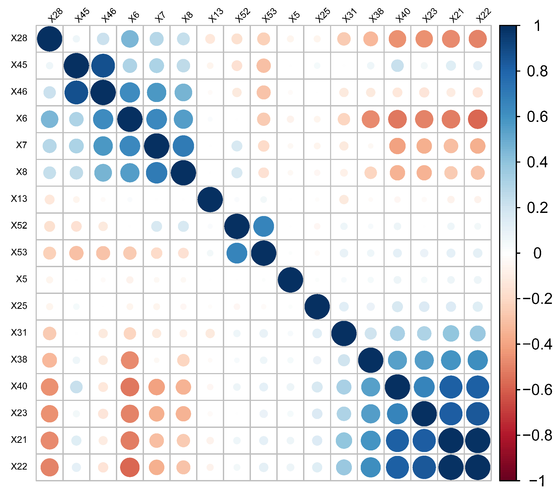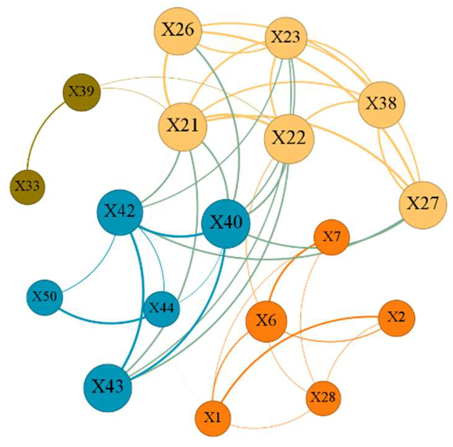In Section 4, we focus on empirical analysis by selecting financial indicators of listed companies. This section primarily covers the selection of financial indicators, the analysis of correlation among these indicators, the model’s results, and prediction analysis. Finally, in Section 5, we offer a summary of our findings and provide an outlook for future research.

2. Methods

2.1. Cox Proportional Hazards Model and Its Transformation

The Cox proportional hazards model can be formulated in terms of $({\tilde{T}}_i,{\delta }_i,X_i)$ for $i=1,\dots ,n$. Assuming a sample of n independent observations, ${\delta }_i=I\left({\tilde{T}}_i\le C_i\right)$, ${\tilde{T}}_i=\min$$\left(T_i,C_i\right)$, T and C represent the survival time and censoring time of individual i, respectively, and they are independent of each other. The event indicator variable is denoted by ${\delta }_i$, where ${\delta }_i=1$ indicates that the sample has experienced a financial risk, and ${\delta }_i=0$ indicates that the sample has not experienced a financial risk. The structural expression of the Cox proportional hazards model is as follows:

$$h_i\left(t;x\right)=h_0\left(t\right)\exp \left({\beta }^T{x}_i\right),$$

(1)

where $h_i\left(t;x\right)$ is the risk rate function of object i at time t. $h_0\left(t\right)$ is an unspecified benchmark risk function that represents the hazard rate of a company’s financial risk when all covariates are zero, and vector $x_i={(x_{i1},\dots x_{ip})}^T$ represents the p-lattice covariate indicators of company i. It is assumed that all covariate indicators have been standardized so that ${\displaystyle \sum _{i=1}^n{x}_{ij}}=0$, $\frac{1}{n}{\displaystyle \sum _{i=1}^n{x}_{ij}^2}=1$, $\beta =({\beta }_1,\dots {\beta }_p{)}^T$ is the set of p regression coefficients to be estimated. When ${\beta }_i>0$, $x_i$ represents the risk factor, and as the value of $x_i$ increases, the risk rate of financial risk for the company also increases. On the other hand, when ${\beta }_i<0$, $x_i$ represents the protection factor, and as the value of $x_i$ increases, the risk rate of financial risk for the company decreases. Assuming that among n samples, m companies have experienced financial risk, and the event occurrence times do not overlap, $t_1<t_2<\dots <t_m$. The regression coefficients are estimated using the partial likelihood function estimation method, and the log-partial likelihood function is as follows:

$$L\left(\beta \right)={\displaystyle \prod }_{i=1}^m\frac{e^{{\beta }^T{x}_i}}{{\displaystyle {\sum }_{j\in R_i}{e}^{{\beta }^T{x}_j}}}.$$

(2)

The set $R_i=\{j:{\tilde{T}}_j\ge {\tilde{T}}_i\}$ represents the collection of individuals who are still alive at the time of the i-th event, and its log-partial likelihood function is as follows:

$${\ell }_n\left(\beta \right)={\displaystyle \sum _{i=1}^n{\delta }_i}\left[{\beta }^T{x}_i-log\left({\displaystyle {\sum }_{j\in R_i}\exp ({\beta }^T{x}_j)}\right)\right].$$

(3)

The loss function is the negative of Equation (3). Due to the absence of a closed-form solution for the logarithmic partial likelihood function of the Cox model, this paper employs the coordinate descent method proposed by Friedman et al. [31] and converts the Cox model into a weighted least squares form for solution. Here, $X$ denotes the design matrix, and $\beta$ represents the regression coefficient vector, $\eta =X\beta$, $\tilde{\eta }=X\tilde{\beta }$. The second-order Taylor expansion of Equation (3) at $\tilde{\beta }$ is given as follows:

$$\begin{array}{ll}\ell (\beta )& \approx \ell (\tilde{\beta })+{(\beta -\tilde{\beta })}^T{\ell }^{\prime }(\tilde{\beta })+\frac{1}{2}{(\beta -\tilde{\beta })}^T{\ell }^{″}(\tilde{\beta })(\beta -\tilde{\beta })\\ & =\ell (\tilde{\beta })+{(X\beta -\tilde{\eta })}^T{\ell }^{\prime }(\tilde{\eta })+\frac{1}{2}{(X\beta -\tilde{\eta })}^T{\ell }^{″}(\tilde{\eta })(X\beta -\tilde{\eta }),\end{array}$$

(4)

where $l^{\prime }(\beta )$, $l^{″}(\beta )$, $l^{\prime }(\eta )$, and $l^{″}(\eta )$ represent the slope and the Hessian matrix of the log-likelihood functions of $\beta$ and $\eta$, respectively. By simplifying Equation (4), we obtain the following expression:

$$\ell (\beta )\approx \frac{1}{2}{(z(\tilde{\eta })-X\beta )}^T{\ell }^{″}(\tilde{\eta })(z(\tilde{\eta })-X\beta )+C(\tilde{\eta },\tilde{\beta }),$$

(5)

where $z(\tilde{\eta })=\tilde{\eta }-{\ell }^{″}{(\tilde{\eta })}^{-1}\ell (\tilde{\eta })$, and $C(\tilde{\eta },\tilde{\beta })$ is a known constant independent of $\beta$. To simplify the calculation process, the diagonal matrix of $l^{″}(\eta )$ can be used instead of the Hessian matrix, and the i-th value on the diagonal of the $l^{″}(\eta )$ matrix is denoted by $\gamma ({\tilde{\eta }}_i)$. Thus, the weighted least squares form of $\ell (\beta )$ is obtained as follows:

$$\ell (\beta )\approx \frac{1}{2}{\displaystyle \sum _{i=1}^n\gamma ({\tilde{\eta }}_i){(z({\tilde{\eta }}_i)-{\beta }^T{x}_i)}^2}.$$

(6)

2.2. l₀ Regularization

In financial risk forecast models, certain financial indicators may not significantly affect a company’s survival time. The prediction results obtained using Equation (3) may not be reasonably interpretable. Therefore, a penalty function can be added to select appropriate indicators. In theory, the $l_0$ penalty function $P(\beta )={\lambda }_1{\displaystyle \sum _{i=1}^{p}I({\beta }_j\ne 0)}$ has the Oracle property under large samples. Hence, the $l_0$ penalty is incorporated into the model to construct the following Equation:

$$\widehat{\beta }=\underset{\beta }{\arg \min }\left\{-\frac{1}{n}\ell (\beta )+P(\beta ;{\lambda }_1)\right\}.$$

(7)

2.3. Graph Regularization

Although Equation (7) can select variables, it does not consider the interrelationships among variables. Ignoring these relationships, especially when variables have strong correlations, can negatively impact the results. Graph structures can effectively describe the complex relationships among variables. A graph structure is a complex network system consisting of nodes, edges, and edge weights. This information can be represented by a weighted graph $G=(V,E,W)$, where $V=\left\{1,\dots ,p\right\}$ is the node set, $E=\left\{i\sim j\right\}$ is the set of edges representing connections between nodes, and $W=(w_{ij}),(i,j)\in E$ represents the weight of the edges. Additionally, let $d_i={\displaystyle {\sum }_{i(i,j)\in E}{w}_{ij}}$ denote the degree of each vertex, which represents its connectivity. We define the normalized Laplacian matrix L of the graph as follows:

$$l_{ij}=\{\begin{array}{c}\hspace{1em}1-w_{ii}/d_i \hspace{1em}\hspace{1em}\mathrm{if} i=j \mathrm{and} d_i\ne 0,\\ -w_{ij}/\sqrt{d_i{d}_j} \hspace{1em}\hspace{1em}\hspace{1em}(i,j\in E),\\ 0 \hspace{1em}\hspace{1em}\hspace{1em}\hspace{1em}\hspace{1em}\hspace{1em}\mathrm{otherwise}. \end{array}$$

(8)

This paper considers an undirected graph structure represented by a symmetric adjacency matrix $W={\left[w_{ij}\right]}_{p\times p}$, where the Pearson correlation coefficient $r_{ij}$ denotes the relationship between $X_i$ and $X_j$. $w_{ij}=\left|r_{ij}\right|I\left\{\left|r_{ij}\right|>r\right\}$. The determination of the threshold value involves utilizing the Fisher transformation and a statistical quantity of $f_{ij}=0.5\log ((1+r_{ij})/(1-r_{ij}))$. When the correlation between $X_i$ and $X_j$ is 0, the distribution of $\sqrt{n-3}{f}_{ij}$ approximates the standard normal distribution $N(0,1)$. The threshold value $c$ for $r_{ij}$ is determined via a hypothesis test, the threshold of $r_{ij}$ is $r=\frac{\exp (2c/\sqrt{n-3})-1}{\exp (2c/\sqrt{n-3})+1}$ with the critical value $c$ representing the $\alpha -\mathrm{th}$ quantile of a normal distribution. As the critical value $c$ increases, the threshold value $r$ increases, resulting in a sparser adjacency matrix. In this paper, we set $\alpha$ to be 0.995, which corresponds to $c=2.58$. We add a second penalty term $P^{*}(\beta ,{\lambda }_2)={\beta }^T\tilde{L}\beta$ to Equation (7) and construct the GR-Cox model with a graph structure as follows:

$$\begin{array}{ll}\widehat{\beta }& =\underset{\beta }{\arg \min }\left\{-\frac{1}{n}\ell (\beta )+P(\beta ;{\lambda }_1)+P^{*}(\beta ,{\lambda }_2)\right\}\\ & =\underset{\beta }{\arg \min }\left\{-\frac{1}{n}\ell (\beta )+{\lambda }_1{\displaystyle \sum _{i=1}^{p}I({\beta }_j\ne 0)}+\frac{{\lambda }_2}{2}{\displaystyle \sum _{(i,j)\in E}{w}_{ij}{\left(\frac{\mathrm{sgn}({\tilde{\beta }}_i){\beta }_i}{\sqrt{d_i}}-\frac{\mathrm{sgn}({\tilde{\beta }}_j){\beta }_j}{\sqrt{d_j}}\right)}^2}\right\},\end{array}$$

(9)

where $\tilde{L}=({\tilde{l}}_{ij})=S^{T}LS$,$S=\mathrm{diag}(\mathrm{sgn}({\tilde{\beta }}_1),\dots ,\mathrm{sgn}({\tilde{\beta }}_p))$. The sign of coefficient $\tilde{\beta }=({\tilde{\beta }}_1,\dots ,{\tilde{\beta }}_p)$ is obtained from prior information. Equation (9) consists of two penalty terms with distinct functions. The first term is the $l_0$ penalty that promotes model sparsity for variable selection, while the second term is a graph structure penalty that employs graph structure to smooth out the coefficient differences between related variables and mitigate the negative impact of multicollinearity. $\mathrm{sgn}({\tilde{\beta }}_i){\beta }_i$ is utilized to approximate $\left|\beta \right|$. If the explanatory variables $X_i$ and $X_j$ exhibit high connectivity in the graph structure (i.e., large $w_{ij}$), the corresponding penalty weight will be significant, leading to more similar magnitudes of their coefficient absolute values. To reduce excessive penalties on crucial variables and the resultant additional bias, we scale the coefficients by the square root of the vertex degree.

The initial value of $\tilde{\beta }$ can be obtained from the ridge regression estimation results. Compared to methods like LASSO and Elastic Net, ridge regression compresses the model parameter values to a lesser extent but does not shrink any coefficient to 0. Thus, it avoids the loss of node and edge information [32]. Hence, we obtain the initial value of $\tilde{\beta }$ using the following Equation (10):

$$\tilde{\beta }=\underset{\beta }{\arg \min }\left\{-\frac{1}{n}\ell (\beta )+\lambda {\displaystyle \sum _{j=1}^p{\beta }_j{}^2}\right\}.$$

(10)

2.4. Calculation Methods

Due to the discontinuity of the $l_0$ penalty term in Equation (9), it becomes an NP-hard problem to directly estimate this term in high-dimensional cases, leading to a significant increase in computation [33]. To address this issue, this paper adopts a method proposed by Li et al. [34] and introduces a surrogate parameter $\theta$ that approximates $\beta$ and $\theta$ in a convex function, thereby transforming the problem of solving $\beta$ into the problem of solving $\theta$. Additionally, a convex function $\varphi (x)=x^2$ is constructed to facilitate the optimization process, which satisfies $\varphi (0)=0$ and $\varphi (\left|x\right|)\ge 0(x\ne 0)$. Thus, the penalty problem is transformed as follows:

$$(\widehat{\beta },\widehat{\theta })=\arg \min \left\{-\frac{1}{n}\ell (\beta )+{\lambda }_1{\displaystyle \sum _{j=1}^{p}I({\theta }_j\ne 0)}+\frac{{\lambda }_2}{2}{\displaystyle \sum _{(i,j)\in E}{w}_{ij}{\left(\frac{\mathrm{sgn}({\tilde{\beta }}_i){\beta }_i}{\sqrt{d_i}}-\frac{\mathrm{sgn}({\tilde{\beta }}_j){\beta }_j}{\sqrt{d_j}}\right)}^2}\right\},$$

$$\mathrm{s}. \mathrm{t}. {\displaystyle \sum _{j=1}^p\varphi }(\left|{\beta }_j-{\theta }_j\right|)\le m,$$

(11)

where $m$ is an adjustment parameter, and the smaller $m$ is, the closer $\beta$ and $\theta$ are under the $\varphi (\cdot )$ function. Equation (11) is equivalent to finding the minimum value of the following problem:

$$L_{{\lambda }_1,{\lambda }_2,{\lambda }_3}\left(\beta ,\theta \right)=-\frac{1}{n}l\left(\beta \right)+{\lambda }_1{\displaystyle \sum }_{j=1}^{p}I\left({\theta }_j\ne 0\right)+\frac{{\lambda }_2}{2}{\displaystyle \sum _{(i,j)\in E}{w}_{ij}{\left(\frac{\mathrm{sgn}({\tilde{\beta }}_i){\beta }_i}{\sqrt{d_i}}-\frac{\mathrm{sgn}({\tilde{\beta }}_j){\beta }_j}{\sqrt{d_j}}\right)}^2}+{\lambda }_3{\displaystyle \sum }_{j=1}^p\varphi \left(\left|{\beta }_j-{\theta }_j\right|\right),$$

(12)

where ${\lambda }_1$, ${\lambda }_2$, and ${\lambda }_3$ are non-negative Lagrange adjustment parameters. For the selection of each parameter, cross-validation is used to choose the optimal $\lambda$ according to the principle of minimizing the test set average cross-validation partial likelihood. The minimization process of Equation (12) is divided into two parts, each corresponding to an optimization problem: solving $\beta$ and $\theta$.

$$\widehat{\beta }=\underset{\beta }{\mathrm{argmin}}\left\{-\frac{1}{n}l\left({\beta }_0,\beta \right)+\frac{{\lambda }_2}{2}{\displaystyle \sum _{(i,j)\in E}{w}_{ij}{\left(\frac{\mathrm{sgn}({\tilde{\beta }}_i){\beta }_i}{\sqrt{d_i}}-\frac{\mathrm{sgn}({\tilde{\beta }}_j){\beta }_j}{\sqrt{d_j}}\right)}^2}+{\lambda }_3{\displaystyle \sum }_{j=1}^p\varphi \left(\left|{\beta }_j-{\theta }_j\right|\right)\right\},$$

(13)

$$\widehat{\theta }=\arg \underset{\theta }{\min }\left\{{\lambda }_1{\displaystyle \sum }_{j=1}^{p}I\left({\theta }_j\ne 0\right)+{\lambda }_3{\displaystyle \sum }_{j=1}^p\varphi \left(\left|{\beta }_j-{\theta }_j\right|\right)\right\}.$$

(14)

This paper uses coordinate descent to solve Equation (13). The core strategy of this algorithm is to update only one coefficient at a time (denoted as ${\beta }_k$) while keeping the other coefficients fixed. Then, estimate ${\theta }_k$ through hard thresholding ${\widehat{\theta }}_k={\widehat{\beta }}_{j}I\left(\varphi \left(\left|{\widehat{\beta }}_k\right|\right)>{\lambda }_1/{\lambda }_3\right),j=1,\dots ,p$. For the updated ${\beta }_k$, the iterative formula is obtained by taking the derivative and organizing the three terms in Equation (13) as follows:

$${\widehat{\beta }}_k=\frac{-\frac{1}{n}{{\displaystyle \sum }}_{i=1}^n{\gamma }_i{x}_{ij}{H}_{i,-k}+2{\lambda }_3{\widehat{\theta }}_k+{\lambda }_2{\displaystyle \sum _{i=1}^{k-1}{w}_{ik}\frac{\mathrm{sgn}({\tilde{\beta }}_i)}{\sqrt{d_i}}}\frac{\mathrm{sgn}({\tilde{\beta }}_k)}{\sqrt{d_k}}{\beta }_i+{\lambda }_2{\displaystyle \sum _{j=k+1}^p{w}_{kj}}\frac{\mathrm{sgn}({\tilde{\beta }}_j)}{\sqrt{d_j}}\frac{\mathrm{sgn}({\tilde{\beta }}_k)}{\sqrt{d_k}}{\beta }_j}{-\frac{1}{n}{\displaystyle \sum _{i=1}^n{\gamma }_i{x}_{ik}^2}+2{\lambda }_3+{\lambda }_2{\displaystyle \sum _{i=1}^{k-1}{w}_{ik}\frac{1}{d_k}+{\lambda }_2{\displaystyle \sum _{j=k+1}^p{w}_{kj}}\frac{1}{d_k}}},$$

(15)

where $H_{i,-k}=z({\tilde{\eta }}_i)-{\beta }_{-k}^T{x}_{i,-k}$. The algorithm is shown in

Table 1. Algorithm.

Flow of the Algorithm
Initialize $\widehat{\beta }=\widehat{\eta }=0$ and set the iteration number $s=0$. (1)Fix $\widehat{\beta }={\widehat{\beta }}^{(s)}$, update ${\widehat{\theta }}^{(s+1)}$ with iterative update Equation (14). (2)Fix $\theta ={\widehat{\theta }}^{(s+1)}$, update ${\widehat{\beta }}^{(s+1)}$ with iterative Equation (15). $s=s+1$. Loop step 2 and step 3 until convergence, the convergence criterion is that the maximum value of the difference between two adjacent parameter estimates does not exceed ${10}^{-5}$.

.

3. Numerical Simulation

3.1. Generation of Data

In order to verify the effectiveness of the GR-Cox method proposed in this paper for the indicator selection, we conducted Monte Carlo numerical simulations. The independent variable was $X\sim N\left(0,\sum \right)$, $\sum ={(r_{ij})}_{p\times p}$. Financial status was randomly generated from a Bernoulli distribution with a probability of 0.7, and the survival time was randomly generated from an exponential distribution $E({\mathrm{e}}^{{\beta }^T{x}_i})$. Two commonly used types of correlation were considered. The first type was the autoregressive (AR) correlation structure, with $r_{ij}=r^{\left|i-j\right|}$, and three correlation coefficients of 0.2, 0.5, and 0.7 representing weak, moderate, and strong correlations, respectively. The second type was the banded correlation (BC) structure, with $r_{ij}=0.33$ when $\left|j-i\right|=1$ for BC (1), $r_{ij}=0.6$ when $\left|j-i\right|=1$, and $r_{ij}=0.33$ when $\left|j-i\right|=2$ for BC (2), and $r_{ij}=0$ otherwise. In the simulation, the absolute values of the coefficients between adjacent variables were similar, with $p=80$, $n=300$, and $\beta =(X_1,X_2,X_3,X_4,$$X_5,X_6,X_7,X_8,\underset{72}{\underbrace{0,\mathrm{...0}}}{)}^T$. The coefficients of significant variables were randomly generated from a uniform distribution $U(0.5,1.2)$, and their signs were randomly produced from a 0–1 distribution with a probability of 0.5.

3.2. Indicator Assessment

In order to verify the variable selection performance of the proposed GR-Cox model, three other comparative models were selected in this paper, including the LASSO-Cox model with $l_1$ penalty, the Cox-$l_0$ model without network structure, and the Cox-ENet model with elastic net penalty. The following evaluation metrics were used to evaluate the overall performance of the models: the number of true positives (TP) which are correctly selected non-zero coefficients, the number of false positives (FP) which are incorrectly selected non-zero coefficients, and the model error rate ($error=(FP+FN)/n$). FP represents the number of false positives, while FN represents the number of false negatives. The mean results of 100 repeated simulations are shown in

Table 2. Results of the simulation.

Correlation	Model	TP	FP	Error
AR (0.2)	GR-Cox	7.91 (0.32)	0.49 (1.80)	0.01 (0.02)
	COX-LASSO	8.00 (0.00)	13.91 (2.91)	0.17 (0.03)
	COX-$l_0$	7.70 (0.20)	0.24 (0.66)	0.01 (0.01)
	COX-ENet	8.00 (0.00)	13.49 (3.29)	0.16 (0.04)
AR (0.5)	GR-Cox	7.92 (0.25)	0.84 (3.00)	0.01 (0.03)
	COX-LASSO	7.93 (0.30)	12.18 (12.18)	2.99 (0.15)
	COX-$l_0$	6.67 (0.56)	0.55 (0.74)	0.02 (0.01)
	COX-ENet	7.91 (0.28)	12.58 (3.01)	0.15 (0.03)
AR (0.7)	GR-Cox	7.54 (0.74)	0.73 (1.39)	0.01 (0.01)
	COX-LASSO	7.28 (0.51)	9.61 (2.89)	0.12 (0.03)
	COX-$l_0$	4.06 (0.81)	0.66 (0.92)	0.05 (0.01)
	COX-ENet	7.74 (0.59)	11.78 (3.08)	0.15 (0.04)
BC (1)	GR-Cox	7.60 (0.66)	0.47 (2.00)	0.01 (0.01)
	COX-LASSO	7.95 (0.21)	10.88 (2.13)	0.06 (0.02)
	COX-$l_0$	7.59 (0.43)	0.85 (0.79)	0.02 (0.02)
	COX-ENet	7.97 (0.17)	13.58 (3.06)	0.17 (0.03)
BC (2)	GR-Cox	7.79 (0.73)	0.08 (0.36)	0.01 (0.01)
	COX-LASSO	7.90 (0.33)	11.69 (2.92)	0.14 (0.03)
	COX-$l_0$	5.67 (0.82)	1.22 (1.33)	0.04 (0.01)
	COX-ENet	7.73 (0.48)	10.68 (2.73)	0.13 (0.03)

with the standard deviation in parentheses.

3.3. Analysis of the Simulation Results

According to Table 2, the variable selection error of GR-Cox is superior to that of the comparison models, with the lowest error value among all models, indicating that the model has good stability. The GR-Cox model with a graph structure selects more true positives (TP) than the model without a graph structure. As the correlation between variables increases, the number of correctly selected variables by the GR-Cox model is higher than that of Cox-LASSO and Cox-ENet. For example, when the correlation coefficient is AR (0.7), the TP value of GR-Cox (7.54) is higher than that of Cox-LASSO (7.28) and Cox-$l_0$ (4.06). The FP value of GR-Cox (0.73) is slightly higher than that of the Cox-$l_0$ model (0.66), but much lower than that of Cox-LASSO (9.61) and Cox-ENet (11.78). Meanwhile, the error value of the GR-Cox model (0.01) is significantly lower than that of Cox-LASSO (0.12), Cox-$l_0$ (0.05), and Cox-ENet (0.15). This indicates that adding the correlation between variables to the model can improve the selection accuracy. Although the TP values of Cox-LASSO and Cox-ENet are slightly higher than that of GR-Cox in specific cases, this is achieved at the expense of higher FP values. As shown in Table 2, when the correlation coefficient is AR (0.2), although Cox-LASSO and Cox-ENet models select eight significant coefficient variables, their FP values are significantly higher than the GR-Cox model (0.49). In both AR-type and BC-type correlations, the GR-Cox model performs well. Overall, the GR-Cox model accurately selects variables while reducing the number of false positives.

4. Empirical Analysis of Financial Risk Early Warning

4.1. Selection of Financial Indicators

The data used in this study were obtained from the China Stock Market and Accounting Research (CSMAR) database. During the sample selection process, we performed the following data processing: (1) we excluded companies in the financial and insurance industries, which usually have significant differences from companies in other industries, including the calculation methods of financial indicators, the structure of assets, and the nature of revenues and expenses. Therefore, excluding the financial and insurance industries can reduce interference when constructing the model, making the analysis more accurate and reliable. (2) We excluded companies that were delisted before being ST or before the end of the observation period. (3) We removed the companies with missing data. The observation period ended on 31 December 2022. During this period, a total of 826 companies were selected from the A-share market, including 272 ST companies and 554 non-ST companies. Random sampling was used to select 70% of the data as the training set to train the model, while the remaining 30% was used as the test set to assess the model’s predictive performance. For companies that have been ST, their survival time was measured from their listing date to the first occurrence of being ST. For non-ST companies, their survival time was measured from their listing date to December 31, 2022. Based on the relevant ST policy provisions, listed companies that become ST will exhibit a downward trend in financial indicators during the first two years. To test the model’s predictive ability, this study uses financial data of listed companies T-2 for financial risk early warning. Drawing on a comprehensive analysis of existing literature and referencing Zhang et al. [35], this study selects 54 financial indicators covering seven aspects, as shown in

Table 3. Selection of indicators.

Classification of Indicators	Indicators
Solvency	$X_1$ Current ratio; $X_2$ Conservative quick ratio; $X_3$ Cash ratio; $X_4$ Working capital; $X_5$ Interest coverage multiple; $X_6$ Gearing ratio; $X_7$ Equity ratio; $X_8$ Long-term debt-to-equity ratio; $X_9$ Long-term debt-to-working capital ratio; $X_{10}$ Net cash flow from operating; $X_{11}$ Debt to tangible assets ratio
Operating Capacity	$X_{12}$ Inventory to revenue ratio; $X_{13}$ Operating cycle; $X_{14}$ Accounts payable turnover ratio; $X_{15}$ Cash and cash equivalents turnover ratio; $X_{16}$ Current assets turnover ratio; $X_{17}$ Fixed assets turnover ratio; $X_{18}$ Non-current assets turnover ratio; $X_{19}$ Capital intensity; $X_{20}$ Total assets turnover ratio
Profitability	$X_{21}$ Return on total assets; $X_{22}$ Return on assets; $X_{23}$ Net profit margin on current assets; $X_{24}$ Net profit margin on fixed assets; $X_{25}$ Earnings before interest and tax; $X_{26}$ Return on invested capital; $X_{27}$ Long-term return on capital; $X_{28}$ Operating cost ratio
Cash Flow	$X_{29}$ Cash content of operating income; $X_{30}$ Corporate cash flow; $X_{31}$ Total cash recovery rate
Development Capacity	$X_{32}$ Growth rate of fixed assets; $X_{33}$ Growth rate of total assets; $X_{34}$ Growth rate of operating income; $X_{35}$ Growth rate of total operating costs; $X_{36}$ Growth rate of selling expenses; $X_{37}$ Growth rate of administrative expenses; $X_{38}$ Sustainable growth rate; $X_{39}$ Growth rate of owner’s equity
Per Share Metrics	$X_{40}$ Earnings per share; $X_{41}$ Total operating income per share; $X_{42}$ Earnings before interest and taxes per share; $X_{43}$ Operating income per share; $X_{44}$ Net asset value per share; $X_{45}$ Tangible assets per share; $X_{46}$ Debt per share; $X_{47}$ Net cash flow from investing activities per share; $X_{48}$ Depreciation and amortization per share; $X_{49}$ Net cash flow per share; $X_{50}$ Net assets per share attributable to the parent company
Relative Value Metrics	$X_{51}$ Price-to-sales ratio; $X_{52}$ Price-to-book Ratio; $X_{53}$ Tobin’s Q; $X_{54}$ Book-to-market ratio

.

4.2. Descriptive Statistical Analysis

To explore the correlation among variables, we first conducted a correlation analysis. as shown in

Table 4. Correlation coefficient distribution.

Scope	Value
Below 0.2	81.97%
0.2–0.5	12.43%
Above 0.5	5.59%

. The results indicate that 81.97% of the correlation coefficients between explanatory variables are below 0.2, while 12.43% are between 0.2 and 0.5, and 5.59% are above 0.5.

As shown in Figure 1, there are significant correlations between return on total assets ($X_{21}$) and return on assets ($X_{22}$) (0.80), return on total assets ($X_{21}$) and net profit margin on current assets ($X_{23}$) (0.76), return on assets ($X_{22}$) and net profit margin on current assets ($X_{23}$) (0.82), as well as between equity ratio ($X_7$) and long-term debt-to-equity ratio ($X_8$) (0.98). Therefore, it is necessary to consider the correlation among variables in the process of variable selection.

In order to analyze the relationships among variables, this study constructed a variable relationship graph based on complex network theory and an adjacency matrix. Different colors represent different modules, and the size of each node represents the degree size $d_i$. The larger the node, the greater the weighted average degree between the node and its neighboring nodes, indicating that the node is more important in the graph. As shown in Figure 2, the more important nodes in the graph structure are $X_{22}$, $X_{40}$, $X_{21}$, $X_{27}$, $X_{42}$, etc.

Module partitioning divides a complex network into multiple modules so that the connections within modules are tight and the connections between modules are sparse. The nodes in the same module tend to have similar properties. As seen in Figure 2, the more important financial indicators are divided into four modules. The following financial indicators are classified into the same module and represented in yellow: return on total assets, return on assets, net profit margin on current assets, return on invested capital, long-term return on capital, and sustainable growth rate. Earnings per share, earnings before interest and taxes per share, operating income per share, net asset value per share, and net assets per share attributable to the parent company are divided into another module, indicated in blue.

4.3. Estimation of Coefficients for Financial Risk Warning Model

After variable selection using the GR-Cox model, 10 out of 54 indicators were selected for further analysis. The selected variables were subjected to likelihood ratio, Wald, and score tests. The likelihood ratio test was used to examine whether adding a new independent variable to the model would significantly improve its explanatory power. The Wald and score tests were used to examine whether a specific variable had a significant impact on survival analysis. The results of the tests are presented in

Table 5. Tests of the model.

Tests	Chi-Square Value	Degrees of Freedom	p-Value
Likelihood ratio	169.8	10	<2.2$\times e^{-16}$
Wald	144.3	10	<2.2$\times e^{-16}$
Score	173.3	10	<2.2$\times e^{-16}$

.

Based on Table 5, all three tests are statistically significant at $\alpha =0.05$.

Table 6. Coefficients of the model.

Variable	GR-Cox	Cox-LASSO	$\mathbf{Cox}-{\mathit{l}}_0$	Cox-ENet
$X_6$	0.173	0.164	0.468	0.096
$X_7$	0.054	0.048	-	0.071
$X_{11}$	-	-	−0.982	-
$X_{21}$	−0.164	−0.145	−0.237	−0.094
$X_{22}$	−0.242	−0.224	−0.304	−0.122
$X_{23}$	−0.248	−0.237	-	−0.153
$X_{25}$	-	-	-	−0.002
$X_{26}$	−0.031	−0.040	-	−0.071
$X_{27}$	-	-	-	−0.042
$X_{28}$	0.013	0.001	-	0.010
$X_{31}$	−0.062	−0.031	−0.271	-
$X_{33}$	-	-	0.252	-
$X_{38}$	−0.008	−0.035	-	−0.100
$X_{40}$	−0.072	−0.060	-	−0.053
$X_{47}$	-	-	−0.221	-
$X_{52}$	-	-	0.265	-
$X_{54}$	-	-	0.213	-

shows the coefficients obtained via the model, from which it can be seen that the GR-Cox comparative model selected 10, 9, and 11 variables, respectively. The four models have consistent coefficient signs and similar estimated values, with three overlapping variables: gearing ratio, return on total assets, and return on assets. Regarding the practical significance of the selected indicators, the coefficient of the $X_6$ gearing ratio is 0.173, indicating that for every unit increase in the company’s gearing ratio, the degree of financial risk increases by a factor of $e^{0.173}$ (1.189) times. In economic terms, the gearing ratio is calculated as the total liabilities divided by total assets. A higher value indicates lower solvency and higher operational risk. Additionally, the coefficient of $X_7$ (equity ratio) is positive (0.054), indicating that for every unit increase in the equity ratio, the degree of financial risk increases by a factor of $e^{0.054}$ (1.055) times. Similarly, the degree of financial risk increases by $e^{\beta i}$ times for every unit increase in the growth rate of the operating cost ratio. However, $X_{21}$ (return on total assets), $X_{22}$ (return on assets), and $X_{26}$ (return on invested capital) have negative coefficients (−0.164, −0.242, and −0.031), indicating that they protect the company’s financial condition. Every unit increase in these indicators reduces the degree of financial risk by a factor of $1-e^{{\beta }_i}$ times. Similar conclusions were drawn in the research by Huang et al. [17] and Jairaj Gupta et al. [36]. Overall, the selected indicators in the model align with their real economic significance.

4.4. Survival Probability Estimation

The survival status of a company can be reflected through the estimated survival probability. Therefore, the survival function is established as follows:

$$S(t|X)=S_0{(t)}^{{\exp }^{{\beta }^T{x}_i}}.$$

(16)

where $S_0(t)=\exp \left(-{\displaystyle {\int }_0^t{h}_0(u) du}\right)$ is the benchmark survival function, $H_0(t)={\displaystyle {\int }_0^t{h}_0\left(\mathrm{u}\right) }du$. This paper uses the Breslow method ${\widehat{H}}_0(t)={\displaystyle \sum _{t(i)<t}\frac{1}{{\displaystyle \sum _{j\in R_i}\exp ({\beta }^T{x}_i)}}}$ to estimate $H_0(t)$. The benchmark survival function ${\widehat{S}}_0(t)$ is further obtained, as shown in

Table 7. Baseline survival functions.

$t$	3	4	5	6	7	8
${\widehat{S}}_0\left(t\right)$	0.996	0.989	0.984	0.975	0.958	0.940
$t$	9	10	11	12	13	14
${\widehat{S}}_0\left(t\right)$	0.925	0.903	0.885	0.869	0.843	0.812
$t$	15	16	17	18	19	20
${\widehat{S}}_0\left(t\right)$	0.782	0.749	0.713	0.690	0.665	0.635
$t$	21	22	23	24	25+
${\widehat{S}}_0\left(t\right)$	0.621	0.553	0.535	0.512	0.459

. Finally, the estimate of the survival probability of the listed company can be obtained according to $\widehat{S}(t|X=X^{\ast })={\widehat{S}}_0{(t)}^{{\exp }^{{\beta }^T{x}_i}}$.

4.5. Classification Prediction Evaluation

The GR-Cox model is employed to estimate the survival probability, which is then compared to the critical value $C_t$ that represents the financial risk occurrence. If the predicted survival probability of a company is $\widehat{S}(t|X)<C_t$, then the company is considered to be in a financial risk; otherwise, it is deemed not to be experiencing a financial risk. Lane [13] suggested that $C_t$ should be equal to the proportion of non-distressed companies in the sample, calculated as the number of companies with normal financial conditions at time t divided by the total number of sample companies. The GR-Cox model, along with three other comparison models, was trained on a training set and tested on a testing set. The results are presented in

Table 8. Model prediction results.

Models	Categories	Classification Accuracy
		Training Set(%)	Test Set(%)
GR-Cox	ST Sample	84.36	82.80
	Non-ST sample	88.47	87.10
	All sample	87.20	85.48
Cox-LASSO	ST Sample	82.12	81.72
	Non-ST sample	88.22	85.81
	All sample	86.33	84.27
Cox-$l_0$	ST Sample	83.80	77.42
	Non-ST sample	79.95	78.71
	All sample	81.14	78.23
Cox-ENet	ST Sample	79.89	78.49
	Non-ST sample	85.71	84.52
	All sample	83.91	82.26

. Among the four models, the GR-Cox model achieved the highest overall accuracy for all samples, with accuracy rates of 87.20% on the training set and 85.48% on the testing set. To minimize the loss caused by misjudgment, accurately predicting non-ST samples is crucial. For the non-ST samples in the training set, the accuracy of Cox-LASSO, Cox-$l_0$, and Cox-ENet was 88.22%, 79.95%, and 85.71%, respectively, all of which were lower than that of the GR-Cox model. Similarly, in the testing set, the accuracy of Cox-LASSO, Cox-$l_0$, and Cox-ENet for non-ST samples was 85.81%, 78.71%, and 84.52%, respectively, also lower than that of the GR-Cox model. On the other hand, for ST samples, the accuracy of the GR-Cox model was higher compared to that of the comparison models, with an accuracy of 84.36% and 82.80%, respectively. Therefore, the proposed GR-Cox model demonstrates good predictive accuracy, and its performance is superior to that of the three comparison models.

The Cox model can discern the financial condition of listed companies and make time-point predictions. In this study, two companies with the stock codes 600319 and 002086 were randomly selected from the test set to represent the ST category during the observation period. Additionally, two other companies, namely 600018 and 002050, were chosen to represent the non-ST category during the same observation period. The GR-Cox model was utilized to calculate their predicted survival probability for more than t years during the observation period. The results of this analysis are depicted in Figure 3. It is evident that 600319 maintained a stable financial situation in the first 9 years of the observation period, with its survival probability consistently at a high level. However, in the first two years of the financial risk, its predicted survival probability significantly declined, dropping to less than 30% in the 12th year. Similarly, the survival probability of 002086 also experienced a substantial decline starting from the 11th year. The probability of surviving longer than 14 years in the observation period was merely 10.92%. This outcome aligns with the actual occurrence of the company’s financial risk in the 14th year. Conversely, the survival probabilities of companies with stock codes 600018 and 002050, which have not encountered financial crises, have consistently remained at a relatively high level. Therefore, it can be concluded that the GR-Cox model demonstrates the capability to accurately predict a company’s survival probability.

5. Conclusions

The presence of correlation information between financial indicators may affect the accuracy of classic financial early warning models in the area of financial risk early warning systems. To address this issue, a complex network theory is utilized to construct a graph structure based on the sample information of financial indicators. This approach not only captures the level of correlation between two financial indicators but also the interconnections within the system where all indicators are situated. This paper presents the GR-Cox model, which integrates the graph network structure into the Cox proportional hazards model. Variable selection is accomplished via $l_0$ regularization, and a quadratic approximation is employed for the partial likelihood function of Cox. An alternative parameter is introduced for the solution, and a coefficient estimation is performed using the coordinate descent algorithm. Simulation results demonstrate the superior indicator selection effect and accuracy of the GR-Cox model compared to the comparison models.

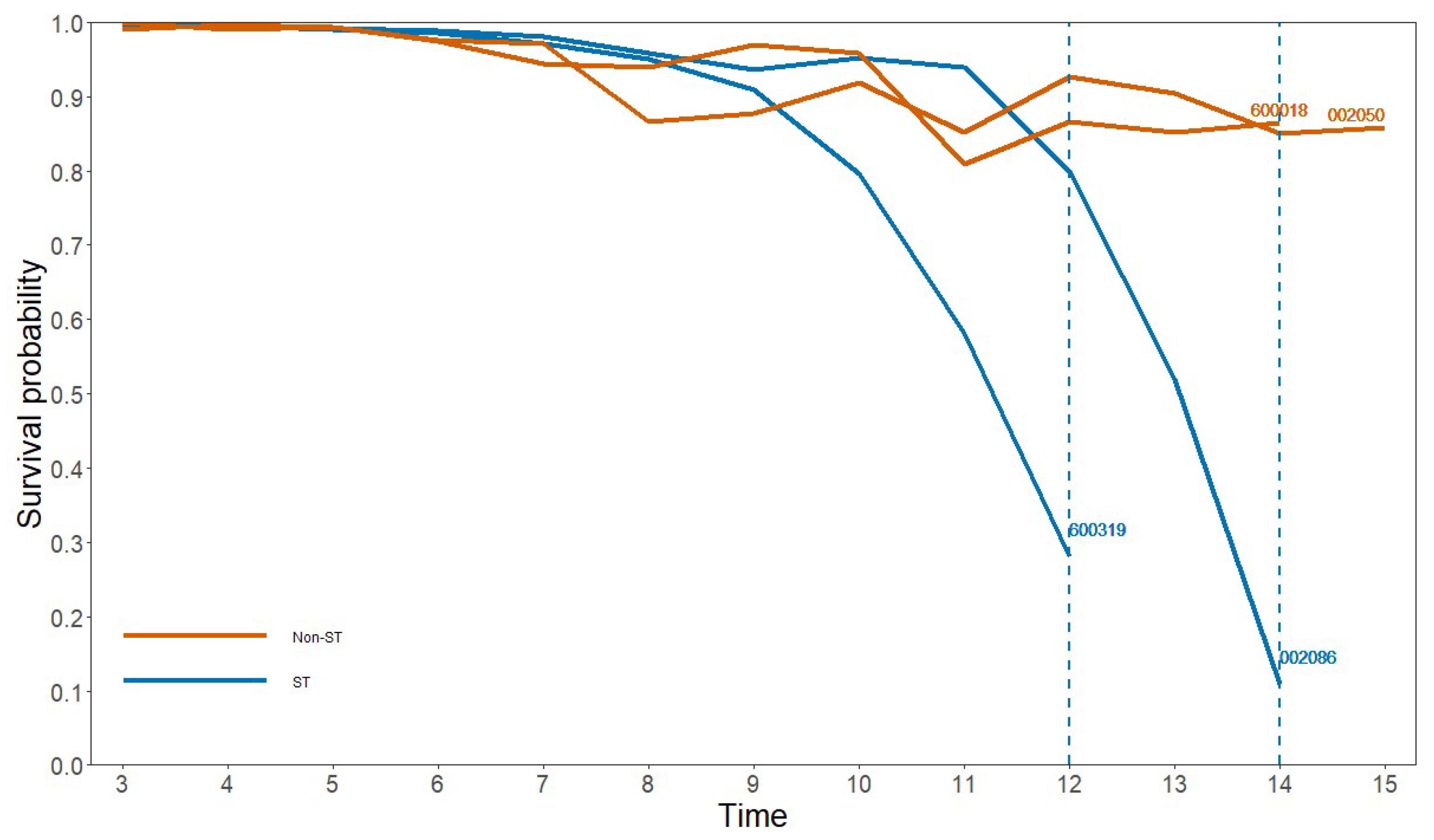
We analyzed 826 companies using 54 indicators from seven aspects. Ultimately, 10 indicators were included in the final financial risk prediction model. The model passed the likelihood ratio, Wald, and score tests. Specifically, the GR-Cox model selected two indicators from the solvency category, five indicators from the profitability category, and one indicator each from the cash flow, development capacity, and per share metrics categories. The coefficients of the gearing ratio, equity ratio, and operating cost ratio were 0.173, 0.054, and 0.013, respectively, indicating their positive impact on the likelihood of financial risk in listed companies. Increasing the values of these financial indicators would lead to a higher probability of financial risk. On the other hand, increasing the values of the remaining seven financial indicators will reduce the probability of a company’s financial risk. It is important for company managers, investors, and creditors to closely monitor these financial indicators and make appropriate adjustments when assessing the potential for future financial distress. Empirical research demonstrates that the GR-Cox model possesses the capability to dynamically forecast the survival probability of companies. During the initial years of a company’s listing, its survival probability remains at a relatively high level. However, as the operational pressures on the company intensify, if it encounters a financial risk, the GR-Cox model can accurately calculate the decrease in the survival probability. Compared with other models, our model exhibits high accuracy for both ST and non-ST samples, showcasing its outstanding predictive performance.

This study offers several avenues for further exploration. The prior coefficients of the model are obtained from ridge regression estimation, but more effective prior information can be obtained via other methods in future studies. Additionally, other penalties such as SCAD and MCP can be applied in variable selection, or other group class penalties such as Group LASSO can be used. The proposed model can also be extended to other risk control areas. For example, in banking, insurance, and bond markets, the model can be used to assess customers’ credit risks, predict default probabilities, and assist institutions in making informed decisions. Furthermore, the model can be expanded to other areas such as supply chain finance, personal credit assessment, and bank bankruptcy prediction, providing accurate default warnings and risk management tools for various stakeholders.

References

1. Altman, E.I. Financial Ratios, Discriminant Analysis and the Prediction of Corporate Bankruptcy. J. Financ. 1968, 23, 589–609. [Google Scholar] [CrossRef]
2. Ohlson, J.A. Financial Ratios and the Probabilistic Prediction of Bankruptcy. J. Account. Res. 1980, 18, 109–131. [Google Scholar] [CrossRef] [Green Version]
3. Jabarin, M.; Nour, A.; Atout, S. Impact of macroeconomic factors and political events on the market index returns at Palestine and Amman Stock Markets (2011–2017). Invest. Manag. Financ. Innov. 2019, 16. [Google Scholar] [CrossRef] [Green Version]
4. Asa’d, I.A.A.; Nour, A.; Atout, S. The Impact of Financial Performance on Firm’s Value During COVID-19 Pandemic for Companies Listed in the Palestine Exchange (2019–2020). In Proceedings of the From the Internet of Things to the Internet of Ideas: The Role of Artificial Intelligence: Proceedings of EAMMIS 2022, Coventry, UK, 13–14 May 2022; pp. 529–551. [Google Scholar] [CrossRef]
5. Zhao, Y.; Lin, D. Prediction of Micro-and Small-Sized Enterprise Default Risk Based on a Logistic Model: Evidence from a Bank of China. Sustainability 2023, 15, 4097. [Google Scholar] [CrossRef]
6. Li, Z.Y.; Crook, J.; Andreeva, G. Chinese companies distress prediction: An application of data envelopment analysis. J. Oper. Res. Soc. 2014, 65, 466–479. [Google Scholar] [CrossRef] [Green Version]
7. García, V.; Marqués, A.I.; Sánchez, J.S.; Ochoa-Domínguez, H.J. Dissimilarity-Based Linear Models for Corporate Bankruptcy Prediction. Comput. Econ. 2017, 53, 1019–1031. [Google Scholar] [CrossRef]
8. Zhou, Q.P.; Wang, L.; Juan, L.; Zhou, S.G.; Li, L.L. The Study on Credit Risk Warning of Regional Listed Companies in China Based on Logistic Model. Discret. Dyn. Nat. Soc. 2021, 2021, 6672146. [Google Scholar] [CrossRef]
9. Wang, G.; Ma, J.; Yang, S. An improved boosting based on feature selection for corporate bankruptcy prediction. Expert Syst. Appl. 2014, 41, 2353–2361. [Google Scholar] [CrossRef]
10. Zhao, D.; Huang, C.; Wei, Y.; Yu, F.; Wang, M.; Chen, H. An Effective Computational Model for Bankruptcy Prediction Using Kernel Extreme Learning Machine Approach. Comput. Econ. 2017, 49, 325–341. [Google Scholar] [CrossRef]
11. Tavana, M.; Abtahi, A.R.; Di Caprio, D.; Poortarigh, M. An Artificial Neural Network and Bayesian Network model for liquidity risk assessment in banking. Neurocomputing 2018, 275, 2525–2554. [Google Scholar] [CrossRef]
12. Zeng, S.; Li, Y.; Yang, W.; Li, Y. A Financial Distress Prediction Model Based on Sparse Algorithm and Support Vector Machine. Math. Probl. Eng. 2020, 2020, 5625271. [Google Scholar] [CrossRef]
13. Lane, W.R.; Looney, S.W.; Wansley, J.W. An application of the cox proportional hazards model to bank failure. J. Bank. Financ. 1986, 10, 511–531. [Google Scholar] [CrossRef]
14. Im, J.K.; Apley, D.W.; Qi, C.; Shan, X. A time-dependent proportional hazards survival model for credit risk analysis. J. Oper. Res. Soc. 2012, 63, 306–321. [Google Scholar] [CrossRef]
15. Ding, A.A.; Tian, S.; Yu, Y.; Guo, H. A Class of Discrete Transformation Survival Models With Application to Default Probability Prediction. J. Am. Stat. Assoc. 2012, 107, 990–1003. [Google Scholar] [CrossRef]
16. Lin, S.-H.; Chang, T.-P.; Lai, H.-H.; Lu, Z.-Y. Do Social Networks of Listed Companies Help Companies Recover from Financial Crises? Sustainability 2022, 14, 5044. [Google Scholar] [CrossRef]
17. Huang, J.; Wang, H.; Kochenberger, G. Distressed Chinese firm prediction with discretized data. Manag. Decis. 2017, 55, 786–807. [Google Scholar] [CrossRef]
18. Xu, L.; Qi, Q.; Sun, P. Early-Warning Model of Financial Crisis: An Empirical Study Based on Listed Companies of Information Technology Industry in China. Emerg. Mark. Financ. Trade 2019, 56, 1601–1614. [Google Scholar] [CrossRef]
19. Yang, Q.; Xu, S. The Relationship between the Political Connections and Green Innovation Development of Chinese Enterprises-Empirical Analysis Based on Panel Data of Chinese A-Share Listed Companies. Sustainability 2022, 14, 13543. [Google Scholar] [CrossRef]
20. Herman, E.; Zsido, K.-E.; Fenyves, V. Cluster Analysis with K-Mean versus K-Medoid in Financial Performance Evaluation. Appl. Sci. 2022, 12, 7985. [Google Scholar] [CrossRef]
21. Breiman, L. Heuristics of instability and stabilization in model selection. Ann. Stat. 1996, 24, 2350–2383. [Google Scholar] [CrossRef]
22. Tibshirani, R. Regression Shrinkage and Selection Via the Lasso. J. R. Stat. Soc.: Ser. B (Methodol.) 1996, 58, 267–288. [Google Scholar] [CrossRef]
23. Fan, J.; Li, R. Variable Selection via Nonconcave Penalized Likelihood and its Oracle Properties. J. Am. Stat. Assoc. 2001, 96, 1348–1360. [Google Scholar] [CrossRef]
24. Zou, H. The Adaptive Lasso and Its Oracle Properties. J. Am. Stat. Assoc. 2006, 101, 1418–1429. [Google Scholar] [CrossRef] [Green Version]
25. Zhang, C.-H. Nearly unbiased variable selection under minimax concave penalty. Ann. Stat. 2010, 38, 894–942. [Google Scholar] [CrossRef] [PubMed] [Green Version]
26. Huang, J.; Ma, S.; Li, H.; Zhang, C.-H. The Sparse Laplacian Shrinkage Estimator for High-Dimensional Regression. Ann. Stat. 2011, 39, 2021–2046. [Google Scholar] [CrossRef]
27. Hallac, D.; Leskovec, J.; Boyd, S. Network lasso: Clustering and optimization in large graphs. In Proceedings of the 21th ACM SIGKDD International Conference on Knowledge Discovery and Data Mining, Sydney, Australia, 10–13 August 2015; pp. 387–396. [Google Scholar] [CrossRef] [Green Version]
28. Liu, J.; Wu, C.; Li, Y. Improving Financial Distress Prediction Using Financial Network-Based Information and GA-Based Gradient Boosting Method. Comput. Econ. 2017, 53, 851–872. [Google Scholar] [CrossRef]
29. Wang, X.; Fang, K.; Zhang, Q.; Ma, S. Network-incorporated integrative sparse linear discriminant analysis. Stat. Its Interface 2019, 12, 149–166. [Google Scholar] [CrossRef]
30. Huang, H.-H.; Liang, Y. An integrative analysis system of gene expression using self-paced learning and SCAD-Net. Expert Syst. Appl. 2019, 135, 102–112. [Google Scholar] [CrossRef]
31. Friedman, J.; Hastie, T.; Tibshirani, R. Regularization paths for generalized linear models via coordinate descent. J. Stat. Softw. 2010, 33, 1–22. [Google Scholar] [CrossRef] [Green Version]
32. Sun, H.; Lin, W.; Feng, R.; Li, H. Network-Regularized High-Dimensional Cox Regression for Analysis of Genomic Data. Stat. Sin. 2014, 24, 1433–1459. [Google Scholar] [CrossRef] [Green Version]
33. Natarajan, B.K. Sparse Approximate Solutions to Linear Systems. SIAM J. Comput. 1995, 24, 227–234. [Google Scholar] [CrossRef] [Green Version]
34. Li, X.; Xie, S.; Zeng, D.; Wang, Y. Efficient ℓ0 -norm feature selection based on augmented and penalized minimization. Stat. Med. 2018, 37, 473–486. [Google Scholar] [CrossRef]
35. Zhang, Z.; Xiao, Y.; Fu, Z.; Zhong, K.; Niu, H. A Study on Early Warnings of Financial Crisis of Chinese Listed Companies Based on DEA–SVM Model. Mathematics 2022, 10, 2142. [Google Scholar] [CrossRef]
36. Gupta, J.; Gregoriou, A.; Ebrahimi, T. Empirical comparison of hazard models in predicting SMEs failure. Quant. Financ. 2017, 18, 437–466. [Google Scholar] [CrossRef]
Figure 1. Correlation chart of financial indicators (blue in the chart represents positive correlation, and red represents negative correlation; the larger the circle, the stronger the correlation).
Sustainability 15 10802 g001
Figure 2. Graph structure of the variables.
Sustainability 15 10802 g002
Figure 3. Prediction time point chart.
Sustainability 15 10802 g003