Carbon Price Combination Forecasting Model Based on Lasso Regression and Optimal Integration

Abstract

Accurate carbon price index prediction can delve deeply into the internal law of carbon price changes, provide helpful information to managers and decision makers, as well as improve the carbon market system. Nevertheless, existing methods for combination forecasting typically arbitrarily choose a certain set of single forecasting models. However, a particular selection of forecasting models do not apply to all data sets due to the nonlinearity and nonsmoothness of the carbon trading price series. Therefore, choosing suitable single forecasting models for the combination is crucial. Considering the limitations of the current study, this study constructs a combined carbon trading forecasting model based on Lasso regression and optimal integration. By invoking the Lasso regression model, we can select suitable single forecasting models for combination forecasting based on the variation patterns of different training sets. Meanwhile, ARIMA, NARNN, LSTM, and 11 other single forecasting models are screened in this study, including both traditional statistical forecasting models and artificial intelligence forecasting models. First, the carbon price index is predicted using 11 single prediction models. Furthermore, given the multi-collinearity of the single prediction series, this study employs Lasso regression to reduce the dimensions of the single prediction models, which are then used to construct an optimal combination prediction model. Finally, the proposed model is applied to SZA-2017 and SZA-2019 carbon price data in Shenzhen. The results demonstrate that the model developed in this study outperforms other benchmark prediction models in terms of prediction error and direction accuracy, showing the efficacy of the proposed method.

1. Introduction

Extreme weather events including hurricanes, floods, and droughts have become more common in recent years, and the accompanying issues of rising sea levels, food security, and diminished biodiversity pose severe challenges to productive human existence [1]. Due to the severity of the climate, immediate and extensive action is needed to reduce the global warming process. After the Kyoto Protocol was signed at the United Nations Climate Change Conference (UNFCC) in 1997, the Paris Agreement adopted at the 2015 Paris Climate Change Conference broke the negotiation deadlock and reached an extremely significant milestone in terms of the general arrangements for the international community to address climate change after 2020 [2]. Since then, representatives from various nations have discussed issues such as achieving emission reduction goals and creating clean energy at the UN Climate Change Conference every year to further implement the Paris Agreement. At the same time, they will also look into more all-encompassing and coordinated ways to address climate change. In particular, economists believe that reasonable carbon pricing is the most effective means of achieving this goal [3]. A carbon trading system can guide companies to adopt more ecological behaviors, effectively reduce social costs of emission reductions, drive low-carbon technology innovation, as well as investment financing, and allow for better policy choices [4]. Since 2013, China has selected eight provinces and cities, including Beijing, Shanghai, Tianjin, Chongqing, Hubei, Guangdong, Fujian, and Shenzhen, as carbon trading pilots and opened a national carbon trading market in 2021.

In the carbon trading market, carbon prices are affected by various complex factors, such as changes in supply and demand, thus being nonlinear and unstable [5]. Therefore, the accurate prediction of carbon prices can dig deeper into the intrinsic fluctuation law of carbon prices, accelerating the establishment of an efficient and perfect price system [6]. As a result, establishing a high-precision carbon price prediction model is essential.

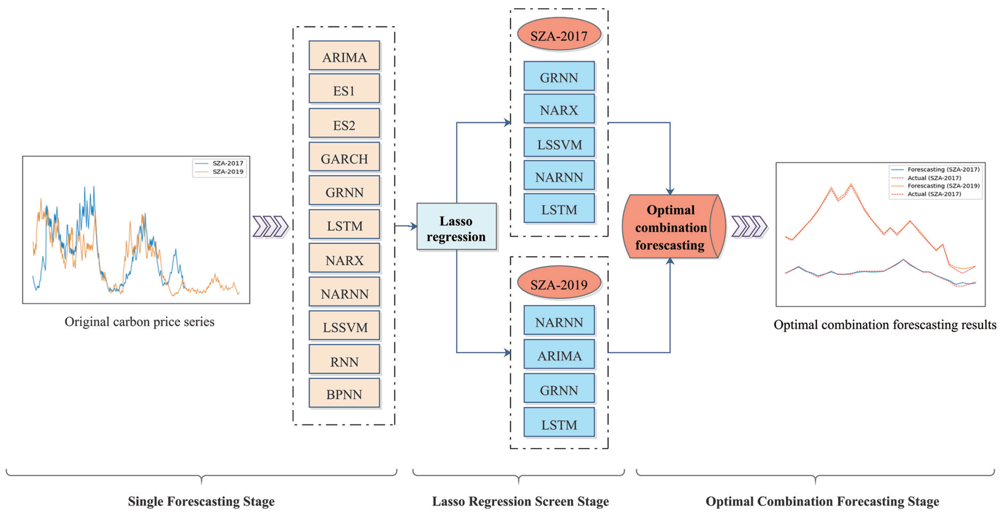
Nevertheless, existing methods for combination forecasting typically use one or a few specific methods. Specifically, various forecasting methods can provide practical information for carbon price forecasting from different perspectives due to the varying model settings. This study combines various models for carbon price forecasting. Eleven single forecasting models, namely, the autoregressive integrated moving average model (ARIMA), the exponential smoothing prediction method (ES1), Holt’s exponential smoothing prediction method (ES2), the generalized autoregressive conditional heteroscedasticity prediction model (GARCH), the generalized regression neural network prediction model (GRNN), the long short-term memory prediction model (LSTM), the nonlinear autoregression with external input prediction model (NARX), the nonlinear autoregressive neural network prediction model (NARNN), the least square support vector machine prediction model (LSSVM), the recurrent neural network model (RNN), and the back propagation neural network prediction model (BPNN), are employed to fully exploit the information provided by each method and establish the optimal combination forecasting model based on the least absolute shrinkage and selection operator (Lasso) regression.

The qualitative analysis method is commonly used for the first investigation of carbon price forecasting [7]. With the swift progress of statistics and economics, as well as the rapid penetration of machine learning technology, researchers are gradually exploring more accurate methods to capture the evolution of carbon price series. In general, the current research on carbon price forecasting is slowly shifting focus from single forecasting methods to hybrid forecasting methods.

Specifically, the single prediction method mainly refers to classical measurement and excellent artificial intelligence models. The former is based on a traditional econometric model to predict the time series. For instance, ARIMA, the most traditional time series prediction model, was used to forecast the linear components of the European Union’s carbon pricing series with favorable performance [8]. In addition, based on the second-stage carbon price data of the European Climate Exchange (ECX) from 2008 to 2011, GARCH [9,10] was found to have a better fitting degree than the k-nearest neighbor model and implied volatility. Furthermore, the improved ARIMA-GARCH model also made a good prediction of the carbon price fluctuation in the European Union, which effectively captured the skewness and the fluctuation behavior in different stages [11]. To sum up, these models are all based on comprehensive statistics and can make sound predictions for stationary time series under certain assumptions. Notwithstanding, considering the prominent non-stationary and nonlinear features of carbon trading price series, the econometric prediction model cannot capture such elements accurately, so the prediction accuracy needs further improvement. Fortunately, the artificial intelligence model makes up for this defect to some extent.

With the swift advancement of machine learning, a growing number of artificial intelligence models are being used to forecast carbon prices. Compared with the econometric prediction model, these models have more robust adaptability and generalization ability. Furthermore, they can more accurately mine the nonlinear laws between data. The BP neural network, for example, is an artificial neural model that conducts reverse training based on errors, can modify any complexity mapping relationship, and has a strong nonlinear prediction ability [12]. Nevertheless, it is easy for the model to suffer from premature convergence caused by local minima. To solve this problem, Sun and Huang [13] combined the genetic algorithm (GA) with the BP model to further improve the training speed. At the same time, they applied this model to predict carbon price series in three Chinese markets, Beijing, Shanghai, and Hubei. Moreover, the prediction effectiveness of the model was proven using three error indicators. Likewise, LSSVM has also achieved good results in carbon price prediction, the core problem of which is determining the kernel function and the optimal parameters. In comparison to the BP neural network, this model can successfully solve the volatility of training effectiveness. Zhu et al. [14] used empirical mode decomposition (EMD) to improve the LSSVM model’s resilience. In addition, Atsalakis et al. [15] creatively proposed three-carbon price prediction methods: the neuro-fuzzy hybrid controller (NFHC), the adaptive neuro-fuzzy inference system (ANFIS), and the artificial neural system. According to the findings, the second method has the highest forecast accuracy and the largest development potential. However, these artificial intelligence models also have their limitations, for example, that they cannot completely capture various feature information of time series. When the time series fluctuates wildly, this kind of model cannot deliver ideal prediction results.

On the other hand, considering that the single forecasting model has certain limitations and cannot accurately capture the practical characteristics of the carbon price series, the existing carbon price research gradually adopts the combination forecasting method [16]. This method may fully exploit the benefits of each individual prediction model, hence increasing forecast accuracy in particular. Zhu et al. [17] combined LSSVM, GARCH, and EMD to set up a new nonlinear integrated combination forecasting model. Firstly, the carbon price series was decomposed using EMD into a residual value and multiple intrinsic modal functions, which are classified as high-frequency, low-frequency, and trend functions. After this, they considered using the GARCH model to predict the high-frequency function and using the LSSVM model to predict the low-frequency as well as trend functions. Finally, they employed LSSVM to integrate the predicted values. Nevertheless, modal mixing may interfere with EMD decomposition, so functions with the same frequency cannot be accurately decomposed. For this reason, researchers created the variational modal decomposition (VMD) model [18]. By combining this model, modal reconstruction (MR), and the optimal combination forecasting model (CFM), Zhu et al. [19] developed a novel combination forecasting method that increased the carbon price prediction accuracy substantially. In addition, Sun et al. [20] also created a new integrated forecasting model, which combined weighted least squares support vector machine (WLS-SVM), linear particle swarm optimization (LDWPSO), and integrated empirical mode decomposition (EEMD). Moreover, they apply it to the empirical research of carbon trading markets in Hubei, Guangdong, and Shanghai. Similarly, by combining fractal Brownian motion (FBM) with GARCH, Liu et al. [21] successfully predicted the carbon trading price of the European Energy Exchange (EUA).

After carefully analyzing the current carbon price combination forecasting models, we can see that each individual prediction method can extract sufficient information from various perspectives. Nonetheless, the accuracy of each method’s forecast varies over time. That is, the “high and low” condition emerges. Consequently, combined forecasting can incorporate the benefits of each forecasting method while also improving model forecasting accuracy. However, because there are a host of single prediction methods, some of them supply repeated information, increasing prediction error and computational complexity if they are all utilized together. As a result, one of the significant difficulties in this study is effectively picking suitable approaches among the single prediction models for combination.

Generally, linear and nonlinear algorithms are the most common data dimensionality reduction techniques. Researchers studied linear dimension reduction methods such as principal component analysis (PCA), independent component analysis (ICA), and factor analysis (FA) in the early research [22,23,24]. These methods, based on feature extraction, translate data from a high-dimensional to a low-dimensional space and use the extracted variables to represent the original whole. Furthermore, scholars are gradually adopting nonlinear dimensionality reduction approaches such as isometric mapping (Isomap), kernel-based principle component analysis (KPCA), and stochastic neighborhood embedding (SNE) [25,26,27] as data structures become more complicated. KPCA is a PCA-based method for improving nonlinear data processing [28]. Simultaneously, SNE is a fantastic learning tool with excellent visualization functions. Laurens et al. [29] devised the t-SNE model on this foundation. The algorithm pays more attention to the correlation between neighboring sample points to better demonstrate the nonlinear relationship between variables. While these solutions can be used for a wide range of problems, they do have some limitations. Other issues, such as the selection of sample size, inability to detect outliers, and estimation of intrinsic dimensionality, have not been addressed. Considering the nonlinearity of carbon pricing data and the possibility of multiple co-linearities in a single forecasting model, we chose to eliminate collinearity statistically. In particular, the Lasso regression model is used to reduce the data dimensionality.

The Lasso regression model, on the other hand, has become a popular linear regression model in recent years [30], which is widely used in computer science, biomedicine, engineering, and other fields [31,32,33,34]. The essence of this model is a kind of compressed estimation. By constructing a penalty function, the sum of absolute values of regression coefficients is less than a specific constant. Meanwhile, the sum of residual squares is minimized so that some coefficients are selected as 0. Finally, the coefficients of each explanatory variable are determined. Furthermore, scholars have gradually introduced the Lasso regression model into economics research. For example, Anuja et al. [35] explored which factor is the key to becoming an influencer on social platforms with this method. Theodore et al. [36] used the Lasso regression model to analyze bitcoin income. They concluded that both the gold return rate and search intensity have the most significant impact on the bitcoin return rate. Similarly, Liu et al. [37] used the Lasso method to determine the variables affecting the efficiency of green innovation in high-tech industries.

Furthermore, Lasso regression models have also begun to be used by current academics to establish the weights of the combined models, thus improving the prediction accuracy. Among these, Diebold et al. [38] propose an approach based on “partial equality LASSO” (peLASSO), which outperforms other models in terms of forecasting results by decreasing the weights of the remaining portfolio weights to the average level and setting some weights to zero. This study was even applied to the European Central Bank Survey of Professional Forecasters, demonstrating its potential for practical application. In addition, Zhang et al. [39] compared the Lasso model with other models, such as ridge regression, principal component regression, and partial least squares in forecasting oil prices. The experimental findings demonstrate the Lasso model’s capacity to choose reliable predictors that add information beyond that offered by rival models. Similar to this, Zhang et al. [40] suggested using a time autocorrelation-based regression model to estimate the concentration of suspended sediment. By using the “shrinkage” effect of the Lasso model, the model was able to identify the most significant factor among the analyzed parameters and compress the contributions of other factors to zero. The results show that the Lasso method is able to obtain prediction results with minimum root mean square error and standard deviation. In conclusion, these studies demonstrate that the use of the Lasso model can increase forecasting accuracy and identify the most crucial predictors, giving decision makers more precise and dependable forecasting findings. In particular, no one has used this method to forecast carbon prices.

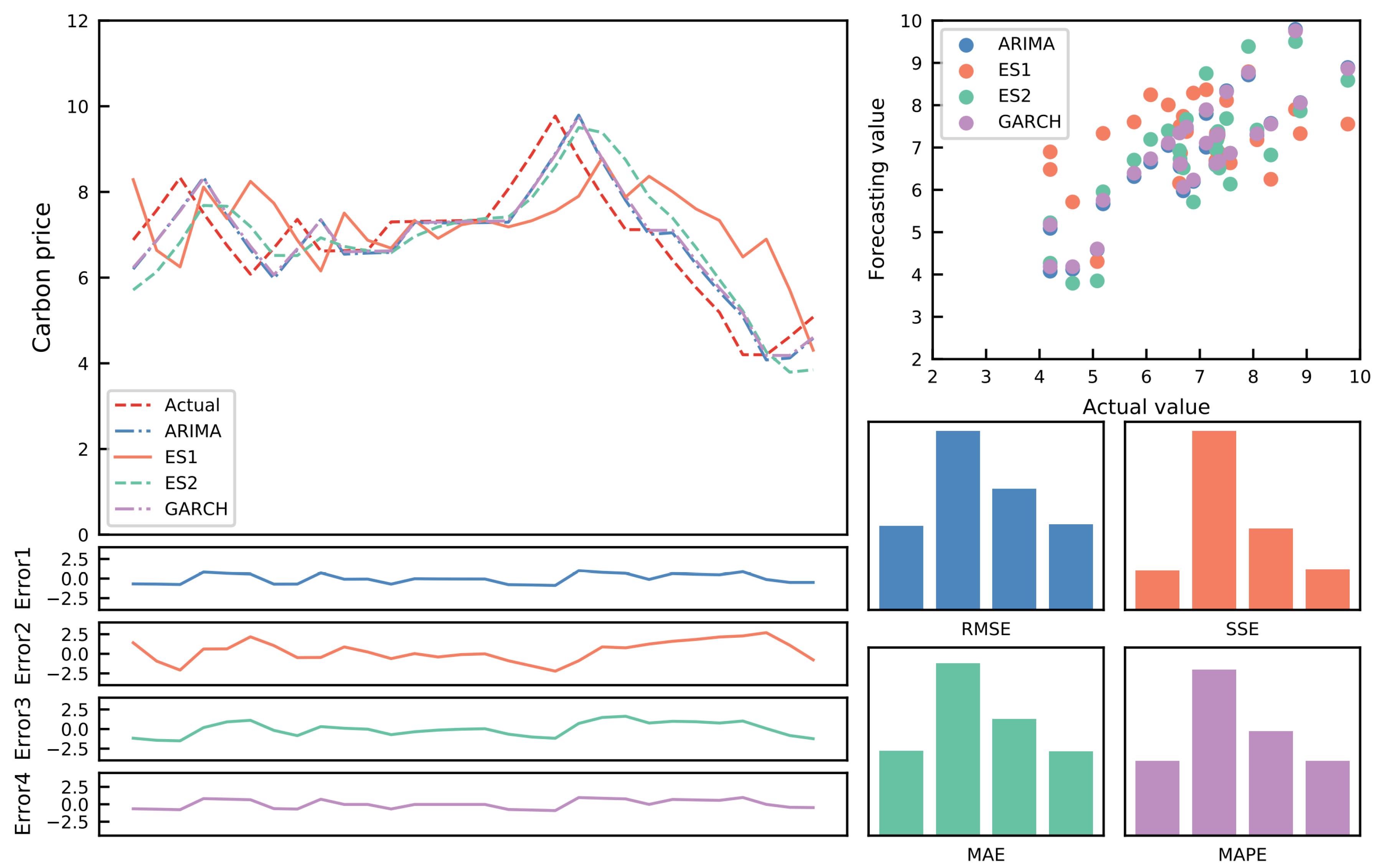
Accordingly, this research presents a Lasso regression-based carbon price combination forecasting model. First, nine well-behaved single prediction models are selected to separately predict the carbon price series. Thus, the initial prediction values are obtained. In addition, the optimal weights of each model can be derived after filtering each model using a Lasso regression-based combined forecasting model. Lastly, the product of the predicted values of each model and the optimal weight is added to obtain the final combined prediction result. In addition, we use the carbon price data of Shenzhen for empirical research and consider four error indicators to corroborate the model’s prediction effectiveness.

This study contributes to the literature in following ways:

(1) For the first time, the Lasso regression model is used to investigate carbon price combination prediction, which partially solved the challenge of calculating the weight of the combination forecast.

(2) Past research on carbon price combination forecasting usually considered three or four single forecasting models. In comparison, eleven excellent single prediction models are selected in this study, which can capitalize on the advantages of different carbon price prediction models and internalize the characteristics of carbon price series more comprehensively, thus improving the prediction accuracy.

The remainder of this research is as follows. Section 2 introduces eleven commonly used single prediction models and Lasso regression models, which lays a solid theoretical foundation for proposing new models later. Then, the combination forecasting model of the carbon price based on Lasso regression is constructed. Additionally, Section 3 describes the data and the evaluation index. Section 4 contains the empirical analysis. Finally, Section 5 elaborates on the study’s primary findings and discusses future research.

2. Methodology

Several excellent single prediction models and Lasso regression models are introduced in this part, laying a solid theoretical foundation for the new model. On the basis of these former models, we establish a carbon price combination forecasting model based on Lasso regression.

2.1. A Meta-Analysis of Carbon Price Portfolio Forecasting Models

This article conducts a meta-analysis of the literature on carbon price forecasting for the years 2000–2023. First, we conducted searches for the terms “carbon price forecasting” and “combination forecasting model” in databases including Google Scholar, Web of Science, and Science Direct. As a result, we found a total of 606 papers. Second, the following criteria were established to further screen the literature, taking into account the needs for a meta-analysis for literature screening and the alignment of the topic with the research direction: excluding literature whose subject matter did not correspond to the research question; keeping only one piece of literature that had a great deal of overlap in the research models and conclusions; and excluding empirical studies, theoretical studies, and review studies that lacked conversion indicators for effect values. Finally, we selected 56 papers for independent coding and conversion into meta-analysis effect values. Specifically, the coding content consisted of the description of the study and the effective value, in order. The former included the name, number, author, year, and journal title of the study, while the latter included the study model, sample size and its related properties, and other effect values. The entire process is shown in Figure 1.

The meta-analysis’s conclusions were reached after a number of analyses, including heterogeneity tests and bias analyses. Initially, we discovered that, among the screened studies on carbon trading price forecasting, the prediction outcomes of the literature using combination forecasting models were significantly superior to those of the literature using single forecasting models. Additionally, for various datasets, each model’s accuracy and prediction outcomes vary, each having benefits of their own. Consequently, it is crucial to choose an appropriate combination of single carbon price forecasting models. At last, we chose 11 single forecasting models from the literature that are relatively well-fitted and appear most frequently in high-quality journals as the basis for the following combination of projections. These models were chosen from a variety of perspectives.

2.2. Several Well-Behaved Single Prediction Models

2.2.1. Exponential Smoothing Prediction Method

This method reduces the influence of distant data on the prediction results by assigning the weight used to converge [41], thus enhancing the prediction accuracy. The first exponential smoothing prediction approach can be utilized with no evident change rule but some correlation in the time series. The basic formula is as follows:

$$S_t^{\left(1\right)}=a·y_t+(1-a)·S_{t-1}^{\left(1\right)}$$

(1)

In this study, $S_t^{\left(1\right)}$ is expressed as the predicted carbon price, $y_t$ denotes the actual carbon price data in the current period, and $S_{t-1}^{\left(1\right)}$ represents past period exponential smoothing values. The smoothing coefficient, a, has a value range of $[0,1]$.

2.2.2. Holt’s Exponential Smoothing Prediction Method

The first exponential smoothing prediction will lag when the time series shows a large linear trend. As a result, Holt’s exponential smoothing prediction is used to correct the variance based on the first exponential smoothing. The formula is as follows:

$$S_t^{\left(2\right)}=a{S}_t^{\left(1\right)}+(1-a)S_{t-1}^{\left(2\right)}$$

(2)

$$\begin{array}{c}{y}_{t+T}^{\prime }=a_t+b_t·T,\left\{\begin{array}{c}{a}_t=2S_t^{\left(1\right)}+S_{t-1}^{\left(2\right)}\hfill \\ b_t=\frac{a}{1-a}\left(S_t^{\left(1\right)}-S_t^{\left(2\right)}\right)\hfill \end{array}\right.\end{array}$$

(3)

where $S_t^{\left(1\right)}$ and $S_t^{\left(2\right)}$ respectively indicate the first and second exponential smoothing prediction values of the t-period carbon price series and $S_{t-1}^{\left(2\right)}$ presents the $t-1$ period carbon pricing series’ second exponential smoothing prediction result. In addition, $y_{t+T}^{\prime }$ denotes the $t+T$ period prediction value, T means the number of periods from the first to the second prediction period, and $a_t$ and $b_t$ are intercept and slope, respectively.

2.2.3. Generalized Autoregressive Conditional Heteroscedasticity Prediction Model (GARCH)

GARCH is an extended form of the ARCH model that is widely used to predict and analyze the volatility of financial time series [42]. The following is the specific calculating formula:

$$y_t=x_t\theta +{\epsilon }_t,{\epsilon }_t\sim N\left(0,{\sigma }_t^2\right)$$

(4)

$${\sigma }_t^2={\alpha }_0+\sum _{i=1}^p{\alpha }_i{u}_{i-t}^2+\sum _{j=1}^q{\beta }_j{\sigma }_{i-j}^2$$

(5)

Formula (4) is the conditional mean equation, where $y_t$ denotes the predicted value of carbon price, $x_t$ means the independent variable, and ${\epsilon }_t$ is the random disturbance term. Meanwhile, Formula (5) shows the conditional variance formula, where p is lag order and q denotes the residual square and lag term number. In addition, both ${\alpha }_i$ and ${\beta }_j$ represent regression coefficients, and $u_i$ is a sequence of independent identically distributed random variables with mean 0 and variance 1.

To meet the positive variance and ensure the stability of the model, the following conditions should be met: ${\alpha }_0>0,{\alpha }_i\ge 0,{\beta }_i\ge 0,{\sum }_{j=1}^p{\beta }_j+{\sum }_{i=1}^p{\alpha }_i<1$.

2.2.4. Autoregressive Integrated Moving Average Prediction Model (ARIMA)

ARIMA is a classical time series model proposed by Box–Jenkins [43], widely used to predict various time series. Assume that the variance of the disturbance terms is constant and the residual series are independent of each other. The formula is expressed as follows:

$${\omega }_t=c+{\Phi }_1{\omega }_{t-1}+\cdots +{\Phi }_p{\omega }_{t-p}+{\epsilon }_t+{\theta }_1{\epsilon }_{t-1}+\cdots +{\theta }_q{\epsilon }_{t-q}$$

(6)

$$\Phi \left(L\right){(1-L)}^d{y}_t=c+\Theta \left(L\right){\epsilon }_t$$

(7)

$$\begin{array}{c}\left\{\begin{array}{c}\Phi \left(L\right)=1-{\Phi }_{1}L-{\Phi }_2{L}^2-\cdots -{\Phi }_p{L}^p\hfill \\ \Theta \left(L\right)=1-{\theta }_{1}L-{\theta }_2{L}^2-\cdots {\theta }_q{L}^q\hfill \\ {\omega }_t={\Delta }^d{y}_t={(1-L)}^d{y}_t\hfill \end{array}\right.\end{array}$$

(8)

In the above formula, $y_t$ represents the carbon price counted at the time t, and ${\omega }_t$ indicates the stationary sequence of $y_t$ after d times of difference. In addition, ${\epsilon }_t$ is the variance, $\mathrm{L}$ is the delayed operator, and q is the moving average model’s order. Moreover, ${\Phi }_1,{\Phi }_2\cdots {\Phi }_p$, as well as ${\theta }_1,{\theta }_2\cdots {\theta }_q$, are unknown parameters to be estimated in the model.

2.2.5. Least Square Support Vector Machine Prediction Model (LSSVM)

LSSVM is an optimized support vector machine (SVM). In this model, equality constraints are used instead of inequality constraints, thus transforming the original problem into solving linear equations, which dramatically improves the learning efficiency [44]. The optimization function is as follows:

$$\left\{\begin{array}{c}\underset{w,m,e}{min}\frac{1}{2}{\parallel \omega \parallel }^2+\frac{1}{2}\lambda \sum _{i=1}^N{e}_i^2\hfill \\ \mathrm{s}.\mathrm{t}.y_i={\omega }^T\psi \left(x_i\right)+m+e_i.i=1,2,\cdots ,N\hfill \end{array}\right.$$

(9)

where $\lambda$ presents the regularization parameter, which directly determines the model’s training error and goodness of fit, and $e_i$ is the error variable. Next, the Lagrange multiplier $a_i$ is introduced to convert the aforementioned function into the Lagrange form:

$$L=\frac{1}{2}{\parallel \omega \parallel }^2+\lambda \frac{1}{2}\sum _{i=1}^N{e}_i^2-\sum _{i=1}^N{a}_i\left({\omega }^T\psi \left(x\right)+m+e_i-y_i\right)$$

(10)

Find the optimal solution of the above formula, and perform partial differentiation on $\omega ,m,e_i,a_i$. After that, eliminating $e_i$ and $\omega$ yields the following linear equations:

$$\left[\begin{array}{cc}0\hfill & R_N^T\hfill \\ R_N\Omega ij+\frac{1}{\lambda }I\hfill \end{array}\right]\left[\begin{array}{c}m\hfill \\ a\hfill \end{array}\right]=\left[\begin{array}{c}0\hfill \\ y\hfill \end{array}\right]$$

(11)

where $\left\{\begin{array}{c}{\Omega }_{ij}=\psi {\left(x_i\right)}^T\psi \left(x_i\right)=h\left(x_i,x_j\right)(i,j=1,2,\cdots ,N)\hfill \\ R_N={[1,1,\cdots ,1]}^T,a={\left[a_1,a_2,\cdots ,a_N\right]}^T\hfill \end{array}\right.$

The values of a and m can be obtained by solving the above equation, from which the prediction function of LSSVM is derived:

$$\left\{\begin{array}{c}y=\sum _{i=1}^N{a}_{i}H\left(x,x_i\right)+m\hfill \\ H\left(x,x_i\right)=exp\left(-{\left(x_i-x\right)}^2/2{\sigma }^2\right)\hfill \end{array}\right.$$

(12)

2.2.6. Generalized Regression Neural Network Prediction Model (GRNN)

GRNN belongs to the forward propagation network with excellent learning efficiency and nonlinear mapping ability [45]. As a result, it is commonly employed in predicting nonlinear time series. In addition, this model has four layers: input, mode, summation, and output. The image is shown in Figure 2.

The formula of each layer is as follows:

$$\left\{\begin{array}{c}{m}_i=exp\left[-\frac{{\left(X-X_i\right)}^T\left(X-X_i\right)}{2{\xi }^2}\right],i=1,2,3,\cdots n\hfill \\ \sum _{i=1}^n{y}_{i}exp\left[-\frac{{\left(X-X_i\right)}^T\left(X-X_i\right)}{2{\xi }^2}\right];S_{Nj}=y_{ij}{M}_i,j=1,2,\cdots ,k\hfill \end{array}\right.$$

(13)

$$\sum _{i=1}^{n}exp\left[-\frac{{\left(X-X_i\right)}^T\left(X-X_i\right)}{2{\xi }^2}\right];S_D=\sum _{i=1}^n{M}_i$$

(14)

$$y_j=\frac{S_{Nj}}{S_D},j=1,2,\cdots ,k\mid$$

(15)

where $\sigma$ presents the smoothness factor and $X_i$ denotes the learning sample of the ith neuron. Additionally, the connection weight between the ith model layer neuron and the jth summation layer neuron is $y_{ij}$. Moreover, $y_j$ indicates the jth neuron’s output values.

2.2.7. Nonlinear Autoregressive Neural Network Prediction Model (NARNN)

NARNN can be regarded as the nonlinearization of the classical time series prediction model. This model takes effects through the values of the first d times of the t time of the historical series [46]. In addition, the network structure includes the input layer, hidden layer, and output layer. The following is the calculation formula:

$$z\left(t\right)=f\left(z\right(t-1),z(t-2),\cdots ,z(t-d\left)\right)$$

(16)

where ${[z(t-1),z(t-2),\cdots ,z(t-d)]}^T$ denotes the input variable and $z\left(t\right)$ implies the output variable, i.e., the forecast value of the carbon price at t. Meanwhile, d presents the order of the delay signal.

2.2.8. Nonlinear Autoregressive with External Input Prediction Model (NARX)

NARX is an externally input nonlinear autoregressive neural network. Specifically, as a nonlinear system identification tool, NARX can be utilized for nonlinear time series forecasting and real-world problems such as air–gas compression systems and predicting the hysteresis effects of bolted joint structures [47,48]. The image is shown in Figure 3.

The model is described as follows:

$$z(n+1)=f\left[\begin{array}{c}z\left(n\right),\cdots z\left(n-d_z+1\right);v(n-k),v(n-k+1),\\ \cdots ,v\left(n-d_v-k+1\right)\end{array}\right]$$

(17)

where $v\left(n\right)\in R,w\left(n\right)\in R,z\left(n\right)\in R$ represent the input and output in this model at n time points, respectively. In addition, $d_v\ge 1,d_z\ge 1,d_v\le d_z,d_v$ denotes the input-storage order, and $d_z$ indicates the output-storage order. In addition, $k(k\ge 0)$ is a lag term called process time.

2.2.9. Long Short-Term Memory Prediction Model (LSTM)

The LSTM neural network has been widely utilized in dealing with timing problems such as speech recognition and translation since it was established by Hochreiter and Schmidhuber in 1997 [49]. After submitting a new state for linear feedback transfer, the gradient explosion and gradient vanishing problems of recurrent neural networks can be effectively solved. The image is shown in Figure 4.

The expressions of the model are as follows:

$$\left\{\begin{array}{c}{z}_t=\sigma \left(W_f·\left[m_{t-1},x_t\right]+b_f\right)\hfill \\ i_t=\sigma \left(W_i·\left[m_{t-1},x_t\right]+b_c\right)\hfill \\ {\tilde{c}}_t=tanm\left(W^{\left(c\right)}{x}_t+U^{\left(e\right)}{m}_t-1\right)\hfill \\ c_t=z_t\ast c_{t-1}+i_t\ast {\tilde{c}}_t\hfill \\ o_t=\sigma \left(W_0·\left[m_{t-1},x_t\right]+b_0\right)\hfill \\ m_t=o_t\ast tanm\left(c_t\right)\hfill \end{array}\right.$$

(18)

where $x_t$ denotes the current input, $m_{t-1}$ is the hidden state at the last moment, and $x_t$ and $m_{t-1}$ jointly determine the amount of information retained by the LSTM cell state. In addition, $\sigma$ presents the logistic function, $z_t$ indicates the forgetting gate, and $o_t$ is the output gate. Moreover, $W_f$ and $b_f$ are the trainable parameters in the forget gate, ${\tilde{c}}_t$ is the information added to the LSTM cell state, and $c_{+}$ represents the updated LSTM cell state.

2.2.10. Back Propagation Neural Network Prediction Model (BPNN)

The BP neural network model shows good predictive ability in describing nonlinear problems, such as carbon price prediction [49]. Precisely, the basic structure is made up of three layers: input, concealed, and output. The model is described as follows: The output of each unit in the hidden layer and the output layer are:

$$n_i=f\left(H_i\right),i=1,2,\cdots ,n$$

(19)

$$y_i=f\left(O_i\right),i=1,2,\cdots ,l$$

(20)

Calculate the sum of squared errors according to the predicted value and expected output value $d_t$:

$$E=\frac{1}{2}\sum _i{e}_i^2=\frac{1}{2}\sum _{i=1}^l{\left(d_i-y_i\right)}^2$$

(21)

Adjust the connection weight by error:

$$t_{ij}(t+1)=t_{ij}\left(t\right)+\eta (dt-yt)yt(1-yt)ne{t}_j,i=1,2,\cdots l,j=1,2,\cdots n$$

(22)

$$\begin{array}{c}{w}_{ij}(t+1)=w_{ij}\left(t\right)+\eta {\displaystyle \sum _{k=1}}\left(d_k-y_k\right)y_k\left(1-y_k\right)t_{ki}ne{t}_j\left(1-ne{t}_i\right)x_j\\ i=1,2,\cdots n,j=1,2,\cdots m\end{array}$$

(23)

where the implicit and output layer input variables are denoted by $H_i$ and $O_i$. The weight between the output layer and the hidden layer is $w_{ij}$. In addition, the weight between the hidden layer and the output layer equals $t_{ij}$, and the function between the output layer unit and the hidden layer unit is a sigmoid function

2.2.11. Recurrent Neural Network Model (RNN)

The recurrent neural network model (RNN) is a feedforward neural network model that is an upgraded model based on the BP neural network [50]. It effectively solves sequence data learning issues and is frequently used in speech recognition, machine translation, and other domains.

In contrast to the BP neural network model, this model forms connections between itself and neurons, allowing the network to have a memory function. The image is shown in Figure 5.

The formula is as follows:

$$\mathrm{R}=\frac{1}{2}\sum _i{\left(H_i-O_i\right)}^2$$

(24)

$$\begin{array}{c}\Delta W_{ij}^k(n+1)=-\alpha \partial E/\partial W_{ji}+\beta \Delta W_{ij}^k\left(n\right)\\ (k=1,2,\cdots ,K;j=1,2,\cdots ,J)\end{array}$$

(25)

where R denotes the mean square deviation between the actual and expected outputs $O_i$ and $H_i$. What is more, ∂ and $\beta$ represent learning efficiency and momentum factor, respectively. Simultaneously, n denotes the number of iterations, k is the number of inputs, and j indicates the number of neurons in the hidden layer.

2.3. Standard Lasso Regression Model

In general, the least squares regression approach (OLS) can be used to obtain the coefficients of the linear regression model by reducing the sum of squares of errors. However, when the quantity of explanatory variables is too large or partially linearly related, the prediction accuracy of this model is often insufficient and the influence of collinearity cannot be eliminated, so we consider building a Lasso regression model.

The Lasso regression model can not only deal with the issue of collinearity but can also rationalize the coefficients of each explanatory variable more accurately. Its essence is a kind of compressed estimation. By constituting a penalty function, the sum of absolute values of regression coefficients is less than a constant. Moreover, the sum of residual squares is also minimized, so some coefficients are filtered as 0. The specific penalty function is as follows:

$${\widehat{\beta }}_{\mathrm{Lasso}}=arg\underset{\beta \in R^d}{min}\left({\parallel Y-X\beta \parallel }^2+\lambda \sum _{j=1}^d\left|{\beta }_j\right|\right)$$

(26)

The above formula can be rewritten as:

$${\widehat{\beta }}_{\mathrm{Lasso}}=arg\underset{\beta \in R^d}{min}{\parallel Y-X\beta \parallel }^2\mathrm{s}.\mathrm{t}.\sum _{j=1}^d\left|{\beta }_j\right|\le t,t\ge 0$$

(27)

where the second formula is the Lagrange form of the first formula, and t denotes the harmonic parameter. If $t_0={\sum }_{j=1}^d\left|{\widehat{\beta }}_j\left(OLS\right)\right|$, when $t<t_0$, some coefficients of the penalty function will be 0, thus enhancing the model’s prediction performance. On the other hand, as a regularization parameter, $\lambda$ presents the core of the fitting effect. If its value is too large, most of the coefficients may be zero, thus decreasing the forecasting precision of the model. Otherwise, it will lead to over-fitting of the model. In this study, we consider the cross-validation method to select $\lambda$.

2.4. Combination Forecasting Model of Carbon Price Based on Lasso Regression

A combined forecasting model denotes that calculating different weights according to the forecasting values of individual models can obtain the eventual forecasting value [51]. During the whole process, the problem of gaining weight is crucial, which directly determines the prediction effect of the model. Therefore, how to obtain the optimal weight has become an important issue.

This study puts forward a combined forecasting model with the Lasso regression model that solves the dilemma of determining the optimal weight. At the same time, it makes up for the deficiencies in the existing carbon price prediction research. The complicated construction steps are shown under Figure 6:

Step 1: Data preprocessing.

First, fill in the blanks and delete outliers. Subsequently, test the nonlinearity and nonstationarity of the carbon price time series.

Step 2: Calculate the values of eleven single forecasting models.

According to the characteristics of different models, the optimal parameter values can be obtained in advance. After that, to obtain the initial forecast value, eleven single forecast models, such as ARIMA, NARNN, BP, and LSTM, are considered to predict the carbon price series. The prediction result is ${\widehat{x}}_{it},i=1,2,\cdots ,10;t=1,2,\cdots ,T$, which can be understood as the prediction value of the ith method at the t time.

Step 3: Correlation test and Lasso regression screening.

To test the correlation, the correlation coefficient between the expected value of the single forecasting model and the actual value of the carbon price is calculated. The Lasso regression model then selects a portion of the model coefficients as 0 based on the prediction outcomes of the single prediction model. These models will be phased out in the future. Furthermore, the chosen model will be used for the combination prediction to follow.

Step 4: The chosen model is employed for combination prediction.

The weighted average method is an effective way to increase combined forecasting accuracy. This strategy usually gives a constant weight to a single prediction model, but it ignores the fact that the forecast accuracy of each model varies with time. As a result, the induced ordered weighted averaging (IOWA) operator is used in this study, and combined prediction is gained by reducing the sum of error squares. Then, the predictions of various models are reordered at the same time. The modified sequence can then be weight-averaged to achieve the final anticipated value.

Assume that the real value of the carbon price at time t is $x_t$. At the same time, the ith single prediction model’s prediction value $x_{it}$ has a prediction accuracy of $b_{it}$:

$$b_{it}=\left\{\begin{array}{cc}0,\hfill & \left|(x_t-x_{it}\right)/x_t|\ge 1\hfill \\ 1-\left|(x_t-x_{it}\right)/x_t|,\hfill & |\left(x_t-x_{it}\right)/x_t|<1\hfill \end{array}\right.$$

(28)

$$\begin{array}{cc}\hfill & minJ=\sum _{t=1}^T{\mu }_t^2=\sum _{i=1}^m{\omega }_i{\omega }_j\left(\sum _{t=1}^T{\mu }_{it}{\mu }_{jt}\right)\hfill \\ \hfill & \mathrm{s}.\mathrm{t}.\left\{\begin{array}{c}\sum _{i=1}^m{\omega }_i=1\hfill \\ {\omega }_i\ge 0,i=1,2,\cdots ,m\hfill \end{array}\right.\hfill \end{array}$$

(29)

$${\mu }_t=x_t-{\widehat{x}}_t^{\prime }=\sum _{i=1}^m{\omega }_i\left(x_t-x_{b-mdex\left(it\right)}\right)=\sum _{i=1}^m{\omega }_i{\mu }_{it}$$

(30)

where ${\mu }_t$ represents the combined prediction error based on the IOWA operator, ${\mu }_{it}$ denotes the single prediction method error, and ${\omega }_i$ indicates the weight. In addition, the reordered sequence is represented by $x_{b-index\left(it\right)}$. Consequently, we can obtain the ideal weight using this model.

Step 5: Compute the overall predicted value:

$${\widehat{x}}_t^{\prime }=\sum _{i=1}^m{\omega }_i^{\prime }{x}_{b-index\left(it\right)}$$

(31)

3. Data and Evaluation Indicators

3.1. Data Description

Since Shenzhen is one of the earliest pilot cities for carbon emissions trading in China, it has a better market system compared to other cities. Therefore, its carbon emission trading data are more comprehensive and representative. In this study, the Shenzhen SZA-2017 and SZA-2019 carbon price data sets from the CSMAR database are selected as experimental samples. The data range of SZA-2017 is from 31 July 2017 to 9 March 2022, with 427 data samples. The first 397 data sets are used as training sets, while the last 30 samples are used as test sets. The data range of SZA-2019 is from 29 October 2019 to 7 March 2022, with 315 data points. Similarly, the test set consists of the latest 30 samples, while the training set consists of the remaining data. Specifically, training samples are mostly used to determine model parameters and regression coefficients, whereas test samples are primarily used to assess the model’s prediction accuracy. The data set is shown in

Table 1. Description of the datasets.

Datasets	Type	Size	Date Range
SZA-2017	Sample set	427	31 July 2017–9 March 2022
	Training set	397	31 July 2017–28 July 2021
	Test set	30	29 July 2021–9 March 2022
SZA-2019	Sample set	315	29 October 2019–7 March 2022
	Training set	285	29 October 2019–13 December 2021
	Test set	30	14 December 2021–7 March 2022

.

3.2. Forecasting Evaluation

We choose eight metrics to measure the model’s forecasting performance, which are root mean square error (RMSE ), mean absolute percentage error (MAPE), sum of squares error (SSE), mean fundamental error (MAE), Theil U statistic 1 (U1), index of agreement (IA), success ratio (SR), and accuracy. The model’s prediction error is assessed using the first four indices. The stronger the model’s prediction effect, the smaller the values of these four indices are. Similarly, U1 is used to represent the model’s ability to make predictions. The higher the prediction ability, the closer the index value is to 0. On the other hand, IA SR represent the model’s generalization ability, and they are positively correlated with the values. Additionally, the closer the accuracy is to 1, the better the model’s prediction accuracy. The following is the calculating formula:

$$RMSE=\sqrt{\frac{1}{T}\sum _{t=1}^T{\left(x_t-{\widehat{x}}_{it}\right)}^2}$$

(32)

$$SSE=\sum _{t=1}^T{\left(x_t-{\widehat{x}}_{it}\right)}^2$$

(33)

$$MAE=\frac{1}{T}\sum _{t=1}^T|x_t-{\widehat{x}}_{it}|$$

(34)

$$MAPE=\frac{1}{T}\sum _{t=1}^T|\frac{x_t-{\widehat{x}}_{it}}{x_t}|$$

(35)

$$U1=\frac{\sqrt{\frac{1}{T}{\sum }_{t=1}^T{\left(x_t-{\widehat{x}}_{it}\right)}^2}}{\sqrt{\frac{1}{T}{\sum }_{t=1}^T{x}_t^2}+\sqrt{\frac{1}{T}{\sum }_{t=1}^T{\widehat{x}}_{it}^2}}$$

(36)

$$IA=1-\frac{\sqrt{\frac{1}{T}{\sum }_{t=1}^T{\left(x_t-{\widehat{x}}_{it}\right)}^2}}{\sqrt{\frac{1}{T}{\sum }_{t=1}^T{\left(|{\widehat{x}}_{it}-{\overline{x}}_t|+\mid x_t-{\overline{x}}_t|\right)}^2}}$$

(37)

$$\mathrm{Accuracy}=1-\frac{100\%}{T}\sum _{t=1}^T|\frac{x_t-x_{it}}{x_t}|$$

(38)

$$SR=\frac{1}{T}\sum _{t=1}^T{b}_t\times 100\%,b_t=\left\{\begin{array}{c}1,\left({\widehat{x}}_{t+1}-x_t\right)\left(x_{t+1}-x_t\right)\ge 0\hfill \\ 0,\left({\widehat{x}}_{t+1}-x_t\right)\left(x_{t+1}-x_t\right)<0\hfill \end{array}\right.$$

(39)

In addition, the study used the standard DM test [26] to further demonstrate the new model’s prediction advantage in terms of prediction accuracy. Assume that the initial $H_0$ is the two models’ prediction accuracy and is equal. The following are the statistics:

$$H_{dm}=\frac{\overline{o}}{\sqrt{{\widehat{R}}_g/T}};\left\{\begin{array}{c}\overline{o}=\frac{1}{T}\sum _{\mathrm{t}}^T{o}_t,o_t={\left(x_t-x_{m,t}\right)}^2-{\left(x_t-x_{n,t}\right)}^2\hfill \\ {\widehat{R}}_g={\lambda }_0+2\sum _{t=1}^{\infty }{\lambda }_t,\left({\lambda }_t=cov\left(o_{t+1},o_t\right)\right)\hfill \end{array}\right.$$

(40)

The variance of $o_t$ is denoted by ${\lambda }_0$, while the number of observations is represented by T. Moreover, $x_{m,t}$ and $x_{n,t}$ are the two models’ anticipated values for the t period.

4. Empirical Analysis

This section clearly illustrates the proposed model’s prediction outcomes. In addition, the prediction results of other models are presented. Furthermore, eight assessment indices and tests are employed to demonstrate the effectiveness of the new model’s forecast predictions.

4.1. Empirical Results

Figure 7 and Figure 8 show the SZA-2017 prediction results using four classical econometric models and seven artificial intelligence models, respectively. Similarly, the SZA-2019 forecast results are displayed in Figure 9 and Figure 10. The chart shows that the trend of each single forecast model’s forecast series is generally the same as that of the actual series. Nevertheless, the fluctuation ranges in different periods are different. At the same time, the error curve shows that the errors of these models oscillate around 0. It can demonstrate that each model can gather data characteristics from various perspectives and develop its prediction advantages.

In addition, as shown by the scatter plot on the right, the predicted value of each model has a relatively positive linear relationship with the actual value. Furthermore, the convergence degree of the artificial intelligence model is somewhat higher when compared to the traditional measurement model.

Because each model has different predictions of performance over time. Besides, the simple average combination model only takes a simple weighted average of the forecasted values of all individual models and cannot benefit from each model’s prediction benefits. As a result, we first use the Lasso regression model to screen the weights of some models to 0 and then apply the IOWA operator to build the optimal combination prediction model, thus obtaining the optimal prediction value.

The screening results of the Lasso regression model are shown in

Table 2. Description of the data sets.

Data Sets	Benchmark Model
	ARIMA	ES1	ES2	GARCH	BPNNF
SZA-2017	0	0	0	0	0
SZA-2019	0.02	0	0	0	0
	GRNN	LSTM	NARX	NARNN	LSSVM	RNN
SZA-2017	0.2383	0.3506	0.0812	0.0544	0.4321	0
SZA-2019	0.764	0.1507	0	0.0189	0	0

. It can be observed that almost all of the selected models are AI models. At the same time, the weights assigned to each model are different for distinct data sets, indicating that the training effects of models for different feature sequences are heterogeneous. In addition, Figure 11 and Figure 12 exhibit the prediction results of the simple average prediction model and the proposed model for two different data sets. The prediction series of the constituted model is closer to the actual value than the simple average model, with more stable error fluctuations and stronger correlation.

4.2. Forecasting Effectiveness

4.2.1. Prediction Evaluation

This study examines eight evaluation indicators using the SZA-2017 and SZA-2019 data sets as examples.

Table 3. Forecasting performance comparisons of classical measurement models.

Data Sets	Algorithms	Evaluation Criteria
		RMSE	SSE	MAE	MAPE	UI	IA	Accuracy	SR
SZA-2017	ARIMA	0.6194	11.5107	0.539	0.0795	0.0442	0.9027	0.9205	0.4483
	ES1	1.3184	52.1434	1.0977	0.1762	0.0922	0.676	0.8238	0.5172
	ES2	0.8903	23.7781	0.7431	0.1108	0.0634	0.8628	0.8892	0.3103
	GARCH	0.6294	11.8839	0.536	0.0791	0.0448	0.8991	0.9209	0.4483
SZA-2019	ARIMA	1.7926	96.3997	1.6175	0.1084	0.0532	0.981	0.8916	0.3793
	ES1	4.1694	521.5287	3.6116	0.2593	0.1254	0.9335	0.7407	0.4138
	ES2	2.224	148.3787	1.8649	0.1267	0.0651	0.9792	0.8733	0.5172
	GARCH	2.2891	157.2005	1.5438	0.1119	0.0678	0.9792	0.8881	0.5862

,

Table 4. Forecasting performance comparisons of artificial intelligence models.

Data Sets	Algorithms	Evaluation Criteria
		RMSE	SSE	MAE	MAPE	UI	IA	Accuracy	SR
SZA-2017	BPNNF	0.6981	14.6202	0.5663	0.0865	0.0498	0.8768	0.9135	0.5862
	GRNN	0.9633	27.8411	0.7014	0.1254	0.0668	0.7287	0.8746	0.8276
	LSTM	0.4586	6.3087	0.3741	0.0603	0.0322	0.9349	0.9397	0.8621
	NARX	1.4983	67.3485	1.2305	0.1876	0.0984	0.8273	0.8124	0.8621
	NARNN	0.6013	10.8466	0.5142	0.0756	0.0431	0.8888	0.9244	0.4828
	LSSVM	0.5198	8.1066	0.4838	0.0744	0.0381	0.9116	0.9256	0.7931
	RNN	1.0877	35.4897	0.9128	0.137	0.077	0.8295	0.863	0.3793
SZA-2019	BPNNF	2.1472	138.3081	1.4842	0.0979	0.0626	0.9798	0.9021	0.6552
	GRNN	0.968	28.1109	0.8753	0.0528	0.0281	0.9912	0.9472	0.9655
	LSTM	2.0836	130.2406	1.7657	0.1225	0.0647	0.9767	0.8775	0.6897
	NARX	2.0892	130.9463	1.6523	0.1183	0.0606	0.9811	0.8817	0.4828
	NARNN	2.0149	121.7979	1.5881	0.1152	0.0583	0.979	0.8848	0.7241
	LSSVM	2.7319	223.9011	2.3501	0.1476	0.0814	0.9773	0.8524	0.7586
	RNN	2.908	253.7017	2.3475	0.1654	0.0846	0.9686	0.8346	0.3793

and

Table 5. Forecasting performance comparisons of combined forecasting models.

Data Sets	Algorithms	Evaluation Criteria
		RMSE	SSE	MAE	MAPE	UI	IA	Accuracy	SR
SZA-2017	CF	0.5543	9.2173	0.4586	0.0723	0.0391	0.8958	0.9277	0.7931
	BCF	0.2011	1.2128	0.1417	0.0242	0.0143	0.9674	0.9758	0.8621
SZA-2019	CF	1.23	45.3865	1.0285	0.0727	0.0364	0.987	0.9273	0.8966
	BCF	0.3426	3.521	0.2842	0.0214	0.0102	0.9966	0.9786	0.8966

show the eight evaluation index values of all models. By analyzing the contents of the table, the following conclusions can be drawn:

(1) The model substituted in this study has a good prediction performance. The four error indicators of SZA-2017 are 0.2011, 1.2128, 0.1417, and 0.0242, and it has a U1 value of 0.0143. These results are significantly smaller than other benchmark models. In addition, the SZA-2019 results are similar. In addition, considering the model’s generalization ability and prediction efficacy, the model’s IA, SR, and accuracy values are ideal, with 0.9674, 0.8621, and 0.9758, respectively, which are higher than other models. For SZA-2019, all other values are the best except SR (second only to GRNN). As a result, the proposed model has proven to be capable of accurate predictions.

(2) The Lasso regression model provides a robust model screening capacity for carbon price prediction. In this study, the Lasso regression model gives LSTM and LSSVM a heavier weight in SZA-2017, which corresponds to their prediction accuracy in this data set. The error indices of the LSTM model in SZA-2017 are 0.4586, 6.3087, and 0.3741 and a U1 value of 0.0322, which are superior than other single prediction models. At the same time, its IA, SR, and accuracy values provide a significant benefit, indicating that it has improved generalization and prediction effectiveness. Furthermore, all of LSSVM’s index values are close to ideal. Likewise, the SZA-2019 analysis results lead to a similar conclusion. As a result, the Lasso regression model is helpful in further improving the constructed model’s forecasting accuracy.

(3) The simple combination model outperforms most single prediction models in terms of accuracy. The simple combination prediction model’s prediction errors in SZA-2017 are 0.5543, 9.2173, 0.4586, 0.0723, and it has a U1 value of 0.0391. These values are much lower than the four traditional measurement models. It is, however, not superior to all artificial intelligence models. The values of the other three indices are 0.8958, 0.9277, and 0.7931, which are higher than traditional econometric models but lower than some AI models. Likewise, this finding can also be reached by looking at the SZA-2019 index value. Specifically, the underlying reason for this is that the basic average combination model weights all models equally and ignores the differences in prediction between models for various sequences, resulting in information redundancy or over-fitting, thus diminishing prediction ability to some extent.

(4) The prediction outcomes of artificial intelligence models and conventional econometric models both have their own benefits for various data sets. It is discovered that artificial intelligence models do not always perform better than conventional econometric models, and for various data sets, the metrics for each model’s accuracy, reliability, and generalizability of prediction findings fluctuate correspondingly. For instance, the RMSE of ARIMA is lower than that of BPNN, GRNN, NARX, and RNN for the SZA-2017 training set.

4.2.2. Diebold–Mariano Test

The DM test is used to confirm the model’s prediction validity from a statistical standpoint.

Table 6. DM test results of classical measurement models (SZA-2017).

Target Model	Benchmark Model
	ARIMA	ES1	ES2	GARCH
ES1	−2.5585
	(−0.0105)
ES2	−2.4201	1.9856
	(−0.0155)	(−0.0471)
GARCH	−0.8166	2.5907	2.4989
	(−0.4142)	(−0.0096)	(−0.0125)
BPNNF	−1.0812	2.8282	1.6498	−1.0319
	(−0.2796)	(−0.0047)	(−0.099)	(−0.3021)
GRNN	−0.8901	2.3232	−0.2176	−0.8775
	(−0.3734)	(−0.0202)	(−0.8278)	(−0.3802)
LSTM	2.2642	2.9362	2.7597	2.3455
	(−0.0236)	(−0.0033)	(−0.0058)	(−0.019)
NARX	−4.6137	−0.5795	−2.5262	−4.3927
	(0.0000)	(−0.5622)	(−0.0115)	(0.0000)
NARNN	0.6281	2.629	2.2552	0.9081
	(−0.5300)	(−0.0086)	(−0.0241)	(−0.3638)
LSSVM	1.1887	2.6731	2.2178	1.2595
	(−0.2346)	(−0.0075)	(−0.0241)	(−0.2078)
RNN	−3.1842	1.1200	−3.1388	−3.2636
	(−0.0015)	(−0.2628)	(−0.0017)	(−0.0011)
CF	0.8795	3.0642	2.6265	1.1328
	(−0.3791)	(−0.0022)	(−0.0086)	(−0.2573)
BCF	4.0330	3.1914	3.3407	4.0210
	(0.0000)	(−0.0014)	(−0.0008)	(0.0000)

,

Table 7. DM test results of artificial intelligence models (SZA-2017).

Target Model	Benchmark Model
	BPNNF	GRNN	LSTM	NARX	NARNN	LSSVM	RNN	CF
GRNN	−0.8617
	(−0.3889)
LSTM	4.0634	1.2639
	0	(−0.2063)
NARX	−3.832	−1.5408	−4.6798
	(−0.0001)	(−0.1234)	0
NARNN	1.4343	0.9497	−1.9523	4.9468
	(−0.1515)	(−0.3422)	(−0.0509)	0
LSSVM	1.9459	1.1169	−1.8419	4.9589	1.0532
	(−0.0517)	(−0.264)	(−0.0655)	0	(−0.2923)
RNN	−2.497	−0.3708	−3.2872	1.5905	−2.9544	−2.8017
	(−0.0125)	(−0.7108)	(−0.001)	(−0.1117)	(−0.0031)	(−0.0051)
CF	5.1172	1.1438	−1.6489	4.1255	0.6716	−0.4031	3.2632
	0	(−0.2527)	(−0.0991)	0	(−0.5018)	(−0.6868)	(−0.0011)
BCF	5.1286	1.5449	5.8156	5.5011	4.5527	11.7087	3.6188	3.5456
	0	(−0.1224)	0	0	0	0	(−0.0003)	(−0.0003)

,

Table 8. DM test results of classical measurement models (SZA-2019).

Target Model	Benchmark Model
	ARIMA	ES1	ES2	GARCH
ES1	−3.5328
	(−0.0004)
ES2	−1.1555	2.6692
	(−0.2479)	(−0.0076)
GARCH	−1.8358	2.9297	−0.1515
	(−0.0664)	(−0.0034)	(−0.8796)
BPNNF	−0.712	2.5921	0.5064	−1.0319
	(−0.4764)	(−0.0095)	(−0.6126)	(−0.3021)
GRNN	4.0562	3.7633	2.5085	−0.8775
	0	(−0.0002)	(−0.0121)	(−0.3802)
LSTM	−1.1042	2.8376	0.5021	2.3454
	(−0.2695)	(−0.0045)	(−0.6156)	(−0.019)
NARX	−1.4491	2.9907	0.4693	−4.3927
	(−0.1473)	(−0.0028)	(−0.6389)	0
NARNN	−1.131	3.378	0.5061	0.9081
	(−0.2581)	(−0.0007)	(−0.6128)	(−0.3638)
LSSVM	−3.1095	2.6283	−0.9402	1.2595
	(−0.0019)	(−0.0086)	(−0.3471)	(−0.2078)
RNN	−2.4718	1.9124	−3.7775	−3.2636
	(−0.0134)	(−0.0558)	(−0.0002)	(−0.0011)
CF	6.3891	3.7545	2.2895	1.1328
	0	(−0.0002)	(−0.0221)	(−0.2573)
BCF	7.1292	3.9925	2.9186	4.021
	0	0	(−0.0035)	0

and

Table 9. DM test results of artificial intelligence models (SZA-2019).

Target Model	Benchmark Model
	BPNNF	GRNN	LSTM	NARX	NARNN	LSSVM	RNN	CF
GRNN	1.771
	(−0.0766)
LSTM	0.176	1.2639
	(−0.8603)	(−0.2063)
NARX	0.1416	−1.5408	−4.6798
	(−0.8874)	(−0.1234)	0
NARNN	0.2353	0.9497	−1.9523	4.9468
	(−0.814)	(−0.3422)	(−0.0509)	0
LSSVM	−0.9231	1.1169	−1.8419	4.9589	−2.066
	(−0.3559)	(−0.264)	(−0.0655)	0	(−0.0388)
RNN	−4.6763	−0.3708	−3.2872	1.5905	−1.9493	−2.8017
	0	(−0.7108)	(−0.001)	(−0.1117)	(−0.0513)	(−0.0051)
CF	1.5538	1.1438	−1.6489	4.1255	4.5712	−0.4031	3.2802
	(−0.1202)	(−0.2527)	(−0.0992)	0	0	(−0.6868)	(−0.001)
BCF	2.0866	1.544	5.8156	5.5011	6.1023	11.7087	3.5487	4.5468
	(−0.037)	(−0.1224)	0	0	0	0	(−0.0004)	0

provide the inspection’s findings, where the above models are utilized as benchmark models for inspection. We can summarize the tables’ contents as follows:

(1) The prediction accuracy of the model proposed in this study is better than all other models selected when taking into account the findings of the DM test together with the predictive validity results in the preceding section. First of all, when compared to the conventional econometric prediction models, the model created for this study consistently rejected the original hypothesis at the 1% significance level. Therefore, the model performs better than each of the selected econometric models. In addition, the proposed model outperforms other artificial intelligence models relative to the benchmark AI model, except for GRNN, at the 1% or 5% significance level of predictive accuracy. Nevertheless, the proposed new model outperforms the GRNN model in terms of the eight criteria that were previously proposed to gauge the model’s predictive performance. Therefore, the investigation came to the conclusion that the new model outperforms all of the selected artificial intelligence models in terms of prediction accuracy. Furthermore, the prediction accuracy of the model created in this study was significantly better than the simple average combination model at the 1% level, with DM statistics of 3.5456 and 4.5468 for SZA-2017 and SZA-2019, respectively, indicating the importance of the study’s use of the Lasso model to select the optimal weights.

(2) Each type of single forecasting model has its benefits, while their prediction accuracy varies across different training sets. For instance, when using ARIMA as the baseline model to fit predictions to the SZA-2017 data, we discovered that at the 1% or 5% level, this model greatly outperformed the exponential smoothing prediction method, Holt’s exponential smoothing prediction method, NARX, and RNN. Their respective DM scores were −2.5585, −2.4201, −4.6137, and −3.1842. Nevertheless, when the model was used to analyze SZA-2019, the outcomes drastically varied. When other individual models are used as benchmark models, the following pattern can be seen: the Holt’s exponential smoothing prediction method, LSTM, and NARX are no longer significantly less accurate than ARIMA, whereas the exponential smoothing prediction method, GARCH, LSSVM, and RNNN are all significantly less accurate than ARIMA. It is clear that each forecasting model has a unique forecasting advantage due to its ability to capture the pertinent data in the carbon trading price series from various angles.

(3) The simple average combination model’s forecast accuracy was not always higher than that of the other single prediction models. According to the DM test findings, the prediction accuracy of the simple average combination model did not significantly exceed ARIMA, GRNN, NARNN, and LSSVM for the SZA-2017 training set and was even significantly lower than that of the LSTM model. In contrast, when SZA-2019 was used as the training set, the simple average combination model’s DM results at the 1% or 5% level outperformed those of ARIMA, the exponential smoothing prediction method, Holt’s exponential smoothing prediction method, NARX, NARNN, and RNN. This conclusion might be a result of the simple average combination model giving each single model the same weight while ignoring the interactions between the models and their suitability for the training dataset.

5. Conclusions and Discussion

Forecasting an accurate carbon price trend is crucial for the growth of the carbon emission trading market. Given the current carbon price forecasting constraints, an optimal combination carbon price forecasting model based on the Lasso regression model is developed. First, 11 single forecasting models are chosen to forecast the relevant data sets. After that, the Lasso regression model is employed to reduce the dimensionality. Thus, the weights of some models are set to 0. Moreover, the best combination prediction model based on the IOWA operator is used to forecast the remaining models. As a result, the optimal weight can be calculated to obtain the final prediction value. In addition, using the Shenzhen SZA-2017 and SZA-2019 data sets as samples, eight evaluation indices and the DM test are applied to assess the model’s prediction effectiveness from various perspectives. The following breakthroughs and strengths of this paradigm have been identified through empirical and extensive analysis:

(1) Compared to existing benchmark models, the suggested model outperforms them in terms of prediction accuracy, generalization ability, and effectiveness. It introduces a novel strategy for predicting carbon prices.

(2) For the first time, the Lasso regression model is used in carbon price prediction, resolving the challenge of selecting a single prediction model in a combination prediction model.

(3) The simple average combination model’s suboptimal properties are empirically tested, and then the ideal weight is established.

In addition, the study also has some academic significance and practical benefits. On the one hand, the study builds a combined model for predicting carbon trading prices based on Lasso regression and optimal integration, as well as forecasts two different types of carbon trading prices in the Shenzhen carbon trading market, enhancing theoretical research on carbon trading price forecasting and the carbon trading market while also furthering forecasting results and their accuracy. Nevertheless, this study has significant practical implications for the policy making of government agencies, the strategic positioning of emission control businesses, and the decision making of investors. First and foremost, since China’s carbon trading market is currently in a stage of gradual improvement, the accurate price prediction of carbon trading is conducive to a deeper exploration of the intricate patterns of carbon trading prices, providing a reference for government departments to formulate policies related to the carbon trading market and accelerating the establishment of an effective and complete carbon price trading system, further improving the market regulatory mechanism. The study will also assist emission control businesses in predicting the trajectory of carbon trading prices and allocating resources more sensibly and effectively to cut costs and achieve sustainable development. The study can also give investors market information estimates, which can result in more useful investment and financing guidance, given that carbon emission rights are also a financial asset.

Nevertheless, there are still certain restrictions that need to be addressed. First, all of the forecasts in this research are based on historical carbon price data but do not take into account unstructured data, causing the prediction results to lag. More research is needed to determine how to mix this type of data with the combined forecasting model. Furthermore, the combination prediction model used combines traditional measurement methods with artificial intelligence methodologies. However, the decomposition and integration models are not taken into account. As a result, in the future, it may be essential to combine these methodologies with the optimal combination forecasting model to create a more general and robust forecasting model. Ultimately, to optimize its utility, the suggested model can be applied to the prediction of business cycles, economic growth, policy formulation, stock price forecasting, and other relevant domains.

References

1. Wang, P.; Liu, J.; Tao, Z.; Chen, H. Carbon price combination forecasting approach based on multi-source information fusion and hybrid multi-scale decomposition. Eng. Appl. Artif. Intell. 2022, 114, 105172. [Google Scholar] [CrossRef]
2. Tobin, P.; Schmidt, N.M.; Tosun, J.; Burns, C. Mapping states’ Paris climate pledges: Analysing targets and groups at COP 21. Glob. Environ. Chang. 2018, 48, 11–21. [Google Scholar] [CrossRef]
3. Zhou, F.; Huang, Z.; Zhang, C. Carbon price forecasting based on CEEMDAN and LSTM. Appl. Energy 2022, 311, 118601. [Google Scholar] [CrossRef]
4. Huang, Y.; Dai, X.; Wang, Q.; Zhou, D. A hybrid model for carbon price forecasting using GARCH and long short-term memory network. Appl. Energy 2021, 285, 116485. [Google Scholar] [CrossRef]
5. Lu, H.; Ma, X.; Huang, K.; Azimi, M. Carbon trading volume and price forecasting in China using multiple machine learning models. J. Clean. Prod. 2020, 249, 119386. [Google Scholar] [CrossRef]
6. Hao, Y.; Tian, C. A hybrid framework for carbon trading price forecasting: The role of multiple influence factor. J. Clean. Prod. 2020, 262, 120378. [Google Scholar] [CrossRef]
7. Paltsev, S.; Reilly, J.M. An analysis of the European emission trading scheme. In Joint Program Report Series Report 127; MIT: Cambridge, MA, USA, 2005. [Google Scholar]
8. Zhu, B.; Wei, Y. Carbon price forecasting with a novel hybrid ARIMA and least squares support vector machines methodology. Omega 2013, 41, 517–524. [Google Scholar] [CrossRef]
9. Zhou, J.; Huo, X.; Xu, X.; Li, Y. Forecasting the Carbon Price Using Extreme-Point Symmetric Mode Decomposition and Extreme Learning Machine Optimized by the Grey Wolf Optimizer Algorithm. Energies 2019, 12, 950. [Google Scholar] [CrossRef] [Green Version]
10. Byun, S.J. Forecasting carbon futures volatility using GARCH models with energy volatilities. Energy Econ. 2013, 40, 207–221. [Google Scholar] [CrossRef]
11. Chevallier, J. Volatility forecasting of carbon prices using factor models. Econ. Bull. 2010, 30, 1642–1660. [Google Scholar]
12. Han, M.; Ding, L.; Zhao, X. Forecasting carbon prices in the Shenzhen market, China: The role of mixed-frequency factors. Energy 2019, 171, 69–76. [Google Scholar] [CrossRef]
13. Sun, W.; Huang, C. A carbon price prediction model based on secondary decomposition algorithm and optimized back propagation neural network. J. Clean. Prod. 2020, 243, 118671. [Google Scholar] [CrossRef]
14. Zhu, B.; Han, D.; Wang, P.; Wu, Z.; Zhang, T.; Wei, Y.-M. Forecasting carbon price using empirical mode decomposition and evolutionary least squares support vector regression. Appl. Energy 2017, 191, 521–530. [Google Scholar] [CrossRef] [Green Version]
15. Atsalakis, G.S. Using computational intelligence to forecast carbon prices. Appl. Soft Comput. 2016, 43, 107–116. [Google Scholar] [CrossRef]
16. Yang, Y.; Guo, H.; Jin, Y.; Song, A. An Ensemble Prediction System Based on Artificial Neural Networks and Deep Learning Methods for Deterministic and Probabilistic Carbon Price Forecasting. Appl. Soft Comput. 2021, 9, 740093. [Google Scholar] [CrossRef]
17. Zhu, B.; Ye, S.; Wang, P.; He, K.; Zhang, T.; Wei, Y.-M. A novel multiscale nonlinear ensemble leaning paradigm for carbon price forecasting. Energy Econ. 2018, 70, 143–157. [Google Scholar] [CrossRef]
18. Dragomiretskiy, K.; Zosso, D. Variational Mode Decomposition. IEEE Trans. Signal Process. 2014, 62, 531–544. [Google Scholar] [CrossRef]
19. Zhu, J.; Wu, P.; Chen, H.; Liu, J.; Zhou, L. Carbon price forecasting with variational mode decomposition and optimal combined model. Phys. A Stat. Mech. Appl. 2019, 519, 140–158. [Google Scholar] [CrossRef]
20. Sun, W.; Xu, C. Carbon price prediction based on modified wavelet least square support vector machine. Sci. Total Environ. 2021, 754, 142052. [Google Scholar] [CrossRef]
21. Liu, Z.; Huang, S. Carbon option price forecasting based on modified fractional Brownian motion optimized by GARCH model in carbon emission trading. N. Am. J. Econ. Financ. 2021, 55, 1062–9408. [Google Scholar] [CrossRef]
22. Harman, H.H. Modern Factor Analysis; University of Chicago Press: Chicago, IL, USA, 1960. [Google Scholar]
23. Lever, J.; Krzywinski, M.; Altman, N. Principal component analysis. Nat. Methods 2017, 14, 641–642. [Google Scholar] [CrossRef] [Green Version]
24. Diebold, F.; Mariano, R. Comparing Predictive Accuracy. Bus. Econ. Stat. 1995, 13, 253–263. [Google Scholar]
25. Tenenbaum, J.B.; de Silva, V.; Langford, J.C. A global geometric framework for nonlinear dimensionality reduction. Science 2000, 290, 2319–2323. [Google Scholar] [CrossRef] [PubMed]
26. Hoffmann, H. Kernel PCA for novelty detection. Pattern Recognit. 2007, 40, 863–874. [Google Scholar] [CrossRef]
27. Hinton, G.H.; Roweis, S. Advances in neural information processing systems. Stoch. Neighbor Embed. 2003, 15, 833–840. [Google Scholar]
28. Mika, S.; Schölkopf, B.; Smola, A.; Müller, K.R.; Scholz, M.; Rätsch, G. Kernel PCA and de-noising in feature spaces. Adv. Neural Inf. Process. Syst. 1999, 11, 537–542. [Google Scholar]
29. Van der Maaten, L.; Hinton, G. Visualizing Data using t-SNE. J. Mach. Learn. Res. 2008, 9, 2579–2605. [Google Scholar]
30. Tibshirani, R. Regression shrinkage and selection via the lasso: A retrospective Series B Statistical methodology. J. R. Stat. Soc. Ser. Stat. Methodol. 2011, 73, 273–282. [Google Scholar] [CrossRef]
31. Zhao, Z.; Wu, S.; Qiao, B.; Wang, S.; Chen, X. Enhanced Sparse Period-Group Lasso for Bearing Fault Diagnosis. IEEE Trans. Ind. Electron. 2019, 66, 2143–2153. [Google Scholar] [CrossRef]
32. Li, Z.; Jiang, S.; Li, L.; Li, Y. Building sparse models for traffic flow prediction: An empirical comparison between statistical heuristics and geometric heuristics for Bayesian network approaches. Transp. Transp. Dyn. 2017, 7, 107–123. [Google Scholar] [CrossRef]
33. Li, Y.; Wu, F.X.; Ngom, A. A review on machine learning principles for multi-view biological data integration. Brief Bioinform 2018, 19, 325–340. [Google Scholar] [CrossRef] [Green Version]
34. Huang, Y.Q.; Liang, C.H.; He, L.; Tian, J.; Liang, C.S.; Chen, X.; Ma, Z.L.; Liu, Z.Y. Development and Validation of a Radiomics Nomogram for Preoperative Prediction of Lymph Node Metastasis in Colorectal Cancer. J. Clin. Oncol. 2016, 34, 2157–2164. [Google Scholar] [CrossRef] [PubMed]
35. Arora, A.; Bansal, S.; Kandpal, C.; Aswani, R.; Dwivedi, Y. Measuring social media influencer index- insights from facebook, Twitter and Instagram. J. Retail. Consum. Serv. 2019, 49, 86–101. [Google Scholar] [CrossRef]
36. Panagiotidis, T.; Stengos, T.; Vravosinos, O. On the determinants of bitcoin returns: A LASSO approach. Financ. Res. Lett. 2018, 27, 235–240. [Google Scholar] [CrossRef]
37. Liu, C.; Gao, X.; Ma, W.; Chen, X. Research on regional differences and influencing factors of green technology innovation efficiency of China’s high-tech industry. J. Comput. Appl. Math. 2020, 369, 112597. [Google Scholar] [CrossRef]
38. Diebold, F.X.; Shin, M. Machine learning for regularized survey forecast combination: Partially-egalitarian lasso and its derivatives. Int. J. Forecast. 2019, 35, 1679–1691. [Google Scholar] [CrossRef]
39. Zhang, Y.; Ma, F.; Wang, Y. Forecasting crude oil prices with a large set of predictors: Can LASSO select powerful predictors? J. Empir. Financ. 2019, 54, 97–117. [Google Scholar] [CrossRef]
40. Zhang, S.; Wu, J.; Jia, Y.; Wang, Y.G.; Zhang, Y.; Duan, Q. A temporal LASSO regression model for the emergency forecasting of the suspended sediment concentrations in coastal oceans: Accuracy and interpretability. Eng. Appl. Artif. Intell. 2021, 100, 104206. [Google Scholar] [CrossRef]
41. Holt, C.C. Forecasting seasonals and trends by exponentially weighted moving averages. Int. J. Forecast. 2004, 20, 5–10. [Google Scholar] [CrossRef]
42. Bollerslev, T. Generalized autoregressive conditional heteroskedasticity. J. Econom. 1986, 31, 307–327. [Google Scholar] [CrossRef] [Green Version]
43. Box, B.; Jenkins, G.; Reinsel, G.; Ljung, G. Time Series Analysis: Forecasting and Control; Wiley: Hoboken, NJ, USA, 2016; Volume 68. [Google Scholar]
44. Zhang, X.; Ge, Z. Local Parameter Optimization of LSSVM for Industrial Soft Sensing With Big Data and Cloud Implementation. IEEE Trans. Ind. Inform. 2020, 16, 2917–2928. [Google Scholar] [CrossRef]
45. Specht, D.F. A general regression neural network. IEEE Trans. Neural Netw. 1991, 2, 568–576. [Google Scholar] [CrossRef] [PubMed] [Green Version]
46. Ahmed, A.; Khalid, M. Multi-step Ahead Wind Forecasting Using Nonlinear Autoregressive Neural Networks. In Proceedings of the 9th International Conference on Sustainability and Energy in Buildings (SEB), Chania, Greece, 5–7 July 2017; Volume 134, pp. 192–204. [Google Scholar]
47. Teloli, R.d.O.; Villani, L.G.G.; da Silva, S.; Todd, M.D. On the use of the GP-NARX model for predicting hysteresis effects of bolted joint structures. Mech. Syst. Signal Process. 2021, 159, 107751. [Google Scholar] [CrossRef]
48. Lee, W.J.; Na, J.; Kim, K.; Lee, C.-J.; Lee, Y.; Lee, J.M. NARX modeling for real-time optimization of air and gas compression systems in chemical processes. Comput. Chem. Eng. 2018, 115, 262–274. [Google Scholar] [CrossRef]
49. Yildiz, N. Layered feedforward neural network is relevant to empirical physical formula construction: A theoretical analysis and some simulation results. Phys. Lett. A 2005, 345, 69–87. [Google Scholar] [CrossRef]
50. Elman, J.K. Finding Structure in Time. Cogn. Sci. 1990, 14, 179–211. [Google Scholar] [CrossRef]
51. Bates, J.M.; Granger, C.W.J. The Combination of Forecasts. J. Oper. Res. Soc. 1969, 20, 451–468. [Google Scholar] [CrossRef]
Figure 1. Flow chart of the meta-analysis.
Sustainability 15 09354 g001
Figure 2. The flowchart of GRNN.
Sustainability 15 09354 g002
Figure 3. The flowchart of NARX.
Sustainability 15 09354 g003
Figure 4. The flowchart of LSTM.
Sustainability 15 09354 g004
Figure 5. Theflowchart of RNN.
Sustainability 15 09354 g005
Figure 6. The framework of the proposed combination forecasting framework.
Sustainability 15 09354 g006
Figure 7. The forecasting results, scatter plots, and error curves via classical measurement models (SZA-2017).
Sustainability 15 09354 g007
Figure 8. The forecasting results, scatter plots, and error curves via artificial intelligence models (SZA-2017).
Sustainability 15 09354 g008
Figure 9. The forecasting results, scatter plots, and error curves via classical measurement models (SZA-2019).
Sustainability 15 09354 g009
Figure 10. The forecasting results, scatter plots, and error curves via artificial intelligence models (SZA-2019).
Sustainability 15 09354 g010
Figure 11. The forecasting results, scatter plots, and error curves via combined forecasting models. (SZA-2017).
Sustainability 15 09354 g011
Figure 12. The forecasting results, scatter plots, and error curves via combined forecasting models. (SZA-2019).
Sustainability 15 09354 g012