The Effects of Climate Variation and Anthropogenic Activity on Karst Spring Discharge Based on the Wavelet Coherence Analysis and the Multivariate Statistical

Abstract

This study focused on the impact of anthropogenic activity on magnitude, frequency, and minima of spring discharge. Niangziguan Springs (NS), China, was selected as an example, as its discharge is decreasing due to the combined effects of climate variation and human activity. For exploring the impact of human activity on the spring discharge from climate change, the spring discharges from 1959 to 2015 were divided into two periods: pre-development period (i.e., 1959–1980) and post-development period (i.e., 1981–2015). A polynomial regression model of the spring discharge was developed for the pre-development period. We deduced the model in the post-development period, compared the results with the observed spring discharge, and concluded that the climate variation and human activity caused 6.93% and 32.38% spring discharge decline, respectively. The relationships of spring discharge with Indian Summer Monsoon (ISM), East Asian Summer Monsoon (EASM), E1 Niño Southern Oscillation (ENSO), and Pacific Decadal Oscillation (PDO) were analyzed by wavelet analysis during the two periods. The results illustrated that the monsoons (i.e., ISM and EASM) were dominated by climate factors that affect the NS discharge versus climate teleconnections (i.e., ENSO and PDO). According to different time scales, human activities have had an impact on the periodicity of NS discharge, which altered the periodicities of the spring discharge at inter-annual time scales, but the periodicities at intra-annual and annual time scales have remained the same between the two periods. Under the effects of human activity, the local parameter of non-stationary general extreme value (NSGEV) distribution varied with time. The predicted spring discharge minimum value is supposed to be 4.53 m³/s with a 95% confidential interval with an upper boundary of 6.06 m³/s and a lower boundary of 2.80 m³/s in 2020. The results of this study would benefit the management of spring discharge and water resources.

1. Introduction

Carbonate rocks are easily dissolved by groundwater, and an abundant amount of voids, fractures, and conduits are formed. Such an aquifer is called a karst aquifer. Around one-tenth of the Earth’s surface is covered by carbonate rocks, which serve as a crucial source of water, providing hydration to almost 25% of the global population [1]. Karst aquifers are, however, particularly vulnerable to environmental changes [2]. During the last few decades, climate variation and intensive groundwater development have led to many environmental problems for karst aquifers, such as groundwater level decrease, pumping costs increase, natural spring dry-up, land subsidence, and ecosystem damage [3]. These problems have promoted karst groundwater research in many places throughout the world, such as the United States [4], UK [5], France [6], Italy [7], Germany [8], and China [9].

Karst formations cover approximately 9.5% of China’s landmass, which is primarily concentrated in two regions. One of the regions encompasses roughly 470,000 km², locating in a semiarid area in northern China. The other is located in a humid region of the southwest region of China, which covers about 500,000 km² [10]. Most of the carbonate aquifers in northern China’s semi-arid regions are covered by Carboniferous sandstone and shale deposits of the Permian period, along with Quaternary sediments. Compared with the well-developed cave systems and highly-connected underground flow channels found in humid, southwestern China, karstification is generally not very prominent in these areas. Moreover, karst aquifers in north China feed many large karst springs [10]. In recent decades, karst spring discharges in north China have declined likely due to climate variation and anthropogenic activity.

Numerous research has been conducted on the associations between climate teleconnection and groundwater [11,12,13,14,15]. However, very limited studies have been conducted to investigate the different contributions of climate variation and human activity to groundwater decline, and how climate variation and human activity affect spring discharge. Zhang et al. [16] studied the relationships between the NS discharge and the monsoons and climate teleconnections, and they concluded that the monsoons were the major factors influencing the NS discharge in China. However, the authors neglected the influence of human activity on the reduction of the spring discharge. Hao et al. [17] studied the impact of human actions on the Xin’an spring discharge and indicated that 40% of the spring discharge attenuation is due to the climate change and 60% is caused by human activity. They found that human activities did not alter the frequency of spring discharge. Over the past few decades, many noteworthy karst springs have observed a significant decline in the water supply [18]. For example: Pearl Spring in Henan, Shandong Zhangqiu Mingshuiquan, Shanxi Niangzi Guanquan, etc. [19]. As a result, there is a push to investigate the spring discharge comprehensively including magnitude, frequency, and minima.

The monsoon is a kind of atmospheric circulation with a large range and seasonal variation formed by the temperature difference between continental bodies and the oceans, with a one-year cycle. The monsoon will directly regulate the global climate [20]. It demonstrated the correlation between the Indian Summer Monsoon (ISM) and precipitation in northern China based on various meteorological data and numerical simulations from 1951 to 2005. China is situated in the eastern part of the Eurasian continent, with the formation of cold high pressure in winter, cold air from the mainland to the surrounding summer land heating quickly, the formation of hot low pressure, and heating from the surrounding sea to the mainland low-pressure area, so the monsoon has a great impact on China, and rainfall is regulated directly by the monsoon, especially in North China. The inter-annual variability of rainfall is closely related to monsoon changes [21]. The Pacific Ocean pressure change teleconnection model of E1 Niño Southern Oscillation (ENSO) and the Pacific Decade Oscillation (PDO) is related to the global climate change in the inter-annual and inter-decadal scales [22]. ENSO and PDO have a great impact on China [23], and their changes can control the time, location, occurrence of drought in the northern hemisphere, the water level, flow, flood season, and other hydrological characteristics [24].

In contrast to previous research, this paper investigates the magnitude of spring discharge using a polynomial regression model, its frequency using wavelet analysis, and the minima using non-stationary general extreme value (NSGEV) distribution. Niangziguan Springs (NS), China, was selected as an example. It is believed that the reduction of spring discharge is caused by the combined effects of climatic variations and human activities. In order to distinguish the impacts of human activity from those caused by climate change, the monthly spring discharge data were partitioned into two segments: the pre-development era and the post-development era. Wavelet analysis was used to analyze the correlation between the spring discharge and the East Asian Summer Monsoon (EASM), Indian Summer Monsoon (ISM), El Niño-Southern Oscillation (ENSO), and Pacific Decadal Oscillation (PDO) in two different time periods. By comparing the results between the two periods, we assess the impacts of climate variation and human activity on spring discharge in terms of magnitude, frequency, and minima. This study demonstrates the impacts of climate variation and human activity on spring discharge at multiple scales, and its findings have significant implications for the sustainable utilization and environmental protection of karst water resources.

2. Study Area and Data

2.1. Site Description

The NS basin is situated along the Mianhe riverbank, spanning 7 km in the Mianhe Valley of Eastern Shanxi Province (Figure 1). The NS complex discharge from Ordovician karstic aquifers, which are overlaid by Carboniferous sand shales, Permian and Triassic detrital formations, and Quaternary deposits, upward [25]. Karst groundwater converges from the north, west, and south toward Mianhe Valley in the east. In this location, groundwater accumulates in the low-permeable strata of Cambrian dolomite, which intersects with the surface to create NS [26,27]. Because the groundwater in the NS basin is separated with those in adjacent regions by an impermeable boundary, a low-permeable fault boundary, tectonic divide, groundwater divide, and surface water divide, the groundwater in the basin has no water exchange with neighboring regions [26]. Precipitation is the principal means of recharging karst aquifers, and spring discharge and groundwater pumping are the two major ways of groundwater consumption in the NS basin.

According to records from 1959 to 2015, NS has been identified as the most extensive karst springs in northern China, boasting an average annual discharge of 9.81 m³/s (Figure 2). The catchment area of the springs encompasses 7394 km², which includes Yangquan City, as well as the counties of Pingding, Heshun, Zuoquan, Xiyang, Yuxian, Yangquan, and Shouyang, and serves as the main water source for the NS (Figure 1). The NS basin is situated in a semiarid continental monsoon climate within the warm temperate zone. Thus, the area is hot and rainy in summer, and cold and dry in winter. There are significant differences in precipitation the whole year, with the main rainfall concentrated from July to September in summer (the maximum annual precipitation is 843.85 mm). On the contrary, there is very little rainfall in winter, with a minimum annual precipitation of 292.57 mm. Based on records from 1959 to 2015, the average annual precipitation is 490.5 mm (Figure 2).

Since the 1980s, the rapid development and exploitation of karst water resources in the NS basin have been identified as the cause of the decrease in NS discharge [28,29]. The observed increase in karst water utilization can be primarily attributed to four major human activities. The foremost factor behind the significant rise in karst water usage was dewatering activities associated with coal mining operations in the region. The impact of these activities on the spring discharge has been quantified at 1.02 m³/s [30]. The second significant human activity was the construction of anti-seepage channels and dams. The creation of anti-seepage channels served to prevent surface water from infiltrating into the subsurface, while the construction of dams helped to store extensive amounts of water from the catchment; as a result, this has led to a reduction in river flow and a decrease in groundwater recharge within the exposed karst valley. The impact of these activities on karst water recharges has been estimated at a decline of 0.84 m³/s [31]. The third significant human activity attributed to the increase in karst water utilization was the extraction and exploitation of karst groundwater resources. The primary impact of this activity has been in decline in spring discharge estimated at 0.46 m³/s [28]. The fourth primary human activity leading to an increase in karst water usage was the exploitation of unconsolidated sediment aquifers situated in the upper regions. The impact of this activity has resulted in a decline in spring discharge estimated at 0.06 m³/s [28]. Previous studies have presented evidence supporting the segmentation of spring discharge data.

2.2. Data Sources

From January 1959 to December 2015, Niangziguan Spring (NS) discharge monthly data were collected from the Niangziguan gauge station. During the same period, monthly precipitation data were obtained from six meteorological stations located in the NS basin. Additionally, monthly temperature data were collected from meteorological stations situated within the Yangquan area for the same duration (Figure 2).

The monthly average data for the EASM were gathered from the National Oceanic and Atmospheric Administration’s (NOAA) website (http://www.cpc.ncep.noaa.gov (accessed on 1 December 2022)). In addition, the Monsoon Monitoring website (http://apdrc.soest.hawaii.edu (accessed on 1 December 2022)) provides monthly average data for monsoon indices of ISM. Moreover, the monthly data for the teleconnection patterns of ENSO were obtained from the Climate Prediction Center of the National Weather Service website, whereas data for the Pacific Decadal Oscillation (PDO) are available from the Joint Institute of the Study of the Atmosphere and Ocean, on the University of Washington (JISAO) website (http://jisao.washington.edu (accessed on 1 August 2022)).

3. Methods

In order to analyze these datasets, we used principal component analysis, cluster analysis and the significance test, continuous wavelet transform (CWT), wavelet coherence, global coherence, and non-stationary general extreme value (NSGEV) distribution. Brief descriptions of these methods and the reasons behind employing them are discussed below.

3.1. Principal Component Analysis (PCA)

Seven precipitation stations were distributed within the NS basin. Thus, the precipitation data from seven stations were subjected to principal component analysis, and the first principal component derived from original data was employed to represent precipitation in the NS Basin. It was the precipitation dataset for the rest of analysis. A brief description of the principle of the PCA is given below.

PCA is a statistical method that requires an orthogonal transformation to convert a dataset of inter-connected variables into a set of linearly uncorrelated variable values [32]. In general, the statistical procedure of PCA can reveal the internal structure of the original datasets. PCA frequently involves converting a high-dimensional dataset into a low-dimensional dataset. This is achieved by selecting only the first few principal components, resulting in a reduction in the dimensionality of the transformed data [33].

3.2. Cluster Analysis and the Significance Test

The NS basin was a relatively underdeveloped region in China until the 1980s. In the last 30 years, it has gone through a notable transformation and developed into one of the leading industrialized centers in the nation, particularly in the areas of coal mining, power generation, and metallurgy. Thus, the monthly spring discharge data from January 1959 to December 2015 were analyzed by cluster analysis to examine the impact of human disturbance on spring discharge, and the rationality of the section was analyzed by a Wilcoxon rank-sum test. Briefly, cluster analysis aims to categorize a collection of observational samples based on their similarities, in such a way that samples within the same group are more comparable to each other than to those outside the group [34]. In other words, the purpose of cluster analysis is to divide samples into groups, where samples of the same group have some properties in common. Initially, each sample is regarded as a group, and then the distances between groups are calculated by a median method. The pairs of the samples which have the minimum distance are merged into a new group, and then the distance between the new group and other groups are recalculated. This process continues recursively until no samples change groups.

The Wilcoxon rank-sum test is a nonparametric statistical test utilized to examine the null hypothesis, and it is capable of determining the significance of the discrepancy between two sample series. After combining the two sample series, the observation series are ranked in ascending order and assigned their respective ranks. In the Wilcoxon rank-sum test, the rank-sums of observations in two sample sets are computed, and significant levels between the two sets are assessed with a hypothesis test [35]. The Wilcoxon rank-sum test relies exclusively on the ordering of the observed values between the two sample sets [36,37]. Unlike the t-test, it does not necessitate the data to follow a normal distribution. However, it is almost as effective as the t-test when the data distribution is normal.

3.3. Continuous Wavelet Transform (CWT)

The continuous wavelet transform (CWT) is a highly favored tool amongst time–frequency transformations [38]. It is a mathematical operation that convolves the input data sequence with the set of functions created from the “mother wavelet”. This analysis method is commonly used in wavelet analysis, which decomposes signals into a series of wavelet functions, characterized by irregular and asymmetrical time scales. A wavelet is a localized function, having a distinct number of oscillations that persist over a specific time span before rapidly fading towards zero.

The unique characteristics of the CWT sets it apart from the trigonometric functions employed in conventional Fourier analysis [39]. Wavelet transforms can be utilized to analyze the temporal and frequency variations in both the NS discharge and climate indices [25,40]. CWT method often exhibits edge artifacts since the wavelet used is not entirely localized in time. To address this issue, the Cone of Influence (COI) is usually introduced. COI is a critical region in the wavelet spectrum where the edge effects of the transform cannot be disregarded. By incorporating COI, the effects of edge artifacts can be mitigated, resulting in more accurate and reliable wavelet analysis. Wavelet analysis was used to detect the significant periods and regions of climate indices in the time–frequency domain, and provided the coefficients for calculating the wavelet coherence coefficients.

3.4. Wavelet Coherence

Wavelet coherence is utilized to inspect the correlation between climate indices and spring discharge in the time–frequency domain, aiming to identify the periods and time scales of high correlation between the two series [40]. It is defined the coefficient of wavelet coherence as:

$$R^2\left(a,\tau \right)=\frac{{\left|S(a^{-1}{W}_{xy}\left(a,\tau \right))\right|}^2}{S(a^{-1}{\left|W_x\left(a,\tau \right)\right|}^2)·S(a^{-1}{\left|W_y\left(a,\tau \right)\right|}^2)}$$

(1)

where $a$ is a scale parameter in the frequency domain; $\tau$ denotes a positional parameter within the time domain. $W_x\left(a,\tau \right)$ is the wavelet power that reflects essential characteristics of a time series $x_t$, while $W_y\left(a,\tau \right)$ reflects essential characteristics of a time series $y_t$. $W_{xy}\left(a,\tau \right)$ denotes the cross-wavelet power, which can be represented as the cross-correlation coefficients. $S$ represents a smoothing operator.$R^2\left(a,\tau \right)$ as wavelet coherence measurement typically ranges between 0 to 1, indicating the strength of correlation in the time–frequency domain of the analyzed signal. This value represents the localized correlation coefficient obtained through wavelet analysis. To derive this coefficient, a smoothing operator referred to as $S$ is defined:

$$S\left(W\right)=S_{scale}\left(S_{time}\left(W\left(a,\tau \right)\right)\right)$$

(2)

where $S_{scale}$ denotes the smoothing conducted along the wavelet scale axis and $S_{time}$ represents smoothing in the time scale. During practical implementation, both $S_{scale}$ and $S_{time}$ convolutions are computed discretely. Consequently, the computation necessitates numerical determination of normalization coefficients. Monte Carlo simulation method is utilized to determine the statistical significance of the wavelet coherence. The computation of wavelet coherence is carried out for every surrogate pair, and the estimation of the significance level for each scale takes into account the values that are situated beyond the COI. Empirical findings suggest that using 12 scales per octave is adequate. In accordance with Torrence and Compo’s methodology, our analysis considers a 5% significance level against red noise [40].

3.5. Global Coherence

The determination of the global wavelet coherence coefficient for a specific scale a can be achieved by taking the average of the wavelet coherence coefficients across time:

$${\overline{R}}^2\left(a\right)=\frac{1}{n}{\displaystyle \sum }_{\tau =1}^n{R}^2\left(a,\tau \right)$$

(3)

where $n$ represents the quantity of points within the time scale [40,41]. The global coherence coefficient is a statistical tool that can measure the correlation between two time series, with the added benefit of being able to measure on multiple scales. This is an effective way for analyzing data patterns and periodicities without being affected by time [40,42].

3.6. Non-Stationary General Extreme Value (NSGEV) Distribution

To assess the risk of the NS drying up, we analyzed the minimum spring discharge data using the NSGEV distribution [43]. NSGEV distribution is used to fit the non-stationary time series constituted by maximum values whose structure is described as follows:

$$X_t~GEV\left({\mu }_t,{\sigma }_t,{\xi }_t\right)$$

(4)

and its probability distribution function is:

$$G\left(x\right)=\exp \{-[1+{\xi }_t(\frac{x-{\mu }_t}{{\sigma }_t}){]}^{-1/{\xi }_t}]\}$$

(5)

where ${\mu }_t$, ${\sigma }_t$, and ${\xi }_t$ represent the location, scale, and shape parameters, respectively, and $\{x:1+{\xi }_t(x-{\mu }_t)/{\sigma }_t>0\}$. In general, ${\mu }_t$ and ${\sigma }_t$ are polynomial functions [43,44].

For a minimum sequence, ${\tilde{X}}_t$, its opposite number sequence $-{\tilde{X}}_t$ becomes a maximum sequence, which also satisfies expression (4). A common approach for modeling it is by using an NSGEV distribution. Let $GE{V}_m({\tilde{\mu }}_t,{\tilde{\sigma }}_t,{\tilde{\xi }}_t)$ denote the NSGEV distribution for minima, so it can be easily deduced that if $-{\tilde{X}}_t~GEV({\mu }_t,{\sigma }_t,{\xi }_t)$, then

$${\tilde{X}}_t~GE{V}_m({\tilde{\mu }}_t,{\tilde{\sigma }}_t,{\tilde{\xi }}_t)$$

(6)

with distribution function

$$\tilde{G}(x)=1-\exp \{-[1-{\tilde{\xi }}_t(\frac{x-{\tilde{\mu }}_t}{{\tilde{\sigma }}_t}){]}^{-1/{\tilde{\xi }}_t}\}$$

(7)

where ${\tilde{\mu }}_t=-{\mu }_t$, ${\tilde{\sigma }}_t={\sigma }_t$, and ${\tilde{\xi }}_t={\xi }_t$, and $\{x:1-\frac{{\tilde{\xi }}_t\left(x-{\tilde{\mu }}_t\right)}{{\tilde{\sigma }}_t}>0\}$.

4. Results and Discussion

4.1. PCA of Precipitation Dataset

As mentioned before, the precipitation data for the study area were gathered from six meteorological stations situated within the NS basin (Figure 1). PCA was used to examine the correlations between six precipitation sequences and extract the maximum value of the precipitation characteristics.

Table 1. Performing principal component analysis on the precipitation dataset.

Principal Components	Latents	Variance Proportion (%)
Y1	17,083	90.29
Y2	800	4.23
Y3	451	2.38
Y4	238	1.25
Y5	198	1.05
Y6	151	0.80

presents the results of PCA conducted on a dataset consisting of six precipitation sequences. The analysis yielded a first principal component (Y1) with a variance proportion of 90.29%, exceeding the minimum threshold value of 80%. For this reason, Y1 was used as a representation of precipitation conditions in the NS basin.

4.2. The Spring Discharge Segment and the Significant Test

Using cluster analysis, we classified the NS discharge data, and obtained a hierarchical clustering which was a set of nested clusters that were organized as a binary tree. Each node of the tree represented a separation year of its sub-clusters. The node of the first level was 1980, which indicated that the NS discharge could be divided into two groups at 1980. The region’s economic growth has led to significant water resource consumption. Prior to 1980, surface water sources served as the primary water supply for local stations in the NS basin. However, the rapid economic development since the 1980s has primarily relied on groundwater resources. Therefore, the cluster of the NS discharge at 1980 is reasonable, and the data of the NS discharge can be divided into two groups and the timeline for groundwater in the NS basin can be divided into two distinct periods. The pre-development period spanned from 1959 to 1980, where groundwater was mainly influenced by climatic variations, and the impact of human activities was considered negligible. The post-development period lasted from 1981 to 2015, during which both climatic and anthropogenic factors were identified as significant contributors to changes in groundwater quality. We utilized the Wilcoxon rank-sum test to assess the importance of the spring discharge segment in 1980 [36]. The p-values obtained for the yearly average spring discharge were 2.2 × 10⁻¹⁶. This indicates that the distributions of spring discharge were significantly distinct, comparing the periods before and after the development. The value was far below the threshold of 0.05.

4.3. Evaluation of the Reduction in Spring Discharge Attributable to Human Activity

In the NS basin, the annual average precipitation was 569 mm in the pre-development period, and 500 mm in the post-development, showing a 12.03% of decrease for precipitation. Similarly, during the pre-development period, the average yearly temperature was 10.9 °C. In contrast, it was 11.4 °C in the post-development time, constituting an increase of 4.59%.

The annual average spring discharge during the pre-development period was measured at 12.54 m³/s, which significantly reduced to 7.61 m³/s during the post-development period, culminating in a decline of 39.31%. In order to separate the contribution to the decline of the spring discharge due to human activity from that due to climate change, we analyzed the relations of the spring discharge with precipitation and temperature of the pre-development period, using a polynomial regression [45]. The analysis showed that temperature was not significantly related with the spring discharge. However, the relations between spring discharge and precipitation in pre-development were:

$$Q\left(t\right)=8.32+4.68\times {10}^{-3}{P}_t+7.01\times {10}^{-9}{P}_{t-1}^3$$

(8)

where Q(t) denotes the annual average spring discharge at the time of t (m³/s); P_t is annual precipitation at the time of t (mm); P_t−1 means annual precipitation at the time of t − 1 (mm).

We then estimated the spring discharge under effects of climate change in post-development period by using Equation (8). The annual average spring discharge only under effects of climate change in post-development period was 11.67 m³/s. Thereby, the contribution of climate change to the spring discharge decline was likely to be 0.87 m³/s (i.e., 12.54 m³/s − 11.67 m³/s = 0.87 m³/s), and that of human activity to be 4.06 m³/s (i.e., 11.67 m³/s − 7.61 m³/s = 4.06 m³/s). Such a result indicates that the climate variation and human activity contribute 6.93% and 32.38% to spring discharge decline, respectively.

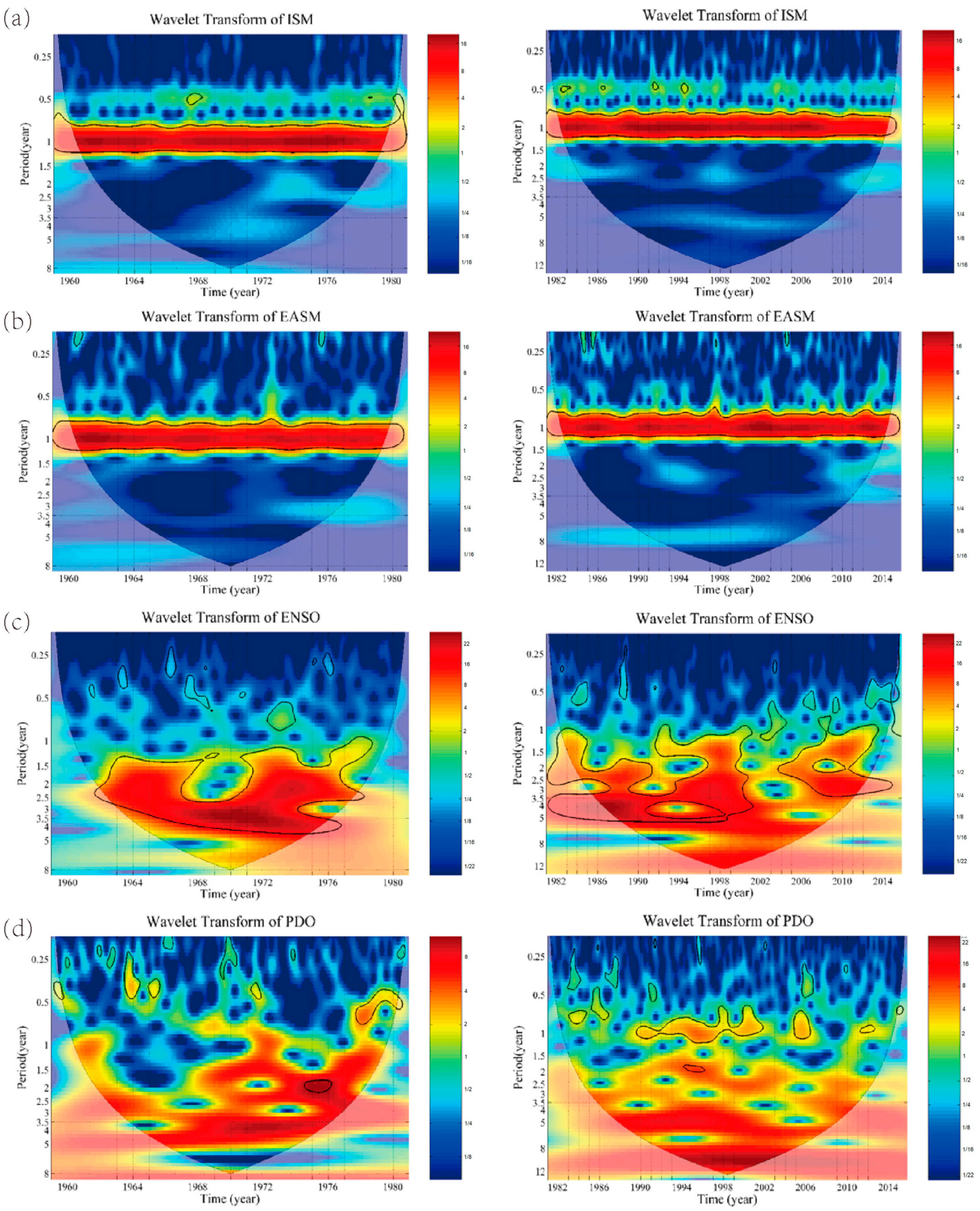
4.4. CWT of the Climate Phenomenon, Precipitation and the Spring Discharge

CWT technique was implemented to detect the primary modes of oscillation within time series of monthly climate influences, such as ISM, EASM, ENSO, PDO, precipitation, and spring discharge. It is worth mentioning that a significant level of 0.05 was used for periodicities greater than or equal to one year, while a more stringent significant level of 0.01 was applied to periodicities less than one year. The selection of the significant level was aimed at excluding white noise of high frequencies.

Figure 3a showed that ISM exhibited a continuous periodicity of 1 year during the pre- and post-development periods. Figure 3b illustrated that EASM mainly possessed continuous periodicity of 1 year during the both periods. Figure 3c showed that the periodicities of ENSO mainly concentrated at the time scales of 1 to 5 years in the pre- and post-development periods. Figure 3d illustrated the periodicities of PDO mainly focused on 0.5 years in pre-development period, and 0.5 to 1 year in the post-development period. Thus, for the monsoons, both ISM and EASM exhibited an obvious periodicity of 1 year, and for the climate teleconnections, ENSO has periodicities of 1 to 5 years, and PDO possesses periodicities of 0.5 to 1 year. Moreover, the ISM, EASM, and ENSO keep the same periodicities between the pre- and post-development periods, while PDO is a little different (

Table 2. The periodicity of indices in the pre-development and post-development period by wavelet analysis (year).

Indices	Pre-Development	Post-Development
ISM	1	1
EASM	1	1
ENSO	1–5	1–5
PDO	0.25–0.5	0.5 and 1
Precipitation	0.25–0.5 and 1	0.25–0.5 and 1
Spring discharge	0.25–1	0.25–1

). Because most of the climate indices keep the same periodicities, one can detect the spring discharge changes due to human activity by correlations of the climate indices with spring discharge between the two periods.

Figure 4a showed that precipitation exhibited a continuous periodicity of 1 year, and intermittent periodicities of 0.25–0.5 years in the pre- and post-development periods. Figure 4b illustrates that the spring discharge possessed fragmentary periodicities of 0.25–1 year during the middle and late 1960s and during the middle 1980s (Table 2). In karst hydrological processes, precipitation infiltrates to the subsurface, becoming groundwater, which flows through voids, fractures, and conduits, and then reaches outlets discharging as springs. In the process, the precipitation signals are attenuated due to resistance and storage of the karst aquifer. Only the strong precipitation signals can propagate through the karst aquifer and emerge as spring discharge. For this reason, the CWT coefficients of the spring discharge were weaker than those for precipitation. Even though the spring discharge signals were weak, the correlations of climate indices and precipitation with spring discharge were still significant. In other words, one can identify the spring discharge changes due to human activity by comparing the wavelet coherence coefficients of spring discharge with climate indices between pre- and post-development periods.

4.5. Wavelet Coherence of Precipitation and Spring Discharge with ISM

Figure 5a shows the continuous periodicity of 1 year and the intermittent periodicity of 0.5 and 2 years exhibited between precipitation and ISM in the pre-development period. The continuous periodicity of 1 year and intermittent periodicity of 0.5 and 2.5 years is exhibited between precipitation and ISM in the post-development period (Figure 5b). Moreover, the global coherence coefficients of precipitation with ISM at periodicities of 0.5 and 1 year were very close between the two periods, respectively (Figure 5e). However, the differences of the global coherence coefficients of precipitation with ISM were observed at inter-annual time scales between the two periods (Figure 5e). The results indicated that ISM affects precipitation stably at intra-annual and annual time scales, but impacts precipitation at inter-annual time scale unstably.

Similarly, the correlation between spring discharge and ISM is exhibited during the pre-development period in Figure 5c, particularly in terms of intermittent periodicity around 0.5 and 1 year. On the other hand, the intermittent periodicity around 0.5, 1, 2.5, and 5 years is exhibited in the post-development period (Figure 5d). Further, the global coherence coefficients of the spring discharge with ISM around periodicities of 0.5 and 1 year were observed in both pre- and post-development periods, which means that human activity could not alter the resonant periodicities of the spring discharge with ISM at intra-annual and annual time scales (Figure 5f). However, the inconsistencies of global coherence coefficients of the spring discharge with ISM at inter-annual time scales were observed between the two periods. This finding indicates that human activity caused a variation in the resonance patterns of the spring discharge with the ISM. In addition, the global coherence coefficients of precipitation with ISM were much larger than that of the spring discharge with ISM (Figure 5f). The results suggest that when precipitation infiltrated into the subsurface and propagated through the aquifer, its signals were attenuated.

4.6. Wavelet Coherence of Precipitation and Spring Discharge with EASM

Figure 6a displays the continuous periodicity of 1 year and the intermittent periodicity of 0.5 and 8 years exhibited between precipitation and EASM in the pre-development period. The continuous periodicity of 1 year and the intermittent periodicity of 0.5, 2, 3, and 8 years is exhibited between precipitation and EASM in the period after development (Figure 6b). Moreover, the coherence coefficients at 0.5- and 1-year periodicities between EASM and global precipitation were highly similar in both periods (Figure 6e). Meanwhile, during the two observed periods, variations in global coherence coefficients of precipitation and EASM were noted at inter-annual time scales. The observations implied that the impact of EASM on precipitation was consistent on an annual and intra-annual basis; its impact becomes unpredictable at an inter-annual time scale.

Similarly, Figure 6c illustrates the intermittent periodicity around 0.4 and 1 year exhibited between spring discharge and EASM during the pre-development period. On the other hand, the intermittent periodicity around 0.4, 1, 2.4, and 7 years is exhibited between spring discharge and EASM in the post-development period (Figure 6d). The coherence coefficients for the spring discharge with EASM showed consistent global values in the two periods, specifically around the 0.4-year and 1-year periodicities, which suggested that human activity could not alter the resonant periodicities of the spring discharge with EASM at intra-annual and annual time scales (Figure 6f). However, the inconsistencies of the global coherence coefficients of the spring discharge with EASM were observed at inter-annual periodicities between two periods, which revealed that the resonant periodicities of the spring discharge with EASM were altered by human activity.

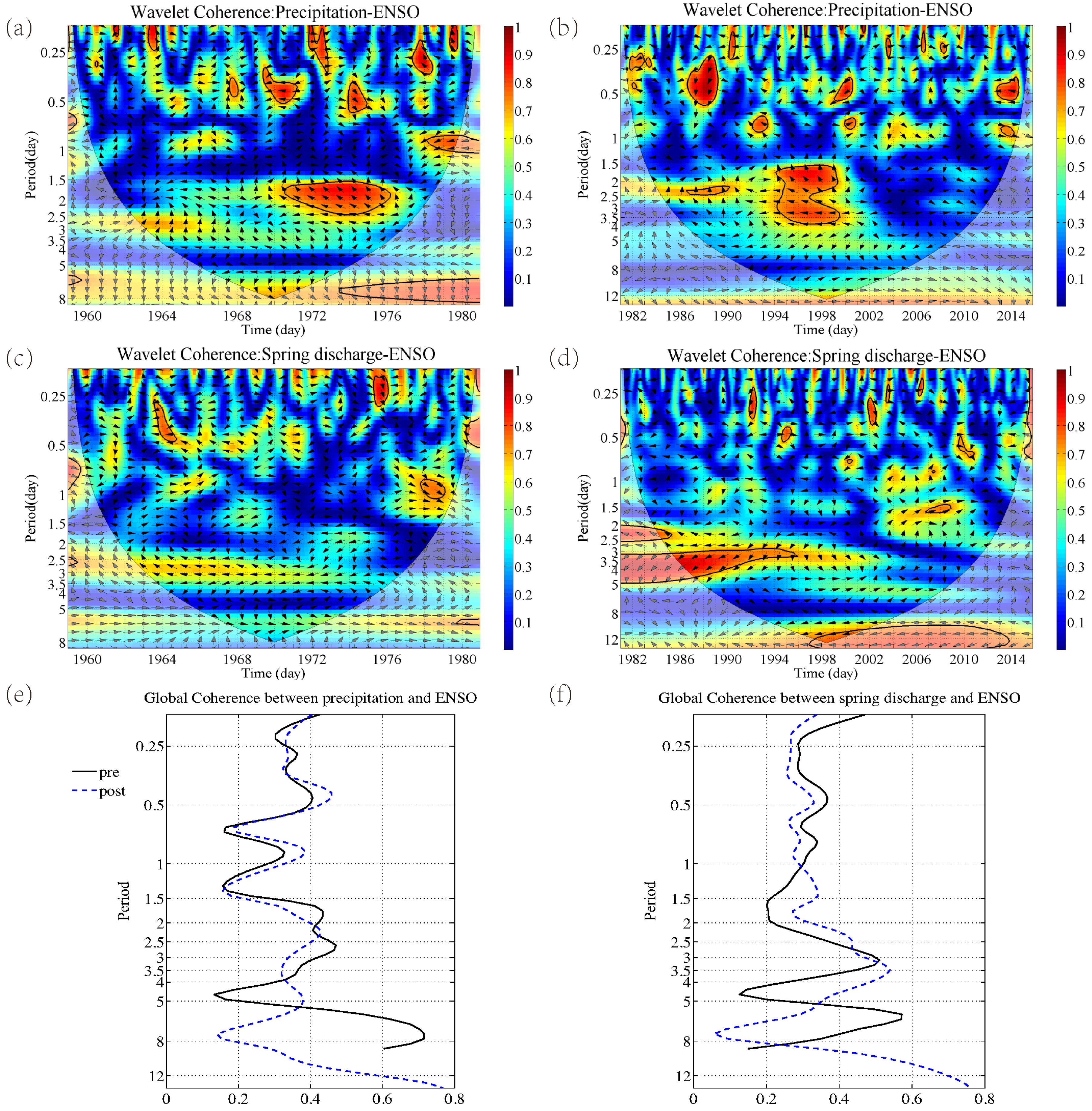
4.7. Wavelet Coherence of Precipitation and Spring Discharge with ENSO

Figure 7a shows the intermittent periodicities around 0.4, 0.8, and 2 years exhibited between precipitation and ENSO in the pre-development period. The intermittent periodicity around 0.4, 0.8, and 3 years is exhibited between precipitation and ENSO in the post-development period (Figure 7b). Moreover, the global coherence coefficients of precipitation with ENSO around periodicities of 0.4, 0.8, and 2–3 years were close between the two periods, respectively (Figure 7e). The results indicated that ENSO mainly affected precipitation in the NS basin at intra-annual and inter-annual time scales.

Similarly, Figure 7c,d illustrates the intermittent periodicities around 0.4, 0.8, and 3 years exhibited between the spring discharge and ENSO in the two periods. Moreover, the global coherence coefficients around periodicities of 0.4, 0.8, and 3 years were observed in the two periods, respectively (Figure 7f). Through comparing the global coherence coefficients of the spring discharge with ENSO between pre- and post-development, one can conclude that the human activity did not alter the resonant periodicities of ENSO with the spring discharge.

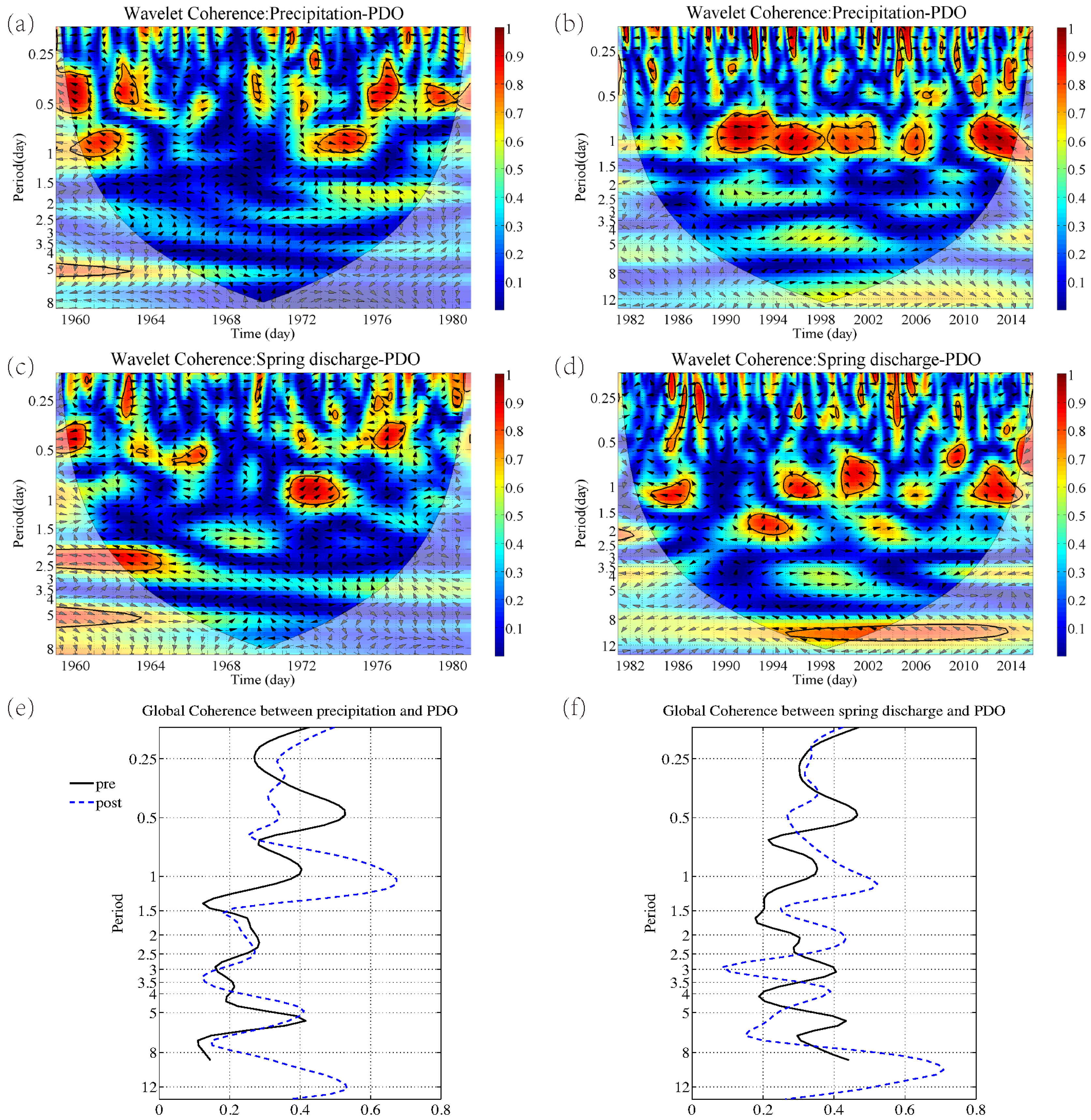
4.8. Wavelet Coherence of Precipitation and Spring Discharge with PDO

Figure 8a,b shows the intermittent periodicities around 0.5 and 1 year exhibited between precipitation and PDO in the two periods. Although the periodicity of 5 years was still observed between the two periods, it was out of the COI in pre-development, and did not pass the test of 0.05 significance level in post-development. Thus, the resonant periodicity of 5 years was negligible. Figure 8e illustrated that the global coherence coefficients of precipitation with PDO around periodicities of 0.5 and 1 year were consistent between the two periods. However, the coefficient values were small with large differences, which indicated that the effects of PDO on precipitation were weak in the NS basin.

As shown in Figure 8c, in the pre-development period, there were intermittent periodicities at 0.5-, 1-, and 2.5-year intervals in the correlations between spring discharge and PDO. However, in the post-development period, there were intermittent periodicities at 1- and 2-year intervals in the correlations between spring discharge and PDO (Figure 8d). Figure 8f illustrates that the global coherence coefficients of the spring discharge with PDO around periodicities of 1, and 2 years were consistent between the two periods. However, the coefficient values were small with large differences, which demonstrated that the effects of PDO on the spring discharge were weak.

By comparing the global coherence coefficients of both monsoons (ISM and EASM) and climate teleconnections (ENSO and PDO) with precipitation, one can find that the former was much larger than latter. The results emphasized that the monsoons were dominate climate factors that affected precipitation in the NS basin. In a similar way, the monsoons also were dominate climate factors that affected the spring discharge.

4.9. NSGEV for the Spring Discharge Minima

To investigate the spring discharge minima distribution during the pre-development and post-development periods, NSGEV models were set up for such two periods, respectively. The parameters of NSGEV distribution were identified by the maximum likelihood. NSGEV distribution for the pre-development period was

$$\tilde{G}\left(Q_1\right)=1-\exp \{-[1-0.525(\frac{Q_1-11.751}{1.460}){]}^{1/0.525}\}$$

(9)

where $Q_1$ represents the spring discharge minima during the pre-development period; $\tilde{G}\left(Q_1\right)$ represents the spring discharge minima distribution during the pre-development period.

The NSGEV model for the post-development period was set up by using the spring discharge minima from 1981 to 2012. The remaining spring discharge minimum values from 2013 to 2015 were used to validated the model (

Table 3. The prediction of the spring discharge minima (m³/s).

Year	Observed Spring Discharge Minima	Predicted Values	95% Confidential Intervals
			Upper Boundary	Lower Boundary
2013	5.96	5.20	6.73	3.47
2014	6.29	5.10	6.64	3.37
2015	5.81	5.00	6.54	3.27
2016		4.91	6.45	3.18
2017		4.82	6.35	3.09
2018		4.72	6.26	2.99
2019		4.62	6.16	2.90
2020		4.53	6.07	2.80

).

$$\tilde{G}(Q_2)=1-\exp \{-[1-0.212(\frac{Q_2-8.662+0.095t}{0.805}){]}^{1/0.212}\}$$

(10)

where $Q_2$ represents the spring discharge minima during the pre-development period; $\tilde{G}\left(Q_2\right)$ represents the spring discharge minima distribution during the post-development period.

Equation (9) showed that local parameter ${\mu }_t$ (i.e., 11.751), scale parameter ${\sigma }_t$ (i.e., 1.460), and shape parameter ${\xi }_t$ (i.e., −0.525) were constant during the pre-development period. In other words, the spring discharge minima were stationary under natural conditions. Equation (10) showed that local parameter ${\mu }_t$ (i.e., 8.662 − 0.095t) varied with time, and that scale parameter ${\sigma }_t$ (i.e., 0.805) and shape parameter ${\xi }_t$ (i.e., −0.212) were constant during the post-development period. The downtrend of the local parameter indicated that human activity caused the spring discharge minima to decline.

Using Equation (10), we predicted the spring discharge minima from 2013 to 2020 (Table 3). Table 3 shows that the spring discharge minima (i.e., from 2013 to 2015) used for model validation would fall in the 95% confidential interval. Thus, the model was accurate, and the results were confidential. Results also showed that on average, the spring discharge minima was supposed to be 4.53 m³/s in 2020, and its upper boundary of 95% confidence was supposed to be 6.07 m³/s, and its lower boundary of 95% confidence was supposed to be 2.80 m³/s.

5. Conclusions

Since the 1980s, the rapid development and exploitation of karst water resources in the Niangziguan basin have led to a decline in spring discharge. In order to better analyze the impact of human activities and climate variation on spring discharge, this study distinguished the monthly spring discharge data from January 1959 to December 2015 through cluster analysis. From the investigation, we conclude that the climate variation accounted for 6.93% of the NS discharge decline, while human activity caused 32.38% of the NS discharge decline on average since 1981.

Compared with the results of the wavelet analysis during the two periods, it can be seen that the monsoons (ISM and EASM) were dominate climate factors that affected the NS discharge versus climate teleconnections (ENSO and PDO). Most of the climate indices (i.e., ISM, EASM, and ENSO) keep the same periodicities. A comparison of wavelet coherence coefficients of spring discharge with climate indices during pre- and post-development periods can help to identify the impact of human activity on spring discharge. Human activity affected the periodicity of NS discharge depending on the time scales. That is to say, human activity could alter the resonant periodicities of the spring discharge with climate indices at inter-annual time scales, but the resonant periodicities at intra-annual and annual time scale remained the same between the two periods.

Human activity caused the fact that the local parameter of (non-stationary general extreme value) NSGEV distribution varied with time in a downward trend. The spring discharge minima was supposed to be 4.53 m³/s with a 95% confidential interval with an upper boundary of 6.06 m³/s and a lower boundary of 2.80 m³/s in 2020.

A karst spring is the natural discharge point of an aquifer, and its discharge variation reflects the regional change of groundwater level. In general, the methods developed in this study can be applied to many other karst springs in northern China. This study has taken a solid step towards utilizing meteorological changes to predict groundwater resources variation. However, a karst aquifer is generally highly uneven. The impact of climate change and human activities on spring discharge often lags behind, and we will explore this topic in more depth in the future.

References

1. Panno, S.V.; Kelly, W.R.; Scott, J.; Zheng, W.; McNeish, R.E.; Holm, N.; Hoellein, T.J.; Baranski, E.L. Microplastic Contamination in Karst Groundwater Systems. Ground Water 2019, 57, 189–196. [Google Scholar] [CrossRef]
2. Kovačič, G.; Petrič, M.; Ravbar, N. Evaluation and Quantification of the Effects of Climate and Vegetation Cover Change on Karst Water Sources: Case Studies of Two Springs in South-Western Slovenia. Water 2020, 12, 3087. [Google Scholar] [CrossRef]
3. Zhang, L.; Qin, X.; Tang, J.; Liu, W.; Yang, H. Review of arsenic geochemical characteristics and its significance on arsenic pollution studies in karst groundwater, Southwest China. Appl. Geochem. 2017, 77, 80–88. [Google Scholar] [CrossRef]
4. Xu, Z.; Hu, B.X.; Xu, Z.; Wu, X. Numerical study of groundwater flow cycling controlled by seawater/freshwater interaction in Woodville Karst Plain. J. Hydrol. 2019, 579, 124171. [Google Scholar] [CrossRef]
5. Jimenez-Martinez, J.; Smith, M.; Pope, D. Prediction of groundwater-induced flooding in a chalk aquifer for future climate change scenarios. Hydrol. Process. 2016, 30, 573–587. [Google Scholar] [CrossRef]
6. Charlier, J.; Ladouche, B.; Maréchal, J. Identifying the impact of climate and anthropic pressures on karst aquifers using wavelet analysis. J. Hydrol. 2015, 523, 610–623. [Google Scholar] [CrossRef]
7. Fiorillo, F.; Petitta, M.; Preziosi, E.; Rusi, S.; Esposito, L.; Tallini, M. Long-term trend and fluctuations of karst spring discharge in a Mediterranean area (central-southern Italy). Environ. Earth Sci. 2015, 74, 153–172. [Google Scholar] [CrossRef]
8. Schiperski, F.; Zirlewagen, J.; Hillebrand, O.; Nödler, K.; Licha, T.; Scheytt, T. Relationship between organic micropollutants and hydro-sedimentary processes at a karst spring in south-west Germany. Sci. Total Environ. 2015, 532, 360–367. [Google Scholar] [CrossRef]
9. Huo, X.; Liu, Z.; Duan, Q.; Hao, P.; Zhang, Y.; Hao, Y.; Zhan, H. Linkages between Large-Scale Climate Patterns and Karst Spring Discharge in Northern China. J. Hydrometeorol. 2015, 17, 713–724. [Google Scholar] [CrossRef]
10. Yuan, D. Karstology of China; Geological Publishing House: Beijing, China, 1994. (In Chinese) [Google Scholar]
11. Suksi, J.; Tullborg, E.-L.; Pidchenko, I.; Krall, L.; Sandström, B.; Kaksonen, K.; Vitova, T.; Kvashnina, K.O.; Göttlicher, J. Uranium remobilisation in anoxic deep rock-groundwater system in response to late Quaternary climate changes—Results from Forsmark, Sweden. Chem. Geol. 2021, 584, 120551. [Google Scholar] [CrossRef]
12. Rezaei, A.; Gurdak, J.J. Large-scale climate variability controls on climate, vegetation coverage, lake and groundwater storage in the Lake Urmia watershed using SSA and wavelet analysis. Sci. Total Environ. 2020, 724, 138273. [Google Scholar] [CrossRef] [PubMed]
13. Gumuła-Kawęcka, A.; Jaworska-Szulc, B.; Szymkiewicz, A.; Gorczewska-Langner, W.; Angulo-Jaramillo, R.; Šimůnek, J. Impact of climate change on groundwater recharge in shallow young glacial aquifers in northern Poland. Sci. Total Environ. 2023, 877, 162904. [Google Scholar] [CrossRef]
14. Tremblay, L.; Larocque, M.; Anctil, F.; Rivard, C. Teleconnections and interannual variability in Canadian groundwater levels. J. Hydrol. 2011, 410, 178–188. [Google Scholar] [CrossRef]
15. Saber, A.; Cheng, V.Y.S.; Arhonditsis, G.B. Evidence for increasing influence of atmospheric teleconnections on water levels in the Great Lakes. J. Hydrol. 2023, 616, 128655. [Google Scholar] [CrossRef]
16. Zhang, J.; Hao, Y.; Hu, B.X.; Huo, X.; Hao, P.; Liu, Z. The effects of monsoons and climate teleconnections on the Niangziguan Karst Spring discharge in North China. Clim. Dyn. 2017, 48, 53–70. [Google Scholar] [CrossRef]
17. Hao, Y.H.; Zhang, J.; Wang, J.J.; Li, R.F.; Hao, P.M.; Zhan, H.B. How does the anthropogenic activity affect the spring discharge? J. Hydrol. 2016, 540, 1053–1065. [Google Scholar] [CrossRef]
18. Song, X.; Hao, H.; Liu, W.; Wang, Q.; An, L.; Jim Yeh, T.-C.; Hao, Y. Spatial-temporal behavior of precipitation driven karst spring discharge in a mountain terrain. J. Hydrol. 2022, 612, 128116. [Google Scholar] [CrossRef]
19. Liang, Y.; Wang, W.; Zhao, C.; Wang, W.; Tang, C. Karst water variation characteristics and environmental problems in northern China. Ankengsin Karst China 2013, 32, 34–42. (In Chinese) [Google Scholar]
20. Shekhar, M.; Sharma, A.; Dimri, A.P.; Tandon, S.K. Asian summer monsoon variability, global teleconnections, and dynamics during the last 1000 years. Earth-Sci. Rev. 2022, 230, 104041. [Google Scholar] [CrossRef]
21. Liu, Y.; Liang, P.; Sun, Y. Chapter 8—Northern Teleconnection between the Indian Summer Monsoon and Rainfall Anomalies in Northern China. In The Asian Summer Monsoon; Elsevier: Amsterdam, The Netherlands, 2019; pp. 135–155. [Google Scholar]
22. Hau, N.-X.; Sano, M.; Nakatsuka, T.; Chen, S.-H.; Chen, I.C. The modulation of Pacific Decadal Oscillation on ENSO-East Asian summer monsoon relationship over the past half-millennium. Sci. Total Environ. 2023, 857, 159437. [Google Scholar] [CrossRef]
23. Fu, S.; Zhang, H.; Zhong, Q.; Chen, Q.; Liu, A.; Yang, J.; Pang, J. Spatiotemporal variations of precipitation concentration influenced by large-scale climatic factors and potential links to flood-drought events across China 1958–2019. Atmos. Res. 2023, 282, 106507. [Google Scholar] [CrossRef]
24. Niu, T.; Wang, J.; Yang, Y.; Jiang, X.; Jiang, Y.; Che, H. The impact of the large-scale circulation anomalies in the northern hemisphere on air quality in Wuhan of China during the Spring Festival in 2020. J. Atmos. Sol. Terr. Phys. 2022, 238–239, 105931. [Google Scholar]
25. An, L.; Hao, Y.; Yeh, T.-C.J.; Liu, Y.; Liu, W.; Zhang, B. Simulation of karst spring discharge using a combination of time–frequency analysis methods and long short-term memory neural networks. J. Hydrol. 2020, 589, 125320. [Google Scholar] [CrossRef]
26. Han, X.; Lu, R.; Li, Q. Karst Water Systems: A Study on Big Karst Spring in Shanxi; Geological Publishing House: Beijing, China, 1993. (In Chinese) [Google Scholar]
27. Hu, C.; Hao, Y.; Yeh, T.C.J.; Pang, B.; Wu, Z. Simulation of spring flows from a karst aquifer with an artificial neural network. Hydrol. Process. 2008, 22, 596–604. [Google Scholar] [CrossRef]
28. Liang, Y.; Gao, H.; Zhang, J.; Huo, J.; Wang, T. Preliminary quantitative analysis on the causes of discharge attenuation in Niangziguan spring. Carsologica Sin. 2005, 24, 227–231. (In Chinese) [Google Scholar]
29. Yuan, R.; Li, Z.; Guo, S. Health risks of shallow groundwater in the five basins of Shanxi, China: Geographical, geological and human activity roles. Environ. Pollut. 2023, 316, 120524. [Google Scholar] [CrossRef]
30. Fan, Y.; Huo, X.; Hao, Y.; Liu, Y.; Wang, T.; Liu, Y.; Yeh, T.J. An assembled extreme value statistical model of karst spring discharge. J. Hydrol. 2013, 504, 57–68. [Google Scholar] [CrossRef]
31. Zhang, H.; Guo, Y.; Miu, P.; Sun, K. Analysis on the status of water ecological investigation in Niangziguan spring area and the cause of spring discharge attenuation. China Environ. Sci. Soc. Acad. Essays 2014. (In Chinese) [Google Scholar]
32. Fotsing, C.; Menadjou, N.; Bobda, C. Iterative closest point for accurate plane detection in unorganized point clouds. Autom. Constr. 2021, 125, 103610. [Google Scholar] [CrossRef]
33. Takio, K. Principal component analysis (PCA). In Computer Vision; Katsushi, I., Ed.; Springer: New York, NY, USA, 2014; pp. 636–639. [Google Scholar]
34. Yeh, Y.-C.; Wu, H.-A.; Huang, F. Exploring profiles of varied types of achievement goals, emotions and digital insight problem solving through cluster analysis. Think. Skills Creat. 2022, 46, 101170. [Google Scholar] [CrossRef]
35. Asmita, R.M.; Dhyan, S.A. Trend and periodicity analysis in rainfall pattern of Nira Basin, Central India. Am. J. Clim. 2014, 3, 60–70. [Google Scholar]
36. Zhang, Y.; Wang, M.; Zipperle, M.; Abbasi, A.; Tani, M. RelRank: A relevance-based author ranking algorithm for individual publication venues. Inf. Process. Manag. 2023, 60, 103156. [Google Scholar] [CrossRef]
37. Dao, P.B. On Wilcoxon rank sum test for condition monitoring and fault detection of wind turbines. Appl. Energy 2022, 318, 119209. [Google Scholar] [CrossRef]
38. Yan, Y.; Li, J.; Huai, N.; Guan, J.; Liu, H. Two-station analysis of passive surface waves with continuous wavelet transform and plane-wave-based beamforming. J. Appl. Geophys. 2022, 197, 104526. [Google Scholar] [CrossRef]
39. Kriechbaumer, T.; Angus, A.; Parsons, D.; Casado, M.R. An improved wavelet-ARIMA approach for forecasting metal prices. Resour. Policy 2014, 39, 32–41. [Google Scholar] [CrossRef]
40. Torrence, C.; Compo, G.P. A practical guide to wavelet analysis. Bullet. Am. Meteorol. Soc. 1998, 79, 61–78. [Google Scholar] [CrossRef]
41. Abebe, S.A.; Qin, T.; Zhang, X.; Yan, D. Wavelet transform-based trend analysis of streamflow and precipitation in Upper Blue Nile River basin. J. Hydrol. Reg. Stud. 2022, 44, 101251. [Google Scholar] [CrossRef]
42. Pagliaroli, T.; Gambioli, F.; Saltari, F.; Cooper, J. Proper orthogonal decomposition, dynamic mode decomposition, wavelet and cross wavelet analysis of a sloshing flow. J. Fluids Struct. 2022, 112, 103603. [Google Scholar] [CrossRef]
43. Liu, Y.; Hao, Y.; Fan, Y.; Wang, T.; Huo, X.; Liu, Y.; Yeh, T.J. A nonstationary extreme value distribution for analyzing the cessation of karst spring discharge. Hydrol. Process. 2014, 28, 5251–5258. [Google Scholar] [CrossRef]
44. Coles, S. An Introduction to Statistical Modeling of Extreme Values; Springer: New York, NY, USA, 2001. [Google Scholar]
45. Magee, L. Nonlocal behavior in polynomial regressions. The American Statistician. Am. Stat. Assoc. 1998, 52, 20–22. [Google Scholar]
Figure 1. Schematic diagram of the NS basin and its geographic location.
Sustainability 15 08798 g001
Figure 2. Monthly spring discharge and precipitation from 1959 through 2015 in Niangziguan Springs Basin.
Sustainability 15 08798 g002
Figure 3. Wavelet analysis for ISM (a), EASM (b), ENSO (c), and PDO (d) in pre-development (left) and post-development (right) stages.
Sustainability 15 08798 g003
Figure 4. Wavelet analysis for precipitation (a) and spring discharge (b) in pre-development (left) and post-development (right) stages.
Sustainability 15 08798 g004
Figure 5. Wavelet coherence of precipitation (a,b), and the spring discharge (c,d) with ISM in the pre- and post-development stages. Global coherence coefficients of precipitation (e) and the spring discharge (f) with ISM in the pre- and post-development stages.
Sustainability 15 08798 g005
Figure 6. Wavelet coherence of precipitation (a,b), and the spring discharge (c,d) with EASM in the pre- and post-development stages. Global coherence coefficients of precipitation (e) and the spring discharge (f) with EASM in the pre- and post-development stages.
Sustainability 15 08798 g006
Figure 7. Wavelet coherence of precipitation (a,b) and the spring discharge (c,d) with ENSO in the pre- and post-development stages. The global coherence coefficients of precipitation (e) and the spring discharge (f) with EASM in the pre- and post-development stages.
Sustainability 15 08798 g007
Figure 8. Wavelet coherence of precipitation (a,b) and the spring discharge (c,d) with PDO in the pre- and post-development periods. Global coherence coefficients of precipitation (e) and the spring discharge (f) with PDO in the pre- and post-development periods.
Sustainability 15 08798 g008