A Bridge Damage Visualization Technique Based on Image Processing Technology and the IFC Standard

Abstract

As an important part of the traffic infrastructure, the bridge has attracted much attention for its health conditions. Bridge damage detection is an important way of evaluating bridge health conditions. However, the bridge damage could not be directly expressed by traditional bridge damage detection methods. With the emergence of new technologies and engineering applications, it is possible to achieve visual expression of bridge damages, improve the digitization of bridge detection, and promote sustainable development in bridge maintenance. In this paper, a method of bridge damage visualization based on image processing technology and the IFC standard description is proposed for common bridge damages. An existing cable-stayed bridge is taken as the engineering background, and the collected damage images are processed and analyzed utilizing cutting-edge technology to obtain specific damage information such as the length and width of bridge cracks and concrete defects. Then based on the IFC standard, the bridge damage and its attribute information are visualized and stored through an established REVIT model of the bridge.

1. Introduction

At present, the bridge damage is mainly detected by the technicians using special equipment. Normally, to represent the bridge damage detection result, the obtained information from the detection equipment would be summarized into a report. The traditional method needs to consult a large number of documents to obtain specific information about bridge damage, which is time-consuming and inefficient. To improve the accuracy of the bridge damage identification, the damage detection technology based on visualization technique is adopted in the engineering application. Meanwhile, in order to facilitate the bridge stakeholders to obtain the bridge damage information directly, the damage information can be displayed in the three-dimensional digital model of the bridge to improve the digitalization degree of the bridge operation and maintenance.

Digital image processing emerged in the 1920s, and in the early days of transportation, it was primarily used for crack detection on asphalt road surfaces. This is because asphalt road surfaces lend themselves to clear image acquisition. As image acquisition technology continued to improve, digital image processing gradually found application in the detection of damage on bridges. Firstly, methods regarding image processing are examined. Jin et al. [1,2,3] successfully eliminated edge burrs in the binary image of cracks by using erosion and dilation operations with different coefficients, thereby improving the quality of image processing. Wang [4] proposed an image segmentation algorithm based on the SSA (Singular Spectrum Analysis) method, which was used to segment image thresholds, and compared five threshold segmentation methods. The results showed that Otsu (Otsu’s method), PSO (Particle Swarm Optimization), and SSA had similar thresholds and good segmentation effects. This method can make image processing more effective. Zuo et al. [2] combined iterative method with threshold method for image processing, using histogram peak-valley method for image segmentation, and compared the effects of Kittler binarization and Niblack binarization. The conclusion was that Kittler binarization was more effective, which was of great help for image binarization processing. Xiao et al. [5] proposed an improved median filtering algorithm based on differential threshold judgment, and used Otsu threshold segmentation method to extract cracks. Cevallos-Torres L J et al. [6] compared different segmentation techniques and concluded that the Canny edge detection method provided the best evaluation technique. Secondly, the method of collecting information about the image was studied. Jin et al. [1] used the minimum bounding rectangle method to detect the size of crack images. Tan et al. [7] obtained the pixel length of cracks by calculating the Euclidean distance between each adjacent center point, and pasted a solid color block on the surface of the concrete structure as a calibration block, which was converted to obtain the actual length of cracks. Wang et al. [3] obtained the total number of pixels on the length and width of cracks through the step-line approximation. Shao et al. [8] used the region connecting method to connect regions filled with multiple seed points to extract complete bridge cracks. Shi et al. [4,9] used the boundary extraction method based on chain code to obtain information such as the length, width, and area of cracks. Shen et al. [2,5,6,10] used the skeleton method to determine the length and average width of cracks. The research results of the above researchers provide an important theoretical and practical basis for future research on image processing.

Then, in order to realize the visual expression of bridge cracks and defects in BIM model, IFC data format is generally used to describe the information. The IFC standard has been gradually improved, which can store specific information of model entities and display it on BIM-related software, providing the possibility for the realization of visual expression of bridge damage based on IFC [11,12,13,14]. Xu et al. [12] described the relationship between defects and other IFC entities through parametric modeling of the geometric structure of defects. Chu et al. [15,16,17,18] studied the specific compilation process of component geometric models realized by IFC statements, proposed a parametric modeling method of model damage based on the IFC standards, and visualized concrete cracks. Philipp Hüthwohl et al. [19] verified that the latest version of IFC can serve as the basis for integrating relevant defect information and images. Dušan Isailović et al. [20] integrated the damaged component into the BIM by enriching the semantics of the IFC model.

This paper realizes the visualization of bridge damages by using MATLAB and REVIT software. Firstly, the image is processed by multiple tools to get the damage information. The image is grayed by the weighted average method, and the gray adjustment enhances the image. The linear filter and the Otsu binarization method are used to denoise and segment the image. The final binary image is obtained by removing the interference of small area images and morphological calculation. Secondly, the length of the processed crack image was calculated by the skeleton method, and the width and area were calculated by the pixel point statistics method. Finally, the damage model is established by using the boundary representation method. Through points, lines, surfaces and their mutual relations, an object is represented as many curved surfaces connected to form a closed space area to form a bridge model with damage.

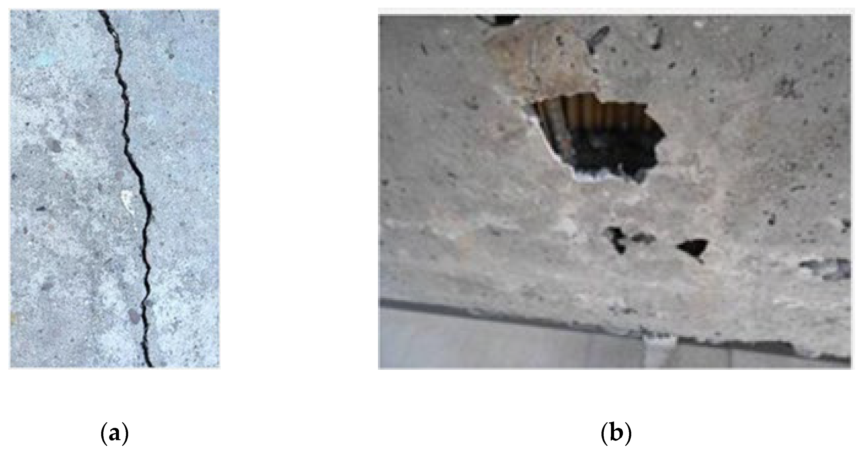
2. Damage Information Collection Based on Image Processing Technology

2.1. Image Processing

Due to practical reasons, the process of damage image acquisition will be affected by many factors, and the collected images are often complex in illumination and excessive in noise. In order to obtain more intuitive images and facilitate the collection of image information in the later work, the images need to be processed by MATLAB. The original images of the damages are shown in Figure 1.

• Graying

Generally, the acquired damaged images are color images, that is, the R, G, and B components determine the color of each pixel. For 8-bit images, the value range of each component is [0, 255], and the number of colors is 16,777,216. The information content is too large, so it is inconvenient to process. To simplify the image matrix, enhance the clarity of image information, and facilitate the extraction of later image information, grayscale processing can be applied to the image as a preliminary step. After gray scale processing, each pixel of the image has only one sampling color, that is, the number of colors is reduced to 256, and the redundant information can be simplified [9]. Weighted average method can be used to transform image gray scale [5].

2.

Image enhancement

Affected by material and environmental factors, the collected damage images will likely have problems such as uneven light and dark, background clutter, and image distortion. In order to solve these problems and better contrast and separate the foreground and background, image enhancement is required. Spatial domain processing is a commonly used image processing method. The image enhancement method includes histogram equalization and gray adjustment. Comparing these two methods shows that histogram equalization can amplify the noise in the image when the original image contrast is not strong, and the contrast needs to be adjusted to enhance the limit. The gray adjustment method can better avoid such problems. Therefore, the gray adjustment method can map the input intensity image value to the new value to improve the contrast and enhance the image.

3.

Noise processing

Environment noise and other factors will negatively impact the damage image processing, resulting in the final image with unnecessary pixel points or pixel blocks formed by noise, resulting in errors in the subsequent information extraction. Therefore, it is necessary to remove the noise in the image. The adaptive filter function Wiener2 is used in MATLAB, which filters the image with pixel type adaptive filter and applies the Wiener filter (a linear filter) to the image in an adaptive way, which usually produces better results than the linear filter. The specific steps of the Wiener2 algorithm are outlined as follows: for each pixel of the input image, Wiener2 meticulously computes the local mean and variance of the neighboring pixels in the immediate vicinity. Subsequently, utilizing these local statistics, a pixel-level Wiener filter is skillfully constructed. Finally, Wiener2 employs this filter with adeptness to effectively eliminate the noise that is present in the image, thereby resulting in a more refined and visually clearer image.wiener2 estimates the local mean and variance around each pixel:

$$\mu =\frac{1}{NM}{\displaystyle \sum _{n1,n2\in \eta }a(n1,n2)}$$

(1)

$${\sigma }^2=\frac{1}{NM}{\displaystyle \sum _{n1,n2\in \eta }{a}^2(n1,n2)-{\mu }^2}$$

(2)

where, $\eta$ is the N × M local neighborhood of each pixel in the image. wiener2 uses these estimates to create a pixel-level Wiener filter:

$$b(n1,n2)=\mu +\frac{{\sigma }^2-{\nu }^2}{{\sigma }^2}(a(n1,n2)-\mu )$$

(3)

where, ${\nu }^2$ is the noise variance. If no noise variance is given, wiener2 uses the average of all local estimated variances [21].

4.

Image segmentation and post processing

Image segmentation is an important step before image analysis. The image segmentation is to separate the damage part from the background to avoid other factors in affecting the accuracy of information. The segmentation methods include threshold segmentation, region segmentation and edge segmentation. The binarization method is a kind of threshold segmentation widely used in image segmentation technology. It determines a threshold based on pixel intensity to convert the image into a binary graph with pixels represented by either 0 (black) or 1 (white). The deep crack pixel is usually processed as black when extracting crack information. However, since the value of a black pixel is zero, this processing method is inconvenient in calculating the number of pixel points in the crack image, so it is necessary to carry out the inverse operation on the image. In MATLAB, the inverse function can complement the binary image. The black and white are exchanged to achieve the effect that the crack damage is treated as white, and the background color is treated as black.

After image processing, it is necessary to extract the damaged information. In image processing, it is difficult to avoid empty pixel points. Therefore, before information extraction, it is necessary to fill the holes in binary pixels, delete the small area image and expand the image appropriately to avoid interference with subsequent information extraction. The damaged image after processing is shown in Figure 2.

2.2. Extracting Image Information

A black square block with an area of 1 cm² was selected as the image calibration block. During image collection, the calibration block and the damage image were placed in the same environment, and the same acquisition equipment was used to collect them. After that, the calibration block and the damage image were separated to extract the pixel number of the calibration block. According to the actual area and pixel number of the calibration block, the damage information was extracted and converted to obtain the actual damage information.

• Obtain crack length

The specific information on cracks is very important in assessing the bridge’s health condition, so after the completion of image processing, it is necessary to extract the damage information in the image. The crack length can be obtained by the skeleton method. In MATLAB, the bimorph function can extract the processed crack skeleton. However, the extracted crack has spikes, which must be eliminated after several operations. Finally, the crack skeleton formed by connecting single pixel points is obtained, as shown in Figure 3. The crack length can be obtained by calculating the number of pixels in the skeleton and converting them to the actual length in proportion.

2.

Obtain crack width

The width of each crack is obtained by adding up the elements of the post-processed binary image in the second dimension before skeletonizing and expanding the crack. Thus, the maximum width, minimum width, and average width of the crack can be approximately obtained. Calculating all pixel points in the binary image can also determine the crack area. The average crack width can be approximated by dividing the area by the length.

3.

The damage area is calculated by pixel points

In addition to cracks, other damages, such as concrete cavities and damage, are also common in bridge damage. In order to ensure the accuracy of image information of the defect area, it is unnecessary to conduct expansion processing and hole filling for the defect area image. The binary image generated after processing can directly count pixels. The real defect area can be obtained through pixel number and proportion conversion.

3. Expression of Bridge Damage Information

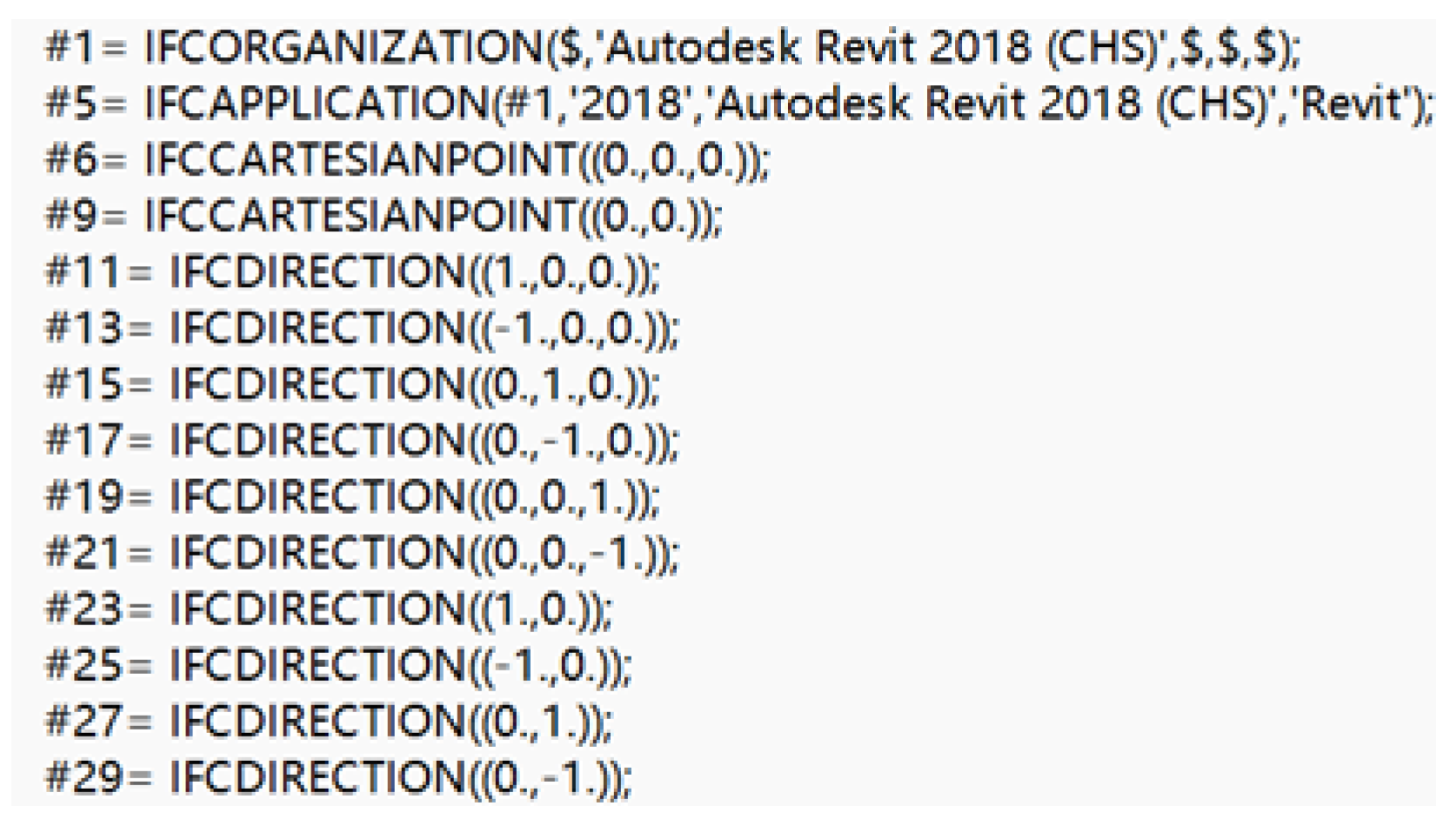
3.1. Characteristics of the IFC Architecture

IFC (Industry Foundation Classes) standard was developed by the American buildingSmart Organization (IAI), which is a standardized and digital description of the built environment (including buildings and civil infrastructure) [11]. IFC is described by EXPRESS language, which can better express data and has good readability. IFC’s data schema architecture defines four conceptual layers, the top layer is the domain layer, which provides specialized information for each domain, the bottom layer is the shared, core layer, which provides the shared, core layer of multiple domains, which contains the most common entity definition, and the resource layer, which defines the entity that describes the basic information of the model and cannot be used independently of the definition declared at the higher level [11,13,14,15,18].

IFC’s data structure is divided into header segment and data segment. The header section starts with header statement and ends with ENDSEC statement. The annotation symbols “/*” and “*/” include the annotation statement, which describes the creation date, IFC standard version, etc. The main statements in the header segment are file attribute (FILE_DESCRIPTION), file name (FILE_NAME) and file version (FILE_SCHEMA), which belong to file attribute type statements [15]. The DATA segment starts with the data statement and ends with the ENDSEC statement, which is the specific part of the file data description and belongs to the entity attribute type statement [15]. This type of statement begins with “#”, followed by the entity’s numeric ID, followed by the “=“ symbol is the entity type of IFC, parentheses are the attributes of the entity, separated by “, “, when referring to other entities, only need to be represented as “#” + numeric ID. “$” is commonly used to represent a placeholder for a null value or a value that is not provided. The specific description code is shown in Figure 4.

3.2. IFC Expression of Cracks

This modeling uses Revit2018 version, IFC standard uses 2 × 3 version, to establish concrete block and its crack model as an example to explain the basic theory of IFC expression.

The commonly used methods for the construction of geometric models through IFC files mainly include boundary representation, scanning representation (also known as stretching body representation), surface model method, structural solid geometry method and surface subdivision method. The basic process of concrete blocks created by scanning representation is to first draw a two-dimensional outline on the working plane, and then stretch the outline along a certain direction to form a three-dimensional object. The IFCEXTRUDEDAREASOLID statement can stretch a solid. This method is simple and intuitive in expression and suitable for graphic input. However, due to the difficulty in geometric transformation and the inability of this method to directly obtain the boundary information of the body, the coverage area of the representation is very limited. The boundary representation method represents an object as a closed space area formed by connecting many surfaces. It has more information about faces, edges, points and their relationships, and is suitable for damage modeling. The following describes the IFC file and the modeling process.

The IFC file first explains IFC related application information, and then defines Cartesian points and coordinate vectors. In Figure 4, #11~#21 are spatial coordinate vectors based on the three-dimensional plane, and #23~#29 are spatial coordinate vectors based on the two-dimensional plane. In addition, in the IFC file, there are also IFCSIUNIT statements that define various units, IFCAXIS2PLACEMENT3D statements that define the position and direction of objects in three-dimensional space, and IFCLOCALPLACEMENT statements that define the relative position of a product relative to another product or the absolute position of a product in the context of geometric representation of the project. The boundary notation requires the following commands: The IFCCARTESIANPOINT statement defines the vertex coordinates, the IFCPOLYLOOP statement connects the points to a line, the IFCFACEOUTERBOUND statement defines the surface boundary, the IFCFACE statement defines the ring-bounded surface of the shell, and finally the IFCCLOSEDSHELL Statement to implement the combination between the faces. The remaining commands are not relevant to this modeling, therefore, this article does not go into detail.

The cube is chosen as the concrete block model, and this concrete block model has 8 vertices. The coordinates of these 8 vertices are defined first, and then the cracks are modeled using a simple crack with 6 points on each of the inner and outer planes and a total of 8 faces as an example. The code related to the concrete block and crack modeling process is shown in Appendix A. The modeling process is shown in Figure 5.

The concrete block with cracks formed after completing the above steps is shown in Figure 6.

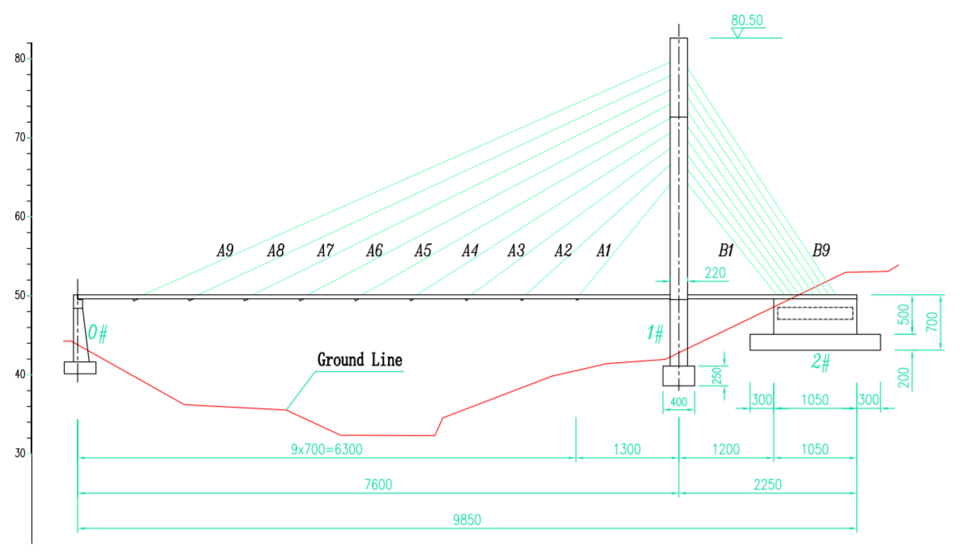
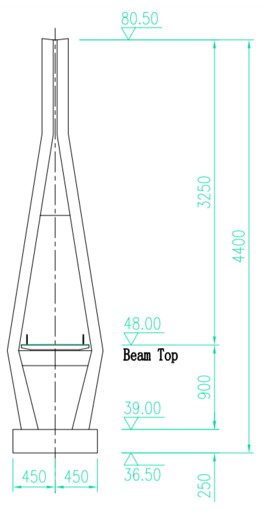
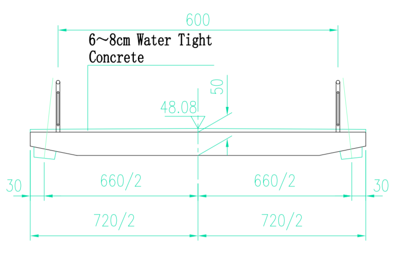
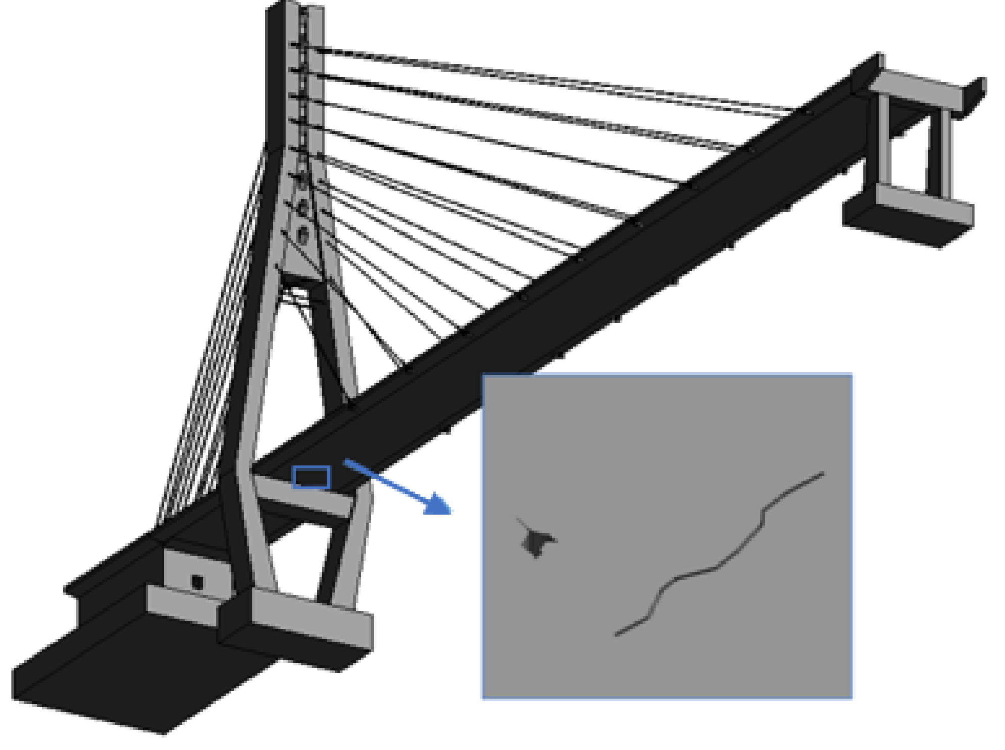
4. Visual Display of a Cable-Stayed Bridge Damage Information

4.1. Project Overview

The bridge is a single tower concrete cable-stayed bridge with a main span of 76 m and a total length of 98.5 m. The total width of the bridge is 7.2 m, and the width of the sidewalk is 6.0 m. The height of the main beam is 0.5 m. In the process of bridge use, it is difficult to avoid the phenomenon of concrete cracks, spalling, holes and reinforcement exposure, which will have adverse effects on the health of the bridge. In order to realize the image processing and visualization of bridge damage, this section takes the cable-stayed bridge as an example, and applies the image processing and visualization methods introduced above. The three-view drawings of the bridge are shown in Figure 7, Figure 8 and Figure 9.

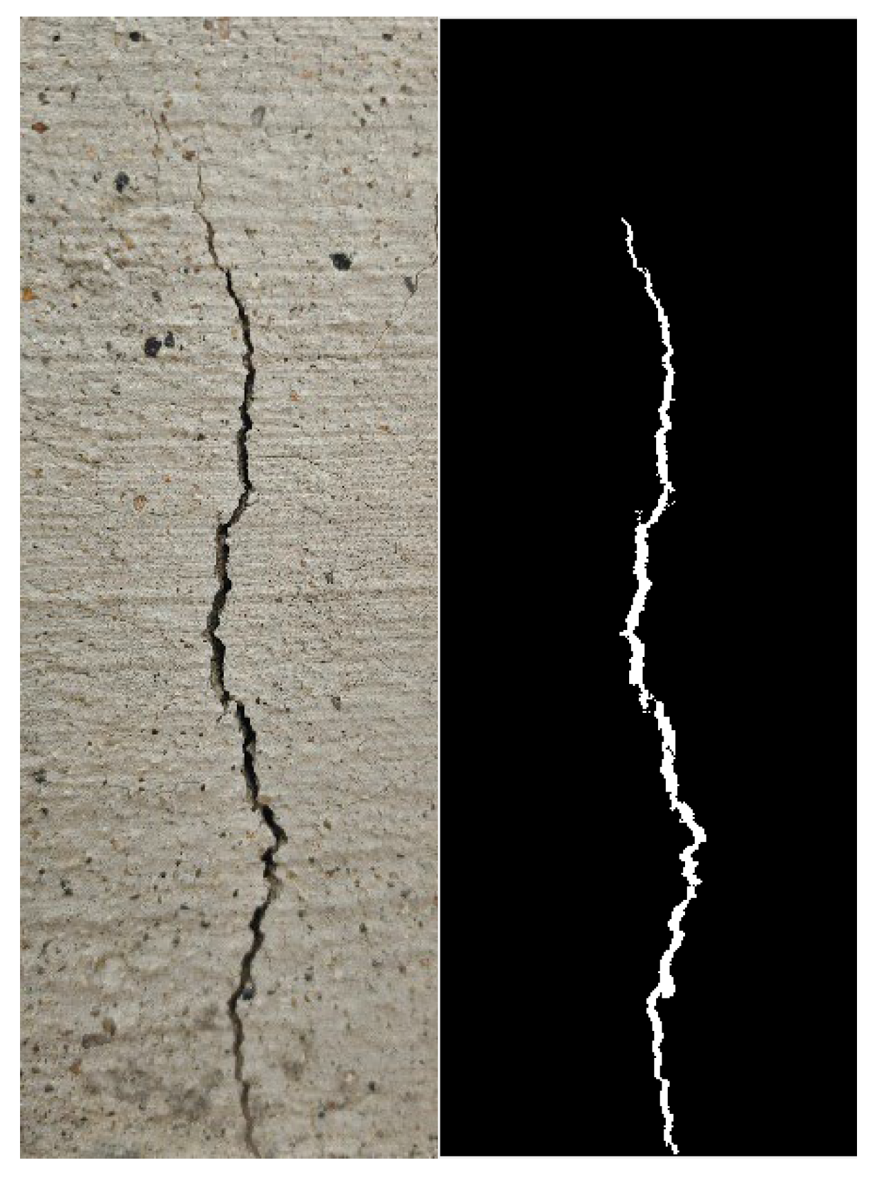
4.2. Collect and Process Damage Images

During bridge inspections, it is necessary to examine various types of damages that can occur in each part. Taking the upper structure of a cable-stayed bridge as an example, various components such as cables, cable towers, and main girders need to be inspected. Regarding the cables, inspections should cover whether there is cable corrosion, broken wires, coating damage, cracks, scratches, and paint damage, as well as the appearance of the PE (Polyethylene) sheath. For the cable towers, inspections should check for cracks, water seepage in the anchorage area, honeycomb, spalling, exposed reinforcement, and other phenomena. As for the main girders, inspections should cover whether there are cracks, water seepage, surface weathering, spalling, and exposed reinforcement in the interior and exterior concrete.

It can be seen from the above that there are many types of bridge damages. However, cracks, exposed reinforcement and other damages are the most common, and they have a noticeable impact on bridge health. Therefore, cracks and concrete defects are selected to realize damage visualization based on image processing and IFC standards.

The original crack drawing and the effect of drawing after treatment are shown in Figure 10. The crack length obtained through on-site measurement is 97 mm, and the width is 1.2 mm. Since there is only a single pixel point per row after the crack extraction skeleton, the image display may not be complete, and after zooming in, you can see the individual pixel points connected into a skeleton, as shown in Figure 11 and Figure 12. The total number of pixels in the entire image is 3540 × 1296 px. After the image processing, the total number of cracked pixel blocks is 87,480 through the command flow of the for a loop. Skeletonization transforms the shapes of objects in an image into their center-lines or skeletons. After skeletonization, the length pixel is 3109, and the width pixel is 37. According to the scale conversion between image pixels and actual size, it can be seen that the corresponding actual length of a pixel block is 0.0317 mm, so the actual length of the crack is 98.56mm, and the actual width of the crack is 1.17 mm. The difference between the calculated and actual sizes is less than 5%.

The original drawing of the concrete defect and the effect drawing after treatment are shown in Figure 13. The total number of pixels in the entire image is 912 × 860 px. After the image processing is completed, it can be obtained through the for loop command flow that the total number of pixel blocks in the concrete defect part is 79,245, Through the proportional conversion between the image and the actual size, it can be seen that the corresponding actual area of a pixel block is 0.0011 mm², and the calculated image area is 90.36 mm², namely 0.904 cm². The difference with the actual defect area S = 1 × 0.9 cm² is less than 1%, and the error is negligible.

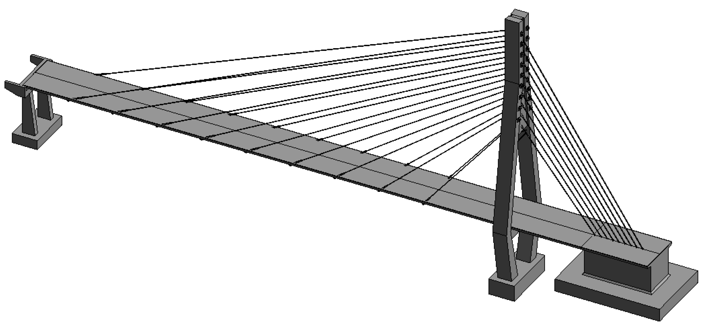
4.3. Establishment of Revit Model of Cable-Stayed Bridge

The process of creating a cable-stayed bridge using Revit 2018 is as follows:

• Create families for each component of the cable-stayed bridge.

Take the main beam as an example. In Revit, first create a new family, select “Metric Generic Model,” then change the family category to “Structural Framing” and set the family parameters. After that, modify the project units and set the dimension annotation according to the drawings, combine with the software’s stretching, merging, hollow shape and other tools to create a 3D solid model of the main beam. It should be noted that when using hollow stretching, the “Cancel Cut Geometry” command must be used to cancel the clipping of the main beam parts except for the anchorage area. After the creation is complete, save the family file. The completed main beam model is shown in Figure 14.

After the main beam is created, according to the design requirements of the cable-stayed bridge, refer to the steps of creating the main beam parameter family, and create parameter families for each component such as the bridge deck, bridge tower, pier, cable, and anchorage.

2.

Add family instances

After the cable-stayed bridge families are created, open the corresponding project file in Revit and select the family type to be added, and drag it into the project view.

3.

Adjust the position of the family

In the project view, by selecting the family instance of each component, use the move command to adjust the position of the pier, cable tower, main beam, and other family instances according to the drawing requirements.

4.

Add cables

In the project view, select the cable instance and use the “create instance” command to place it in the space between the bridge deck and the bridge tower.

The completed cable-stayed bridge model based on the above steps is shown in Figure 15.

4.4. Visual Expression of Damage Based on IFC

If the bridge damage is to be expressed in accordance with the actual conditions as much as possible, the selection of feature points should be as many as possible. However, excessive selection of feature points will increase the difficulty of modeling. Therefore, this paper selects 20 (17) feature points for each inner and outer plane to approximate the damage model.

Feature points of main beam modeling are selected as shown in Figure 16:

The selection of fracture feature points is shown in Figure 17:

Feature points of concrete defects are selected as shown in Figure 18:

The visualization of damages is shown in Figure 19:

The IFC code for modeling the main beam, cracks, and concrete defects shown earlier is shown in Appendix B.

5. Conclusions

The digitalization of bridge damage detection results is the development trend of the transportation infrastructure industry and the inevitable requirement for the construction of a powerful transportation country. With the in-depth application of BIM technology in the industry, it is possible to realize the visualization of bridge damage based on BIM technology. In order to solve the problems that the test results of the bridge are not friendly to the stakeholders and the damage display is not intuitive enough, the MATLAB software is used to process the image of the bridge damage, and the visualization of the bridge damage is realized through the Revit platform.

With an in-service cable-stayed bridge as the engineering background, the following conclusions are obtained:

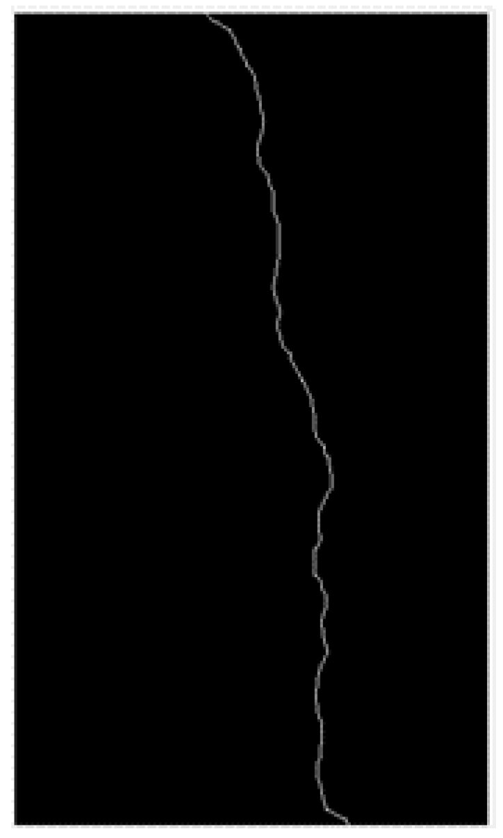
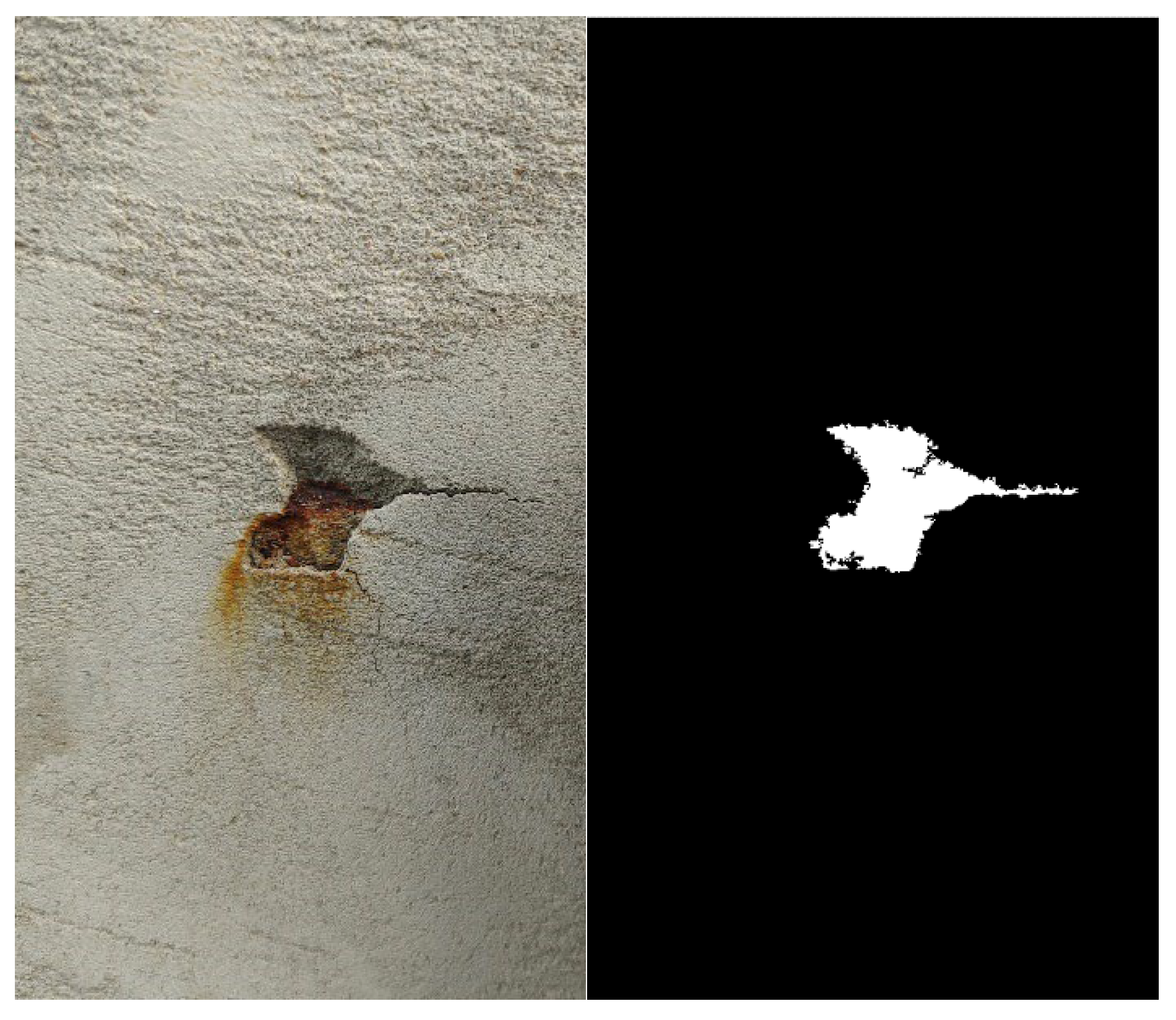
• In the process of image collection, the image information collected is too complex due to the environment, noise, equipment and other problems, which increases the difficulty of damage information extraction, so the image needs to be processed. The process is as follows:
  • The image is grayed by weighted average method.
  • The method of gray adjustment is used to enhance the image.
  • The image is denoised by linear filter.
  • The Otsu binarization method is used to segment the image.
  • The final binary image is obtained by removing the interference of small area image and morphological calculation.
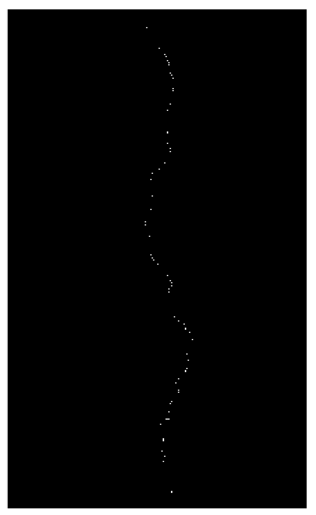
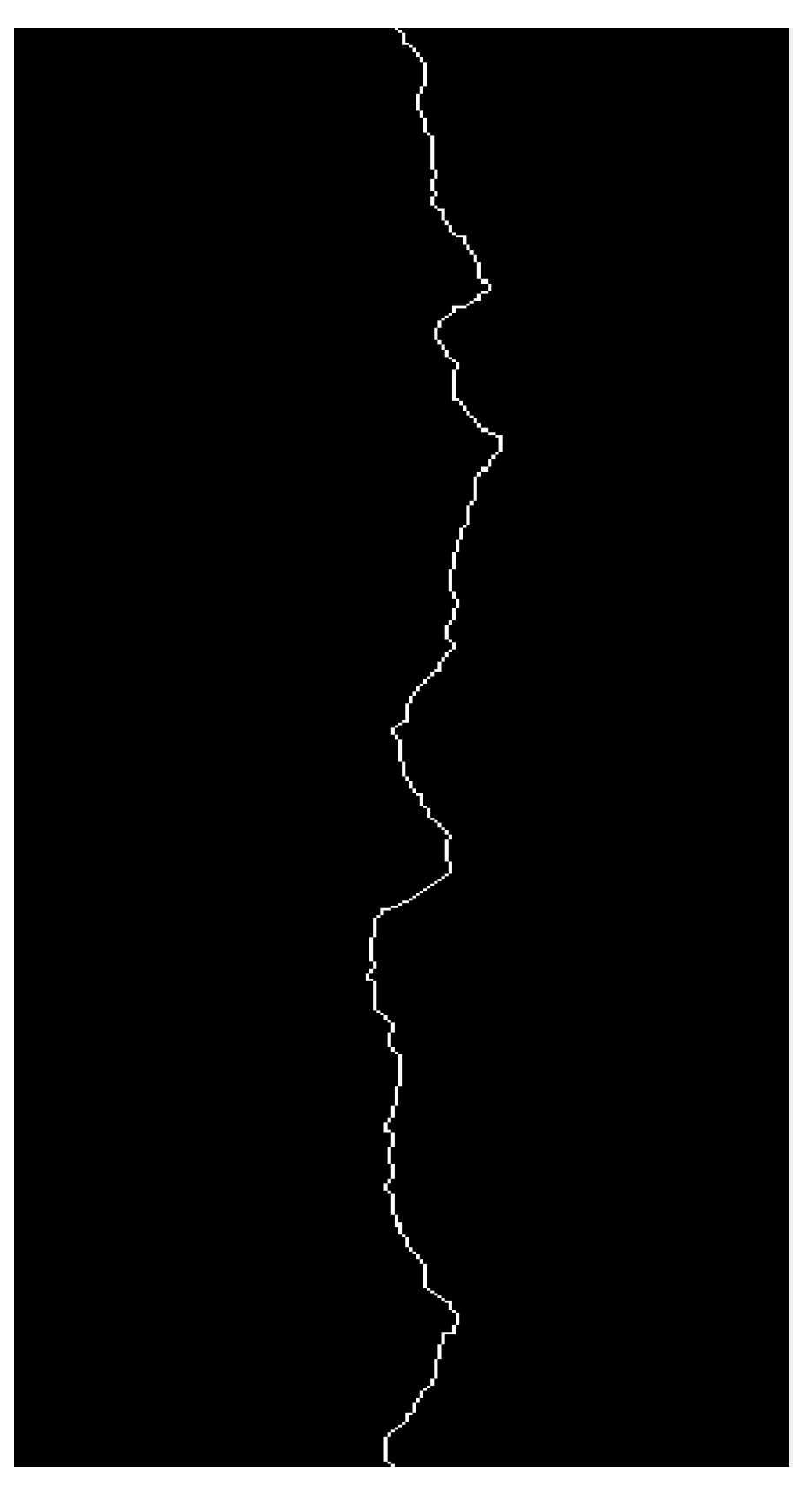
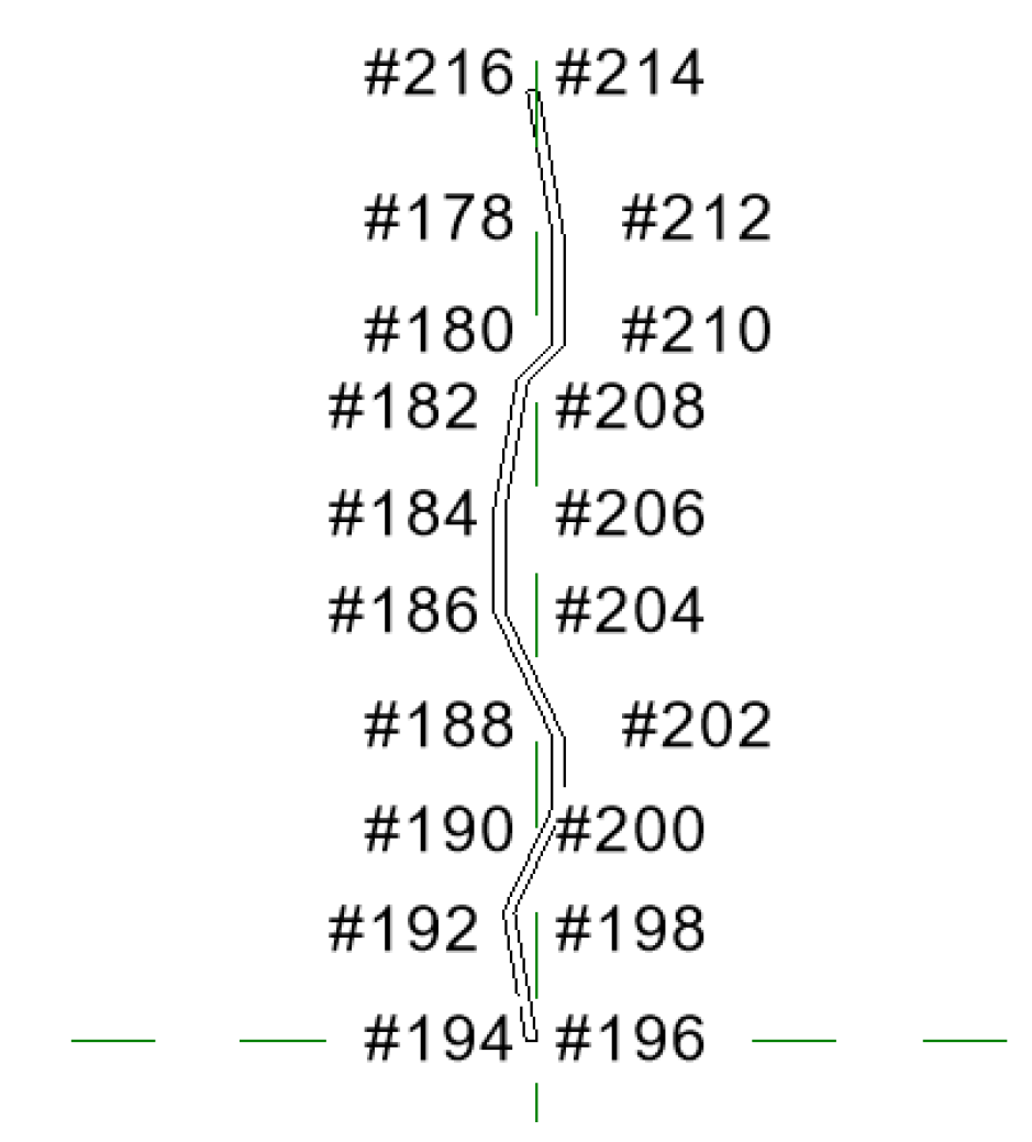
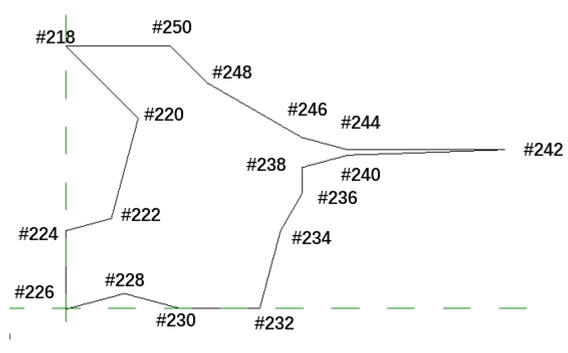
• The relevant information can be extracted after processing the damage image. The skeleton method extracts the crack into the crack skeleton connected by a single pixel. The pixel point statistics method counts the pixel points of crack length, width and damage area. The actual length, width and area are obtained by converting with the actual size.
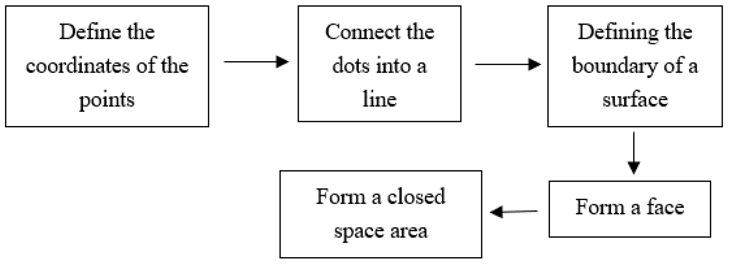
• The damage model is established by the method of boundary representation. The bridge model and the damage are represented as many curved surfaces connected to form a closed space area through the points, lines, planes and the mutual relations to form the bridge model with damage and realize the visualization of the bridge damage.

References

1. Jin, M.; Huang, Z.; Han, Z.; Han, F. Research on Bridge Crack Width Detection Based on Matlab Image Processing Method. J. China Foreign Highw. 2017, 37, 120–123. [Google Scholar] [CrossRef]
2. Zuo, D. Research on Bridge Crack Measurement Method Based on Digital Image Processing; Shijiazhuang Tiedao University: Shijiazhuang, China, 2017. [Google Scholar]
3. Wang, Q.; Dong, X.; Shen, Z.; Xiong, G.; Yan, J.; Niu, L. An Image-based Automatic Calculation Algorithm for Bridge Crack Size. In Proceedings of the 2019 Chinese Automation Congress (CAC), Hangzhou, China, 22–24 November 2019. [Google Scholar]
4. Wang, L. Research on Digital Image Processing Algorithms for Crack Recognition of Concrete Dams; Dalian University of Technology: Dalian, China, 2019. [Google Scholar] [CrossRef]
5. Xiao, Z.; Han, H.; Xu, Y. Research on Key Technology of Pavement Crack Recognition Based on Digital Image Processing. J. Jilin Norm. Univ. 2022, 43, 116–120. [Google Scholar] [CrossRef]
6. Cevallos-Torres, L.J.; Minda Gilces, D.; Guijarro-Rodriguez, A.; Barriga-Diaz, R.; Leyva-Vazquez, M.; Botto-Tobar, M. An Approach to the Detection of Post-Seismic Structural Damage Based on Image Segmentation Methods; Springer: Cham, Switzerland, 2019. [Google Scholar]
7. Tan, X.; Xu, G.; Song, J.; Zhang, J.; Zhou, R.; Yu, T. Recognition of Concrete Surface Cracks Based on Digital Image Processing Technology. Low Temp. Archit. Technol. 2020, 42, 11–13. [Google Scholar] [CrossRef]
8. Shao, Y.; Wang, X.; Ren, X.; Yang, C.; Liu, B.; Shan, Y. Semi-automatic Detection Method of Bridge Crack Based on Computer Vision. J. Guizhou Univ. Financ. Econ. 2019, 15, 176–179. [Google Scholar]
9. Shi, L.; Yu, Z. Research on On-line Detection Method of Oil Seal Defect Based on Image Processing. J. Chang. Univ. Sci. Technol. 2021, 44, 48–54. [Google Scholar]
10. Shen, G. Road crack detection based on video image processing. In Proceedings of the 2016 3rd International Conference on Systems and Informatics (ICSAI), Shanghai, China, 19–21 November 2016; pp. 912–917. [Google Scholar]
11. Yang, B. Research on Visualization of Bridge Structure Health Monitoring Information Based on BIM; Chongqing Jiaotong University: Chongqing, China, 2018. [Google Scholar]
12. Xu, S.; Wang, J.; Wang, X.; Wu, P.; Shou, W.; Liu, C. A Parameter-Driven Method for Modeling Bridge Defects through IFC. J. Comput. Civ. Eng. 2022. [Google Scholar] [CrossRef]
13. Cao, B. Research on Integration and Visualization of Bridge Construction Monitoring Data Based on IFC; Nanjing Forestry University: Nanjing, China, 2020. [Google Scholar] [CrossRef]
14. Shi, P. Research on the IFC-Based Component Library; Shanghai Jiao Tong University: Shanghai, China, 2014. [Google Scholar]
15. Chu, H. Research on Visual Expression of Bridge Diseases. Master’s Thesis, Huazhong University of Science and Technology, Wuhan, China, 2020. [Google Scholar] [CrossRef]
16. Bao, L.; An, P.; Wang, P.; Liang, W.; Yu, L. Research on Visualization of Bridge Safety Information Based on IFC. J. Shenyang Jianzhu Univ. 2022, 38, 682–689. [Google Scholar]
17. Wu, Y. Concrete crack information analysis based on IFC standard. J. Guizhou Univ. Financ. Econ. 2017, 13, 157–158. [Google Scholar]
18. Ma, J.; Chu, H.; Kong, L.; Guo, X.; Bai, Y. IFC-based Visual Expression of Bridge Damage Information. J. Civ. Eng. Manag. 2020, 37, 66–72. [Google Scholar]
19. Hüthwohl, P.; Brilakis, I.; Borrmann, A.; Sacks, R. Integrating RC Bridge Defect Information into BIM Models. J. Comput. Civ. Eng. 2018, 32. [Google Scholar] [CrossRef]
20. Isailović, D.; Stojanovic, V.; Trapp, M.; Richter, R.; Hajdin, R.; Döllner, J. Bridge damage: Detection, IFC-based semantic enrichment and visualization. Autom. Constr. 2020, 112, 103088. [Google Scholar] [CrossRef]
21. Lim, J.S. Two-Dimensional Signal and Image Processing; Equations 9.44, 9.45, and 9.46; Prentice Hall: Englewood Cliffs, NJ, USA, 1990; p. 548. [Google Scholar]
Figure 1. The original images of the damages. (a) Original image of crack; (b) Original image of concrete cavity with exposed bars.
Sustainability 15 08769 g001
Figure 2. The damaged image after processing. (a) Image of Crack after processing; (b) Image of exposed reinforcement of concrete cavity after processing.
Sustainability 15 08769 g002
Figure 3. The skeleton of the crack.
Sustainability 15 08769 g003
Figure 4. Part of the IFC code.
Sustainability 15 08769 g004
Figure 5. Flowchart of modeling using the IFC standard.
Sustainability 15 08769 g005
Figure 6. Concrete block with cracks.
Sustainability 15 08769 g006
Figure 7. Bridge Elevation.
Sustainability 15 08769 g007
Figure 8. Tower Elevation.
Sustainability 15 08769 g008
Figure 9. Sectional view of the main beam.
Sustainability 15 08769 g009
Figure 10. Processing of crack image.
Sustainability 15 08769 g010
Figure 11. Skeleton of the crack.
Sustainability 15 08769 g011
Figure 12. Enlarged local crack skeleton.
Sustainability 15 08769 g012
Figure 13. Image processing of concrete defects.
Sustainability 15 08769 g013
Figure 14. Model of the main girder.
Sustainability 15 08769 g014
Figure 15. Model of cable-stayed bridge.
Sustainability 15 08769 g015
Figure 16. Feature points of main beam.
Sustainability 15 08769 g016
Figure 17. Characteristic points of cracks.
Sustainability 15 08769 g017
Figure 18. Characteristic points of concrete defects.
Sustainability 15 08769 g018
Figure 19. Models of cracks and concrete defects.
Sustainability 15 08769 g019
Disclaimer/Publisher’s Note: The statements, opinions and data contained in all publications are solely those of the individual author(s) and contributor(s) and not of MDPI and/or the editor(s). MDPI and/or the editor(s) disclaim responsibility for any injury to people or property resulting from any ideas, methods, instructions or products referred to in the content.